Machine Learning-Based Microclimate Model for Indoor Air Temperature and Relative Humidity Prediction in a Swine Building - MDPI

Page created by Alfred French
 
CONTINUE READING
Machine Learning-Based Microclimate Model for Indoor Air Temperature and Relative Humidity Prediction in a Swine Building - MDPI
animals
Article
Machine Learning-Based Microclimate Model for Indoor Air
Temperature and Relative Humidity Prediction in a Swine Building
Elanchezhian Arulmozhi                     , Jayanta Kumar Basak, Thavisack Sihalath, Jaesung Park, Hyeon Tae Kim
and Byeong Eun Moon *

                                            Department of Bio-Systems Engineering, Institute of Smart Farm, Gyeongsang National University,
                                            Jinju 52828, Korea; mohanachezhian@yahoo.com (E.A.); basak.jkb@gmail.com (J.K.B.); max7set@gmail.com (T.S.);
                                            jaesung.park@gnu.ac.kr (J.P.); bioani@gnu.ac.kr (H.T.K.)
                                            * Correspondence: be25moon@naver.com; Tel.: +82-10-4548-9004

                                            Simple Summary: Indoor air temperature (IAT) and indoor relative humidity (IRH) are the promi-
                                            nent microclimatic variables. Among other livestock animals, pigs are more sensitive to environmen-
                                            tal equilibrium; a lack of favorable environment in barns affects the productivity parameters such as
                                            voluntary feed intake, feed conversion, heat stress, etc. Machine learning (ML) based prediction mod-
                                            els are utilized for solving various nonlinear problems in the current decade. Meanwhile, multiple
                                            linear regression (MLR), multilayered perceptron (MLP), random forest regression (RFR), decision
                                            tree regression (DTR), and support vector regression (SVR) models were utilized for the prediction.
                                            Typically, most of the available IAT and IRH models are limited to feed the animal biological data as
                                            the input. Since the biological factors of the internal animals are challenging to acquire, this study
                                            used accessible factors such as external environmental data to simulate the models. Three different
                                            input datasets named S1 (weather station parameters), S2 (weather station parameters and indoor
                                  attributes), and S3 (Highly correlated values) were used to assess the models. From the results, RFR
         
                                            models performed better results in both IAT (R2 = 0.9913; RMSE = 0.476; MAE = 0.3535) and IRH
Citation: Arulmozhi, E.; Basak, J.K.;       (R2 = 0.9594; RMSE = 2.429; MAE = 1.47) prediction with S3 input datasets. In addition, it has been
Sihalath, T.; Park, J.; Kim, H.T.; Moon,
                                            proven that selecting the right features from the given input data builds supportive conditions under
B.E. Machine Learning-Based
                                            which the expected results are available.
Microclimate Model for Indoor Air
Temperature and Relative Humidity
                                            Abstract: Indoor air temperature (IAT) and indoor relative humidity (IRH) are the prominent
Prediction in a Swine Building.
                                            microclimatic variables; still, potential contributors that influence the homeostasis of livestock animals
Animals 2021, 11, 222. https://
doi.org/10.3390/ani11010222
                                            reared in closed barns. Further, predicting IAT and IRH encourages farmers to think ahead actively
                                            and to prepare the optimum solutions. Therefore, the primary objective of the current literature is to
Received: 28 December 2020                  build and investigate extensive performance analysis between popular ML models in practice used
Accepted: 13 January 2021                   for IAT and IRH predictions. Meanwhile, multiple linear regression (MLR), multilayered perceptron
Published: 18 January 2021                  (MLP), random forest regression (RFR), decision tree regression (DTR), and support vector regression
                                            (SVR) models were utilized for the prediction. This study used accessible factors such as external
Publisher’s Note: MDPI stays neutral        environmental data to simulate the models. In addition, three different input datasets named S1, S2,
with regard to jurisdictional claims in     and S3 were used to assess the models. From the results, RFR models performed better results in both
published maps and institutional affil-     IAT (R2 = 0.9913; RMSE = 0.476; MAE = 0.3535) and IRH (R2 = 0.9594; RMSE = 2.429; MAE = 1.47)
iations.
                                            prediction among other models particularly with S3 input datasets. In addition, it has been proven
                                            that selecting the right features from the given input data builds supportive conditions under which
                                            the expected results are available. Overall, the current study demonstrates a better model among
                                            other models to predict IAT and IRH of a naturally ventilated swine building containing animals
Copyright: © 2021 by the authors.           with fewer input attributes.
Licensee MDPI, Basel, Switzerland.
This article is an open access article
                                            Keywords: indoor air temperature; indoor relative humidity; swine building microclimate; ML
distributed under the terms and
                                            models; smart farming
conditions of the Creative Commons
Attribution (CC BY) license (https://
creativecommons.org/licenses/by/
4.0/).

Animals 2021, 11, 222. https://doi.org/10.3390/ani11010222                                                    https://www.mdpi.com/journal/animals
Machine Learning-Based Microclimate Model for Indoor Air Temperature and Relative Humidity Prediction in a Swine Building - MDPI
Animals 2021, 11, 222                                                                                             2 of 24

                        1. Introduction
                        1.1. Research Significance
                             Climate change has intensified the impacts against agriculture production over the
                        past few decades that makes bewilderment on the livelihoods of farmers and consumers. In
                        the current scenario, producing high quality agricultural products using traditional farming
                        methodologies is becoming arduous for the farmers. In 2030, the world would have to feed
                        more than 8 billion people, whereas maintaining sustainable farming methodologies is an
                        enormous challenge for food security [1]. Economic experts estimate the demand for milk
                        and meat by 2050 could increase by 70 to 80% over current market demand [2]. However,
                        extreme weather conditions directly affect the livestock sector in several ways, such as
                        productivity losses, biological changes, and welfare issues [2]. There is a demand to adopt
                        modern farming methods such as smart livestock farming (SLF), which are alternatives
                        to conventional farming methods to address these challenges. SLF can provide optimal
                        control strategy with the help of inexpensive and improved sensors availability, actuators
                        and microprocessors, high performance computational software, cloud-based ICT systems,
                        and big data analytics. The significance of well-managed animal welfare is not narrow to
                        ethical aspects; it is vital to realize an effective action of provoking animal commodities.
                             Maintaining a favorable environment in livestock building would assist in producing
                        qualitative and healthier outcomes. The preeminent intention of adopting the SLF is
                        to regulate the indoor microclimatic parameters like temperature and humidity at the
                        optimum level [3]. The characteristics of indoor microclimate immensely influence the
                        livestock production aspects such as animal health and welfare. The pigs are more sensitive
                        to indoor climatic parameters than all other livestock, so that a constant temperature and
                        humidity are the essential factors for their routine activities. In general, 16–25 ◦ C of indoor
                        temperature and 60–80% of indoor humidity are considered the optimal environment
                        for pigs; such an environment is called a thermo-neutral zone (TNZ) [4,5]. The TNZ
                        provides the welfare of animals, resulting in enhancing the voluntary feed intake and
                        minimizing thermal and other environmental stress [6]. Maintaining proper temperature
                        and relative humidity within the pig’s TNZ is the primary function of a microclimate
                        controlling system [7]. Modelling the microclimate of livestock building by using outdoor
                        parameters helps to regularize the indoor environment condition; moreover, it may guide
                        the preparation of precautions from extreme outdoor conditions.
                             The indoor microclimate dynamics are majorly affected by the outdoor disturbance
                        generated from either seasonal or daily meteorological changes being outdoor temperature
                        variations, humidity changes, rainfall fluctuation, etc. Advanced microclimate models
                        are vital to make microclimate controllers as smart, which may also act as supplementary
                        to boost the controllers’ strategy. Heretofore researchers developed several models as
                        dynamic, steady-state models, heat balance equations, computational fluid dynamics to
                        predict indoor air temperature (IAT), and indoor relative humidity (IRH). Most of the
                        previous models were developed by using the theoretical relationship between heat and
                        mass transfer functions, energy-oriented facets, and indoor fluid dynamics [3,8–10]. Such
                        mechanisms require complex information such as airflow dynamics, animal information,
                        and fan specifications to derive the equations. Nevertheless, such kinds of models are
                        limited to quality, quantity, missing values of data while predicting the naturally ventilated
                        building’s IAT and IRH. Collecting attributes of those variables mentioned earlier are
                        convoluted; thus, adopting advanced modeling techniques like artificial intelligence (AI) is
                        key to simulate the microclimate in easier way.
                             Machine learning (ML) is a subdivision of AI, has reinterpreted the world in diverse
                        forecasting fields for the past two decades. The rapid advancement of graphics rendering
                        and computer synchronization combined is the reason for the excessive growth of ML
                        popularity than other prediction methods [11]. The ML models are capable of adaptive
                        learning from the data, and it can improve themselves from subsequent training, trends,
                        and pattern identification. Such inherent characteristics have driven them to handle
                        complex investigations effectively. Applying such technologies could analyze the large
Machine Learning-Based Microclimate Model for Indoor Air Temperature and Relative Humidity Prediction in a Swine Building - MDPI
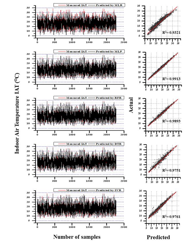
Animals 2021, 11, 222                                                                                            3 of 24

                        data sets more effectively with relative ease than physical or statistical models. Especially
                        for determining linear and nonlinear variables that follow time-series such as indoor
                        microclimate modelling field, the ML-based models have proven it outperformed the
                        statistical models [10]. Several training algorithms are available for the ML framework,
                        including linear regression (LR), decision trees regression (DTR), random forest regression
                        (RFR), support vector regression (SVR), etc., have been developed to handle the regression
                        and classification problems. Previous studies utilized artificial neural network (ANN) and
                        ML models to predict the variables related to animal studies. For instance, ref. [10] utilized
                        an ANN model to predict a swine building’s temperature and relative humidity, whereas
                        the growth performance of swine was analyzed with decision trees and support vector
                        machines by a previous study [12]. Likewise, ref. [13] predicted the skin temperature of
                        pigs based on the indoor parameters using an MLP. A previous study [14] employed MLP
                        and classification and regression trees (CART) algorithms to predict piglets’ core, skin, and
                        hair-coat temperatures.

                        1.2. Research Objectives
                              Through achieved significant certainty, ML models have been utilized to work out dis-
                        putes such as prediction, classification, clustering, etc. Nevertheless, there is a knowledge
                        gap in utilizing advanced modelling techniques to simulate the microclimate of a livestock
                        building [15]. The current study tries to evaluate the performance of usual ML models
                        while simulating the IAT and IRH of a swine building.
                              Research on the depth and breadth of the applications and the state of the art of
                        ML-based predictions of IAT and IRH of pig barn containing animals are scarce. Several
                        models have been successfully developed and implemented to predict microclimate of
                        other smart farm buildings like a greenhouse and plant factory. Like the other smart farm,
                        ML models could be adopted in order to regulate the microclimate of pig buildings after
                        optimization and calibration. Previous researchers mostly develop a single model and
                        simulate the attributes and validation; therefore, the model’s robustness becomes a dispute.
                        For instance, Ref. [10] employed a multilayered perceptron with a backpropagation model
                        to predict the IAT and IRH of a swine building, and evaluate the model without comparison
                        with other models. In contrast, refs. [16,17] simulates the indoor microclimate using the
                        autoregressive integrated moving average (ARIMA) model. A comprehensive comparison
                        and analysis between the other popular model performances lack such literature; those
                        studies build a model and validate it quickly. Therefore, the leading intention of the current
                        study is to build and investigate extensive performance analysis between popular ML
                        models in practice used for IAT and IRH predictions.
                              Typically, indoor climatic parameters of any animal buildings are dependent variables
                        that are subject to significant change by the external environmental parameters. Unlike
                        mechanically ventilated buildings, naturally ventilated swine buildings indoor IAT and
                        IRH aerodynamics eminently vulnerable to outdoor climate and biological factors of the
                        animals present [18]. The outdoor climate data is accessible and ubiquitous, whereas
                        collecting biological data involves skin temperature, behavioral changes, health aspects,
                        etc. It is not limited to predicament data acquisition; it also affects the physical equilibrium
                        and homeostasis of the animals while collecting data [19]. Considering the above factors,
                        the current research used accessible factors such as external environmental data without
                        considering the biological factor of the animals to simulate the models.
                              Determination of input data is the bottom line of any modelling criteria yet crucial
                        consideration in diagnosing the exquisite functional form of ML models. Choosing the right
                        input variables involves improving the accuracy of the algorithm; also, it dominates the
                        calculation speed, training time, training complexity, comprehensibility, and computational
                        effort of the simulation [20–22]. The present study analyzes the performance of the models
                        with feature-selected datasets and available datasets; it also suggests the optimal input
                        selection to feed the models from the available datasets.
Machine Learning-Based Microclimate Model for Indoor Air Temperature and Relative Humidity Prediction in a Swine Building - MDPI
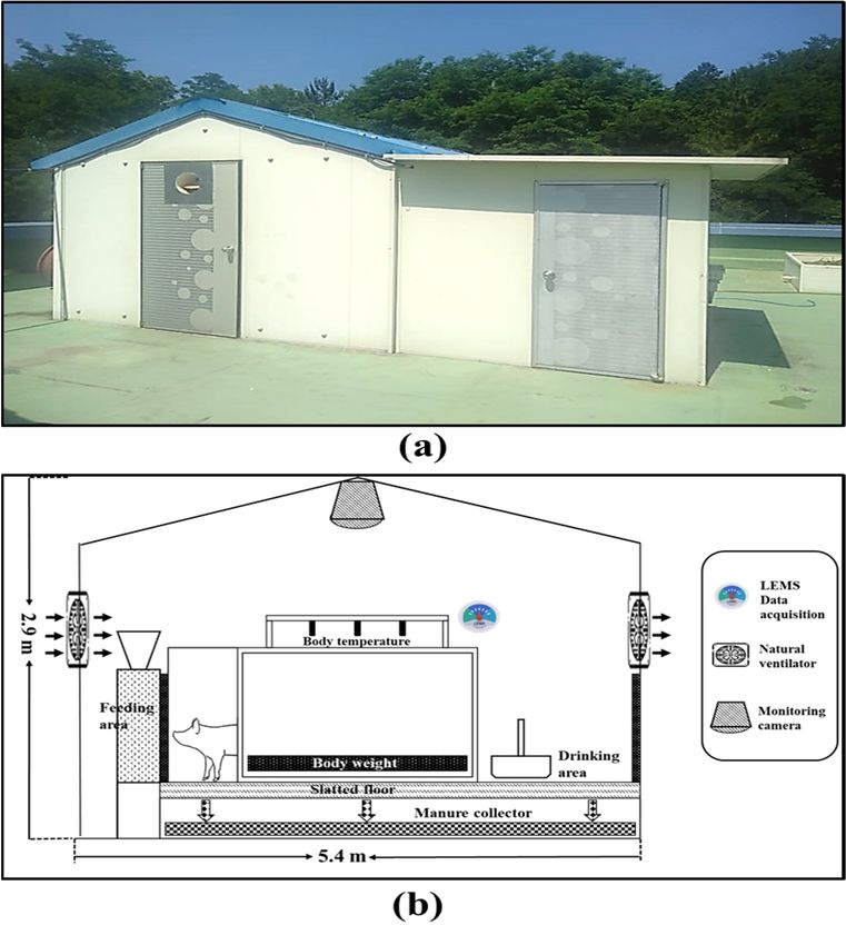
Animals 2021, 11, x                                                                                                            4 of 25

Animals 2021, 11, 222                                                                                                          4 of 24
                         the models with feature-selected datasets and available datasets; it also suggests the opti-
                         mal input selection to feed the models from the available datasets.

                        2.2.Materials
                             Materialsand
                                       andMethods
                                            Methods
                        2.1.
                          2.1. Arrangement ofSwine
                             Arrangement  of  SwineBuilding
                                                    Building
                              The
                                Thecurrent
                                     currentstudy
                                               studywaswasconducted
                                                            conductedatata amodel
                                                                               modelswineswinebuilding
                                                                                                buildinglocated
                                                                                                           locatedininGyeongsang
                                                                                                                        Gyeongsang
                        National    University,    Jinju-Si,  the  Republic   of   Korea,    with  2.9
                          National University, Jinju-Si, the Republic of Korea, with 2.9 m width × 5.4 m  width    ×m5.4length
                                                                                                                          m length
                                                                                                                                 × 0.05
                        ×m0.05   m  thick roofs  as  shown   in  Figure 1. The    GPS   coordinates   for the site was  35 ◦ 090 6.26”
                             thick roofs as shown in Figure 1. The GPS coordinates for the site was 35°09′6.26″                      N,
                        N,  128◦ 050 43.838”
                          128°05′43.838″        E [23].
                                            E [23].  TheThe
                                                         heatheat    conduction
                                                                conduction           is diminished
                                                                             is diminished      by overby 40%
                                                                                                          overwhile
                                                                                                                 40% while     utiliz-
                                                                                                                       utilizing   slat-
                        ing
                          tedslatted
                               floors floors  compared
                                       compared      to thetoconcrete
                                                               the concrete
                                                                        floorsfloors
                                                                                 in a in   a naturally
                                                                                        naturally       ventilated
                                                                                                    ventilated  pig pig
                                                                                                                     barnbarn
                                                                                                                            [24].[24].
                                                                                                                                   The
                        The   model   swine   building   used   polypropylene      copolymer      slatted floors
                          model swine building used polypropylene copolymer slatted floors to decrease heat trans-to decrease    heat
                        transmission,
                          mission, and and     the total
                                          the total  areaarea   ofbarn
                                                           of the  the barn  was 13.26
                                                                        was 13.26           m2 (1.32
                                                                                      m2 (1.32         m2 /pig).
                                                                                                m2/pig).          Ten crossbreeds
                                                                                                          Ten crossbreeds     (Amer-
                        (American     Yorkshire    ×  Duroc)    pigs  with an   average     body  weight
                          ican Yorkshire × Duroc) pigs with an average body weight of 86.4–142.4 kg were   of 86.4–142.4    kg grown
                                                                                                                                were
                        grown    in the  model   swine   building   throughout      the   experimental   time.  The
                          in the model swine building throughout the experimental time. The trial building incor-    trial building
                        incorporates     an automatic
                          porates an automatic            infrared
                                                    infrared         sensor-based
                                                               sensor-based    feederfeeder    (robust
                                                                                         (robust        military
                                                                                                 military          automatic
                                                                                                           automatic             feed
                                                                                                                        feed system,
                        system,   South   Korea)   integrated    with  the body    weight    and  body   temperature
                          South Korea) integrated with the body weight and body temperature estimation scales.           estimation
                        scales. The pigs were offered nutritionally balanced dry feed to meet apparent digestible
                          The pigs were offered nutritionally balanced dry feed to meet apparent digestible energy
                        energy (DE) 3500 kcal/kg twice a day (09:00 h and 17:00 h). The pigs were provided 1.5–3.2
                          (DE) 3500 kcal/kg twice a day (09:00 h and 17:00 h). The pigs were provided 1.5–3.2
                        kg/day/pig of dry feed, as suggested by the Institutional Animal Care and Use Committee
                          kg/day/pig of dry feed, as suggested by the Institutional Animal Care and Use Committee
                        (IACUC) of Gyeongsang national university during the overall experimental time.
                          (IACUC) of Gyeongsang national university during the overall experimental time.

                        Figure 1. (a) Outdoor view of the model swine building which was used for current experiment; (b)
                         Figure 1. (a) Outdoor view of the model swine building which was used for current experiment;
                        sensor placement
                         (b) sensor       and indoor
                                     placement       schematic
                                               and indoor       of model
                                                           schematic     swineswine
                                                                     of model  building.
                                                                                    building.
                        2.2. Sensor Data
                             A research-grade weather station (model: MetPRO, Producer: Campbell Scientific,
                        Logan, UT, USA) was installed at 26 m away from the model swine building to collect the
                        outdoor climatic variable, used as a predictor/independent variables. A digital air tem-
                        perature and humidity sensor (CS215-L), a wind sentry set with an anemometer (03002-L),
Machine Learning-Based Microclimate Model for Indoor Air Temperature and Relative Humidity Prediction in a Swine Building - MDPI
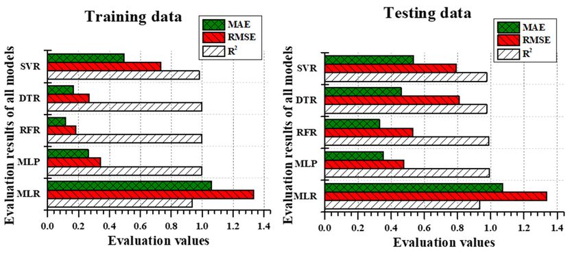
Animals 2021, 11, 222                                                                                                             5 of 24

                           rain gage with a 6-inch orifice (TE525-L), pyranometer (CS300-L), barometric pressure
                           Sensor (CS100), and reflectometer (CS655), such customized sensors were comprised to the
                           weather station for the data reception. A data logger (model: CR1000X), which is capable
                           of storing the data from the sensors and parallel transportation of data to the computer,
                           was annexed to the weather station. Indoor microclimatic parameters were recorded by
                           utilizing a livestock environment management system (LEMS, AgriRoboTech Co., Ltd.,
                           Gyeonggi, South Korea), which is capable of acquiring data from inside of pig barn and
                           store the accumulated data. The collected data considered as the response variable for the
                           current study. However, the weather station and LEMS data were stored in the database
     Animals 2021, 11, x   management system for analysis purposes. The complete details of the sensor, 6 of 25 sensor
                           placement, and equipped devices are disclosed in Figures 1b and 2 in a detailed manner.

                            Figure 2. Devices used for data acquisition of indoor (LEMS) and outdoor (Campbell scientific
                           Figure 2. Devices used for data acquisition of indoor (LEMS) and outdoor (Campbell scientific
                            weather station) including sensor extensions; data transmission process during LEMS and
                           weather
                            CR1000Xstation)   including
                                     data storage  to the sensor
                                                          primaryextensions;
                                                                  database. data transmission process during LEMS and CR1000X
                           data storage to the primary database.
                            2.3. Approach
                             2.3.1.For this study,
                                    Multiple       each
                                              Linear     computerized
                                                     Regression    Model sensor data was stored at 10-min intervals according
                           to the experimental design from 17 September to 5 December 2019. During the experimental
                                   Multiple linear regression models (MLR) are commonly used empirical models to
                           time,
                             solve pigs  were grown
                                     nonlinear          in the
                                                problems.    Thesemodel   swine
                                                                     models   are building.
                                                                                    also popular Since  the final
                                                                                                    among          goal of
                                                                                                             the fields    thisasresearch
                                                                                                                         such
                           isweather
                               to optimize
                                       prediction, electricity load, energy consumption, heat transfer, business forecast,Overall,
                                              the actuators,    the  model   pig   barn   was    considered    as a  prototype.
                           2etc.
                              response
                                 [25–28].variables
                                           Generally,and  10 predictor
                                                      regression    models variables
                                                                            examine data      were used
                                                                                       the relative       for the
                                                                                                     influence      analysis.
                                                                                                                of the        The details
                                                                                                                       independ-
                           ofent
                               collected   independent     and   dependent     variables    with   unit, mean,    minimum,
                                 variables or predictor variables on the dependent variables or response variables. MLR       maximum,
                           and   standard
                             models          deviation
                                      are popular  among (SD)
                                                            the are  explained
                                                                 forecast because inofTable
                                                                                        their 1. The indoorstructures,
                                                                                              non-complex      microclimate     may have
                                                                                                                         calcula-
                             tion interpretability,
                           affected                 and the
                                       by the biological      ability
                                                           factors  oftothe
                                                                          identify
                                                                            animals outliers
                                                                                        such oras anomalies   in given predictor
                                                                                                  body temperature,      water drinking,
                             variables.
                           feed   intake,Anetc.
                                             MLR  model
                                                Since thecan   be expressed
                                                           primary    objectiveby the  following
                                                                                   of the  study isequation  [25–28],
                                                                                                      modeling    the indoor parameter
                           by considering the outdoor parameters,             the  current
                                                               Y = a + a X + a X +…+ a X + Ɛ  research   averts  biological  factors.
                                                                                                                               (1)
                                                                   0   1   1   2   2      i   i

                            where Y is the response (output) variable; X is the predictor (independent) variable (from
                            X1 to Xi); a is the regression coefficient to predict Y (from a1 to ai); a0 is the intercept/con-
                            stant of the model; and the Ɛ is the noise or random error of the model.

                            2.3.2. Decision Tree Regression Model
                                 Unlike other ML models that are considered as a black-box model while operation,
Machine Learning-Based Microclimate Model for Indoor Air Temperature and Relative Humidity Prediction in a Swine Building - MDPI
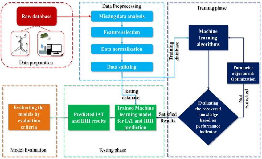
Animals 2021, 11, 222                                                                                                 6 of 24

                        Table 1. Descriptive statistics and profile information of the outdoor/predictor data collected
                        from weather station (Campbell scientific weather station) and indoor/response data collected
                        from LEMS sensors.

                         S. No    Attribute Elements/Predictors (Unit)           Mean ± SD          SE      Min      Max
                            1     WD        Wind direction  (◦ (Azimuth))        205.0 ± 67.43     0.632     29.4    337.2
                            2      WS            Wind speed (m/s)                0.644 ± 0.379     0.003     0.11     4.55
                            3     OAT      Outdoor air temperature (◦ C)         12.858 ± 6.729    0.063    −2.7       31
                            4     ORH      Outdoor relative humidity (%)        72.746 ± 22.082    0.207    13.78     96.9
                            5      AP        Outdoor air pressure (Pa)         1013.916 ± 5.495    0.051     976     1024
                            6     RFA         Rain fall amount (inch)            0.0057 ± 0.059    0.0005      0      1.71
                            7     SLR        Solar irradiance (Wm-2)          124.722 ± 199.280    1.869      0       889
                            8     SMC        Soil moisture content (%)          17.325 ± 1.722     0.016    13.88    29.62
                            9      ST      Outdoor soil temperature (◦ C)        13.851 ± 6.229    0.058    2.622    30.26
                           10     CNR          Net radiation (Wm-2)           31.037 ± 149.867     1.406    −161.8   645.1
                         S. No    Attribute Elements/Response (Unit)            Mean ± SD           SE      Min      Max
                           1       IAT       Indoor air temperature (◦ C)       18.294 ± 5.22      0.048    6.7      34.2
                           2       IRH      Indoor relative humidity (%)       70.122 ± 12.179     0.114    25.5     92.3

                        2.3. Approach
                        2.3.1. Multiple Linear Regression Model
                             Multiple linear regression models (MLR) are commonly used empirical models to
                        solve nonlinear problems. These models are also popular among the fields such as weather
                        prediction, electricity load, energy consumption, heat transfer, business forecast, etc. [25–28].
                        Generally, regression models examine the relative influence of the independent variables
                        or predictor variables on the dependent variables or response variables. MLR models
                        are popular among the forecast because of their non-complex structures, calculation inter-
                        pretability, and the ability to identify outliers or anomalies in given predictor variables. An
                        MLR model can be expressed by the following equation [25–28],

                                                      Y = a0 +a1 X1 +a2 X2 + . . . + ai Xi + ε                           (1)

                        where Y is the response (output) variable; X is the predictor (independent) variable (from X1
                        to Xi ); a is the regression coefficient to predict Y (from a1 to ai ); a0 is the intercept/constant
                        of the model; and the ε is the noise or random error of the model.

                        2.3.2. Decision Tree Regression Model
                              Unlike other ML models that are considered as a black-box model while opera-
                        tion, decision tree regression (DTR) models are own opposite characteristics among the
                        other models. Compared to the other supervised algorithms, DTR is popular for the
                        self-explanatory/rule-based by nature; data interpretability for a response subject to the
                        predictor variables could formulate visually [11]. DTR models were initially developed to
                        solve the classification problem and manipulated to solve the classification and regression
                        problem (CAR). The schematic diagram of the DTR model is shown in Figure 3a, where
                        each node represents features, each branch of the tree represents a rule/decision, and
                        each leaf of the tree represents regression values. The DTR models predict the output by
                        calculating the probability of an outcome based on the feature influence. DTR uses the
                        entropy function and information gain as the relevant metrics of each attribute to determine
                        the desired output. Entropy/information entropy is used to measure the homogeneity of
                        an arbitrary collection of samples. The information gain is applied to calculate the amount
                        of an attribute, which contributes to estimating the classes. The entropy and information
                        gain can be expressed by the following Equations (2) and (3) [11,29,30],

                                                                     CT
                                                            H =−     ∑ pTi · log2 (pTi )                                 (2)
                                                                    c=1
Machine Learning-Based Microclimate Model for Indoor Air Temperature and Relative Humidity Prediction in a Swine Building - MDPI
output. Entropy/information entropy is used to measure the homogeneity of an arbitrary
                                collection of samples. The information gain is applied to calculate the amount of an attrib-
                                ute, which contributes to estimating the classes. The entropy and information gain can be
                                expressed by the following Equations (2) and (3) [11,29,30],
Animals 2021, 11, 222                                                           CT                                               7 of 24
                                                                        H =−         pTi .log2 pTi                                  (2)
                                                                               c=1

                                                                                                     nn
                                                                                                     ||T
                                                                                                      Tii||
                                                         Information Gain((X,T)
                                                          InformationGain  X, T)= H(T) − ∑
                                                                                = H(T)                     ·.HH(T(T
                                                                                                                  i )i )             (3)
                                                                                                                                    (3)
                                                                                                 i=1 ||T|
                                                                                                       T|
                                                                                                     i=1
                                 whereppTiTiisisthe
                                where            theproportion
                                                     proportionofofdata
                                                                    datapoints;
                                                                          points;CCTTisisthe
                                                                                          thetotal
                                                                                              totalnumber
                                                                                                   numberof  of classes;
                                                                                                                classes; TTiiisisthe
                                                                                                                                  theone
                                                                                                                                     one
                                 sample  among      all the n subsets in which the  total   amount  of training  data T
                                sample among all the n subsets in which the total amount of training data T was divided   was    divided
                                 dueto
                                due  toan
                                        anattribute
                                             attributeX. X.

                 Importantparameters
      Figure3.3.Important
     Figure                  parameters  and
                                       and    operational
                                            operational   blue
                                                        blue    print
                                                             print    of (a)
                                                                   of (a)    Decision
                                                                          Decision treetree regression
                                                                                         regression    model,
                                                                                                    model,     (b) Random
                                                                                                           (b) Random      forest
                                                                                                                       forest re-
     gression  model,
      regression      (c)(c)
                 model,   Support vector
                             Support     regression
                                     vector          model,
                                            regression      (d)(d)
                                                       model,   Multilayered  perceptron—Back
                                                                   Multilayered perceptron—Back   propagation model.
                                                                                                    propagation model.

                                 2.3.3. Random Forest Regression Model
                                      The random forest (RF) algorithm is commonly known as an ensemble of random-
                                 ized decision trees (DTs). RF algorithm has a similar operational method of DTs since
                                 RF lain on the same family of algorithms [14,31,32]. Consistently the use of DTs is un-
                                 certain since those are prone to overfitting, not accurate with large datasets, resulting in
                                 poor outputs for an unseen validation set. To mitigate the limitations of DTs, RF was
                                 deployed to determine the CAR interpretations more efficiently. Simply, RF is a collec-
                                 tion of DTs where all the trees depend on a collection of random variables. However,
                                 RF models function as a “black box” since there is a limitation to observe each tree. Un-
                                 like DT, the interpretability of prediction is limited to visualization. In RFR, the output
                                 is predicted by averaging output of each ensemble tree. Subsequently, RFR produces
                                 a threshold for generalization error, which could be helpful to avoid overfitting. The
                                 generalization error of RFR is estimated by the error for training points, which are not
                                 contained in the bootstrap training sets (about one-third of the points are left out in each
                                 bootstrap training set), called out of bags (OOB) error. The process of OOB estimation
                                 is the reason behind their non-overfitting nature since OOB is indistinguishable from
                                 the N-fold cross validation. The RFR has the following essential characteristics [14,31,32],
Machine Learning-Based Microclimate Model for Indoor Air Temperature and Relative Humidity Prediction in a Swine Building - MDPI
Animals 2021, 11, 222                                                                                                 8 of 24

                        •    Selecting random features,
                        •    Bootstrap sampling,
                        •    OOB error estimation to overcome stability issues, and
                        •    Full depth decision tree growing.
                            After all, the predictions of all trees are averaged to produce final predictions. The
                        mathematical expression of RFR could be expressed as the following equation [14,31,32],

                                                          1 M
                                                          M i∑
                                                     Y=         H(Ti ) where H(Ti ) from DTR                             (4)
                                                             =1

                        where M is the total number of trees, Y is the final prediction; H (Ti ) is a sample in training set.

                        2.3.4. Support Vector Regression Model
                             In 1992, Vapnik proposed a supervised algorithm named support vector machine
                        (SVM), which was regarded as a generalized classifier [33]. Initially, the SVM algorithm was
                        widely used to solve the classification problem in the name of support vector classification
                        (SVC). Later Druker [33] extended it to solve the nonlinear regression problems with the
                        name of support vector regression (SVR). A hyperplane that supported by a minimum
                        margin line and a maximum margin line along with the support vectors were the conception
                        elements of SVR [31,34,35]. The schematic diagram of the one-dimensional support vector
                        regression used for regression showed in Figure 3. Let consider the available dataset with
                        n samples, where x is the input vector, and y is the corresponding response variable of the
                        dataset. The SVR generates a regression function to predict the y variable. This process can
                        be expressed [31,33–35] by
                                                            y = f(x)= ω·ϕ(x)+b                                    (5)
                        where x is the input of the datasets; ω and b are the parameter vectors; ϕ(x) is the mapping
                        function, which is introduced by the SVR. In case of a multidimensional dataset, y can have
                        unlimited prediction possibilities. So, a limitation for the tolerance introduce to solve the
                        optimization problem [31,34,35], which could be expressed as
                                                                                   n
                                                       Minimize : 12 ω2 +C ∑ (ξi +ξi∗ )
                                                                                 i=1
                                                                 yi − (ω·ϕ(x)+b) ≤ ε+ξi                                 (6)
                                                     Subject to   (ω·ϕ(x)+b) − yi ≤ ε+ξi∗
                                                                   ξi , ξi∗ ≥ 0, i = 1, . . . , n
                                                                

                        where ε is the minimum and maximum margin line/sensitivity zone of the hyperplane;
                        ξ and ξi * are the slack variables that measure the training errors which subjected to ε;
                        and C is the positive constant. The slack variables were utilized to minimize the error
                        between the sensitive zones of hyperplane. The sensitive zones can also be expressed using
                        Lagrange multipliers, the optimization techniques to solve the dual nonlinear problem can
                        be rewritten as the following equation [31,34,35],
                                                  n n                            n                n
                                     min :   1
                                             2    ∑ ∑ (ai − ai∗ ) aj − aj∗ K+ε ∑ (ai +ai∗ ) − ∑ yi (ai − ai∗ )
                                                 i=1 j=1                          i=1              i=1
                                                                            n
                                                               
                                                                                      ∗                                  (7)
                                                                            ∑ (ai − ai )= 0
                                                               
                                                    Subject to             i=1
                                                                   0 ≤ ai , ai∗ ≤ C, i = 1, . . . , n
                                                               

                        where ai and ai * are the Lagrange multipliers which subject to ε; K is the kernel function.
                        The kernel function use the kernel trick to solve the nonlinear problems using a liner
                        classifier. Generally, linear, radial basis function (RBF), polynomial, and sigmoid are used
                        kernel functions of SVR models [31,34,35]. The current study chose RBF as kernel function
Machine Learning-Based Microclimate Model for Indoor Air Temperature and Relative Humidity Prediction in a Swine Building - MDPI
Animals 2021, 11, 222                                                                                             9 of 24

                        to optimize the SVR during the simulation after a random test of other kernel functions.
                        The RBF kernel function can be expressed as the following equation,
                                                                                                
                                                                                             2
                                                        K(i, j)= exp        − G | x i − xj                           (8)

                        where, G referred as the structural parameter of RBF kernel function. Finally, the decision
                        function of SVR can be expressed as
                                                                  n
                                                       f(xi ) =   ∑ (ai − ai∗ )K(xi , xk )+b                         (9)
                                                                  i=1

                        2.3.5. Multilayered Perceptron—Backpropagation Model
                             Multilayered perceptron (MLP) along with the backpropagation (BP) technique is
                        popular among ANN models [13,27,31]. Many researchers have proven and proposed that
                        the MLP based model achieved dominant results in climate forecasting. The basic architecture
                        of MLP is shown in Figure 3d. MLP is a feed-forward network with the three significant
                        elements called the input layer as the first layer, hidden layer as the middle layer, and output
                        layers as the final layer; each layer includes several neurons. The input layer represents
                        the dimension of the input data and the hidden layer has n neurons, which is the fully
                        connected network to the outputs (IAT and IRH). An MLP with three layers can be expressed
                        mathematically by a linear combination of the transferred input metrics as [13,27,31]:
                                                         "                           !        #
                                                            n            m
                                                  yp = f0   ∑ wkj fh ∑ wji xi +wjb               +wkb               (10)
                                                            j=1         j=1

                        where yp is the predicted output; f0 is the activation function for the output neuron; n is the
                        number of output neurons; wkj is the weight for the connecting neuron of hidden and output
                        layers; fh is the hidden neuron’s activation function; and m is the number of hidden neurons.
                        wji is the weight for the connecting neuron of input and hidden layers; xi is the input variable;
                        wjb is the bias for the hidden neuron; and wkb is the bias for the output neuron [13,27,31].
                              The BP is a training technique, which again train every neuron with the updated
                        weight and bias. This process involves in reducing the prediction error of the output layer.
                        The updated weight can be expressed by the following expression
                                                                                  
                                                                            ∂
                                                             WX∗ = WX − a( Error                                    (11)
                                                                             ∂WX

                        where WX * is the updated weight, WX is the old weight, a is learning rate, ∂Error is the
                        derivative of error with respect to the weight. The error function for the BP training can be
                        expressed as
                                                            p        p    n         2
                                                     E = ∑ Ep = ∑ · ∑ yp − ya                                    (12)
                                                            p=1         p=1 k−1

                        where E is the error of the input patterns; Ep the square difference between the actual value
                        and predicted value.

                        2.4. Choosing Input Datasets
                             As mentioned in the sensor data part, the outdoor and indoor variables were collected
                        from the computerized sensors and it is explained along with mean ± standard deviation,
                        standard error, and minimum and maximum values in Table 1. It has been reported that
                        recording every meteorological parameter is complicated due to the unavailability or uncer-
                        tainty of the sensor’s measurements. In this study, three different input datasets named S1,
                        S2, and S3 were used to assess the models, which are illustrated in Table 2. To achieve the
                        desired accuracy, it is essential to generate a reference for selecting the parameters that need
Machine Learning-Based Microclimate Model for Indoor Air Temperature and Relative Humidity Prediction in a Swine Building - MDPI
Animals 2021, 11, 222                                                                                                            10 of 24

                               to be recorded. The current study considers the use of different datasets as a useful method
                               to ascertain the appropriate data that may have fewer variables and significant implications
                               for predictions indeed [20,21,36,37]. So that the current study adopts the Spearman rank
                               correlation coefficient approach in order to extract the best features, which is a commonly
                               followed method to explore the relationships between attributes. Such correlation test
                               aids to describe whether the relationship between independent and dependent factors are
                               strong or not. Having a strong relationship, those independent attributes can be considered
                               as a strong predictor of dependent attributes. The heat correlation results between IAT and
                               IRH with other independent variables were showed in Figure 4. According to the rank
  Animals 2021, 11, x          correlation tests, the high correlated attributes were selected and used as dataset S3.11The
                                                                                                                         of 25
                               current study considers that ±0.5 as the high correlation value to choose as the S3 input set.

                                Figure4.4.Heat
                               Figure      Heatcorrelation
                                                correlationresults
                                                             resultsbetween
                                                                     between(a)
                                                                              (a)Indoor
                                                                                  Indoorair
                                                                                          airtemperature
                                                                                              temperature(IAT)
                                                                                                          (IAT)and
                                                                                                                 and(b)
                                                                                                                      (b)Indoor
                                                                                                                          Indoorrelative
                                                                                                                                  relative
                               humidity (IRH)  with other independent  variables by using Spearman rank correlation coefficient
                                humidity (IRH) with other independent variables by using Spearman rank correlation coefficient  approach.
                                approach.

        Table 2. Summary of the attributes which were chosen to train the model named S1, S2, and S3 during IAT and IRH
        predictions.

   Model                  Datasets                                                 Description                               Response
                WD, WS, OAT, ORH, AP, RFA, SLR,
Animals 2021, 11, 222                                                                                           11 of 24

                        Table 2. Summary of the attributes which were chosen to train the model named S1, S2, and S3
                        during IAT and IRH predictions.

                         Model               Datasets                           Description                  Response
                                   WD, WS, OAT, ORH, AP, RFA,       All Collected parameters from weather
                           S1                                                                                  IAT
                                       SLR, SW, ST, CNR                             station
                                   WD, WS, OAT, ORH, AP, RFA,      All Collected parameters from weather
                           S2                                                                                  IAT
                                     SLR, SW, ST, CNR, IRH          station including indoor parameters
                                                                    Selected feature by using correlation
                                                                   matrix (Including positive and negative
                           S3         OAT, ORH, ST, SLR, IRH                                                   IAT
                                                                    relationship by using Spearman rank
                                                                       correlation coefficient approach)
                                   WD, WS, OAT, ORH, AP, RFA,      All Collected parameters from weather
                           S1                                                                                 IRH
                                       SLR, SW, ST, CNR                             station
                                   WD, WS, OAT, ORH, AP, RFA,      All Collected parameters from weather
                           S2                                                                                 IRH
                                     SLR, SW, ST, CNR, IAT          station including indoor parameters
                                                                    Selected feature by using correlation
                                                                   matrix (Including positive and negative
                           S3           ORH, SLR, CNR IAT                                                     IRH
                                                                    relationship by using Spearman rank
                                                                       correlation coefficient approach)

                        2.5. Assumptions for Modeling
                             Throughout the aggregate workflow of this study has been explained systematically
                        in Figure 5. As a first step, overall data sets were collected and stored at 10 min intervals
                        from the sensors. At next, the stored data were subjected to the preprocessing methods as
                        missing data analysis, feature extraction, data normalization and training and testing data
                        partition. In collected datasets, there was no missing data/false data, so this research does
                        not consider any techniques such as linear interpolation, k nearest neighbor algorithm, etc.,
                        for imputing the missing values [38]. The rank correlation test was used to select the right
                        features from the available information, as mentioned in the input data part. A dataset
                        with a different range of attributes used as input for any ML model will reduce the model’s
                        learning efficiency and prediction capabilities. Since our attributes were in different ranges,
                        the input data was mapped to a specific range to neglect the complications mentioned
                        earlier. Minimum–maximum normalization is a popular preprocessing technique for ML
                        modeling, which rescales the input features in the range of −1 to 1 or 0 to 1 [39,40]. The
                        current study adopted the min-max normalization with the range between −1 (min) to
                        1 (max) to rescale the data, which could be expressed by the following equation [39–41],

                                                                  2 ∗ (x − x min )
                                                         xnor =                    −1                              (13)
                                                                  (x max − xmin )

                        where xnor is the normalized data, xmax is the maximum of original data, xmin is the
                        minimum of original data, and x is the original data. After the normalization applied to
                        the input data, each attribute was changed to the −1 to 1 range. Though the ML models
                        have been relatively efficient and popular in recent decades, training methods and the
                        amount of feeding data have contributed to their success. More often researchers used 70:30
                        (training:validation), 80:20, or 90:10 partition to simulate the models [11,13,27,42,43]. The
                        data partition scale for training and testing to be given during the simulation is assumed to
                        be still unexplained and without any principled reason-based calculation. The current study
                        utilized 80% of the data for training and 20% of data for testing. Hyper parameters such as
                        learning rate, hidden layers, number of leaves, etc., are the key phenomenon, which may
                        directly manipulate the behavior of any machine learning algorithms. Optimization/fine-
                        tuning is a method to choose proper hyper parameters for desirable outcomes [14,31,44].
                        The current study adopted the grid search method to select the best parameters to model
                        the machine learning algorithms. The range of tuned hyper parameters was shown in
Animals 2021, 11, 222                                                                                                          12 of 24

                                 Table 3. The critical hyper parameters of all other ML models except MLR model were fine-
                                 tuned using the grid search method. In the next step, the abovementioned methodologies
                                 were followed before the training, and the training results were documented. During the
                                 testing phase, the IAT and IRH were predicted for 20% of untrained data sets using all ML
                                 algorithms. The results of both non-optimized and optimized models were documented
                                 to observe the performance of the models during the training and testing phase. At the
                                 final step, the model prediction results during the training and testing were evaluated
                                 by using mean absolute error (MAE), root mean square error (RMSE), and coefficient of
                                 determination (R2 ) methods, which could be expressed by the following equations [11,27,31],

                                                                             ∑ni=1 |yi −pi |
                                                                        MAE =                                                     (14)
                                                                                    n
                                                                            s
                                                                                               2
                                                                              ∑ni=1 (y i −pi )
                                                                     RMSE =                                                       (15)
                                                                                      n
                                                                                                2
                                                                                ∑ni=1 (yi − pi )
                                                                 R2 = 1 −                         2                             (16)
Animals 2021, 11, x                                                                                                           14 of 25
                                                                            ∑ni=1 yi − n1 ∑ni=1 yi

         Figure
         Figure 5.
                5. Phase
                   Phase by
                         by phase
                            phase flow
                                  flow chart
                                       chart of the implementation
                                             of the implementation of
                                                                   of machine
                                                                      machine learning
                                                                              learning models
                                                                                       models for
                                                                                              for predicting
                                                                                                  predicting IAT
                                                                                                             IAT and
                                                                                                                 and IRH.
                                                                                                                      IRH.

                                 3. Results
                                 Table 3. The range of critical hyper parameters tuned during the prediction.
                                      During the training phase and validation phase, the evaluation results were catego-
                                 rized by theAlgorithms                     Hyper Parameters
                                               input data type, model performance,                         Distribution
                                                                                        and model comparison.              (Range)
                                                                                                                      In part  named
                                   Multiple linear regression (MLR)                   -                                -
                                 input datasets, the results obtained using S1, S2, and S3 datasets were deliberated. The
                                 performance of each model during the      training
                                                                         Number       and testing
                                                                                 of Hidden  layersis illustrated *U
                                                                                                                  indthe
                                                                                                                       (1, model
                                                                                                                           4)     per-
                                 formance part. The percentage difference
                                                                        Numberinofall models’
                                                                                   Hidden      results and the U
                                                                                           neurons               percentage
                                                                                                                   d (1, 250)   differ-
                                    Multilayered
                                 ence between theperceptron
                                                     models(MLP)              Learning
                                                               were discussed in        rate comparison part.Adaptive
                                                                                 the model
                                                                                   Solver                           Adam
                                                                             Activation function                    Relu
                                 3.1. Input Datasets
                                                                           Maximum depth
                                      During the IAT predictions, the S3 dataset outperformed S2 and S1U   d (1, 100)
                                                                                                          during    the testing
                                    Decision tree regression (DTR)      Minimum sample split              Ud (2, 10)
                                 phase. As mentioned above, in this part,  the performance
                                                                        Minimum   sample leafof models withUthree   input data
                                                                                                             d (1, 4)
                                 and the deviation percentage one among other datasets during the testing phase were
                                 assessed. All ML models outperformed when using S3 data. For instance, MLP obtained
                                 best performance (with S3) (R2 = 0.9913; RMSE = 0.4763; MAE = 0.3582) during the IAT’
                                 testing predictions. Since the MLP performed better than other models during IAT’s test-
                                 ing results, it has been chosen for inter comparison between S1, S2, and S3. When com-
Animals 2021, 11, 222                                                                                               13 of 24

                        Table 3. Cont.

                                      Algorithms                         Hyper Parameters        Distribution (Range)
                                                                               Kernel            Radial-basis function
                                                                                 C                   Ud (1, 100)
                          Support vector regression (SVR)
                                                                               Gamma                       1
                                                                               Epsilon                    0.1
                                                                       Number of trees               Ud (10, 250)
                                                                     Minimum number of
                          Random forest regression (RFR)                                              Ud (1, 30)
                                                                     observations in a leaf
                                                                   Number of variables used in
                                                                                                       Ud (1, 4)
                                                                          each split
                                                                     Maximum tree depth               Ud (1, 100)
                        * Ud stands for uniform discrete random distribution from a to b.

                             All the ML models used for this study were developed using Python platform (Python
                        version 3.7) and other statistical works were done with BM SPSS Statistics (version 26, IBM,
                        Armonk, NY, USA).

                        3. Results
                             During the training phase and validation phase, the evaluation results were catego-
                        rized by the input data type, model performance, and model comparison. In part named
                        input datasets, the results obtained using S1, S2, and S3 datasets were deliberated. The
                        performance of each model during the training and testing is illustrated in the model
                        performance part. The percentage difference in all models’ results and the percentage
                        difference between the models were discussed in the model comparison part.

                        3.1. Input Datasets
                              During the IAT predictions, the S3 dataset outperformed S2 and S1 during the testing
                        phase. As mentioned above, in this part, the performance of models with three input data
                        and the deviation percentage one among other datasets during the testing phase were
                        assessed. All ML models outperformed when using S3 data. For instance, MLP obtained
                        best performance (with S3) (R2 = 0.9913; RMSE = 0.4763; MAE = 0.3582) during the IAT’
                        testing predictions. Since the MLP performed better than other models during IAT’s testing
                        results, it has been chosen for inter comparison between S1, S2, and S3. When compared
                        to S2 and S1 results of MLP’s testing results, S3’s MAE was less by 5.2%, RMSE was less
                        by 11.2%, and R2 was higher by 0.2%; when compared to S2 and S3 testing results, S3’s
                        MAE was less by 26.13%, RMSE was less by 33.15%, and R2 was higher by 0.6%. Likewise,
                        the MLR obtained the least performance among other models during the IAT’s testing
                        prediction (R2 = 0.9354; RMSE = 1.332; MAE = 1.061). When compared to S2 and S1 testing
                        results of MLP, S3’s MAE was less by 13.3%, RMSE was less by 14.1%, and R2 was higher
                        by 2%; when compared to S2 and S3 results, S3’s MAE was less by 1.5%, RMSE was less by
                        1.7%, and R2 was higher by 0.2%. Overall, both in the training phase and the testing phase,
                        the results were the same that S3 performed better results during temperature predictions.
                              As with IAT prediction, IRH prediction also followed the same results for the input
                        datasets. For instance, RFR obtained best performance (with S3) (R2 = 0.9594; RMSE = 2.429;
                        MAE = 1.470) during the IRH predictions. When compared to S3 and S1 results of RFR,
                        S3’s MAE was less by 8.5%, RMSE was less by 7.96%, and R2 was higher by 0.7%; when
                        compared to S2 and S3 results, S3’s MAE was less by 31.8%, RMSE was less by 27%,
                        and R2 was higher by 2.6%. Likewise, the MLR obtained the least performance among
                        other models during the IRH prediction (R2 = 0.780; RMSE = 2.429; MAE = 1.470). When
                        compared to S3 and S1 results of MLP, S3’s MAE was less by 18.8%, RMSE was less by
                        16.5%, and R2 was higher by 10%; when compared to S2 and S3 results, S3’s MAE was
                        less by 7.4%, RMSE was less by 7%, and R2 was higher by 4%. The complete results of
                        prediction models along with different datasets and different phases during IAT and IRH
                        predictions were shown in Tables 4 and 5.
lower results than all other model outputs during training and testing, but the MLR’s
                                 training and testing results were 1% less in MAE, 0.2% less in RMSE, and 0.3% less R2.
                                 Though the differences between training and testing results were less in MLR, it per-
                                 formed significantly less accurate predictions than other models. The comparison of eval-
Animals 2021, 11, 222
                                 uation metrics between all the models during the training phase and testing phase    is il-
                                                                                                                   14 of 24
                                 lustrated in Figure 6, where the MLP and RFR simulated similar results during the testing
                                 phase even though the training results between them were vice versa.

       Figure6.6.Training
      Figure      Trainingevaluation
                           evaluationmetric
                                       metriccomparison
                                              comparisonbetween
                                                         betweenMLR,
                                                                 MLR,MLP,
                                                                        MLP,RFR,
                                                                             RFR,DTR,
                                                                                  DTR,and
                                                                                       andSVR
                                                                                           SVRwith
                                                                                               withS3
                                                                                                    S3and
                                                                                                       andtesting
                                                                                                           testingevaluation
                                                                                                                   evaluation
       metriccomparison
      metric  comparisonbetween
                            betweenthose
                                     thosemodels
                                           modelsduring
                                                  duringIAT
                                                         IATprediction.
                                                             prediction.

                                      In IRH predictions, the training results followed a similar pattern as IAT predictions.
                                Table 4. The
                                 As like IAT performance assessment
                                             training results,       of all thethan
                                                               other models      models
                                                                                    MLR along  with S1,
                                                                                          followed   by S2,
                                                                                                        MLP andpredicted
                                                                                                                S3 input data
                                                                                                                         IRH set
                                                                                                                              ad-
                                during IAT The
                                 equately. predictions.
                                               RMSE results of RFR, DTR, and SVR were less than 1.5%, whereas MLP and
                                 MLR, respectively were 3.54 and 5.49, which   S1
                                                                                   were considerably high. Likewise, the MAE
                                 results were also high in MLR and MLP while in the training period. From the reference
                                                               Training                              Validation
                                 of Models
                                    Table 5, SVR performed better outcomes during the training phase, and the testing re-
                                                                                2                                      R2 and
                                 sults were poorMAE
                                                  (R2 =* 0.9; RMSE
                                                               RMSE=* 3.8161; RMAE         MAECompared
                                                                                  * = 2.2302).         RMSEto the training
                                     MLR           1.2022         1.5202         0.9159         1.2254         1.558          0.9076
                                     MLP           0.2832         0.3808         0.9947         0.3719         0.5301         0.9893
                                     RFR           0.1271         0.2088         0.9984         0.3574         0.5807         0.9871
                                     DTR           0.1939         0.3351         0.9959         0.4979          0.899         0.9692
                                     SVR           0.6731         0.9865         0.9645         0.7302         1.0878         0.9549
                                                                                   S2
                                                                 Training                                    Validation
                                    Models
                                                    MAE           RMSE             R2            MAE           RMSE                R2
                                     MLR           1.0772         1.3557         0.9331         1.087          1.3551         0.9301
                                     MLP           0.3968          0.54          0.9893         0.4459          0.621         0.9853
                                     RFR            0.126         0.2013         0.9985         0.3641         0.5903         0.9867
                                     DTR           0.1933         0.3194         0.9962         0.5003         0.8539         0.9722
                                     SVR           0.5846         0.8204         0.9755         0.6097         0.8613         0.9717
                                                                                   S3
                                                                 Training                                    Validation
                                    Models
                                                    MAE           RMSE             R2            MAE           RMSE                R2
                                     MLR           1.061           1.332         0.9354         1.0721         1.3352         0.9321
                                     MLP           0.2628         0.3434         0.9957         0.3535         0.4763         0.9913
                                     RFR           0.1165         0.1833         0.9987         0.3282         0.5283         0.9893
                                     DTR           0.1648         0.2683         0.9973         0.4595         0.8081         0.9751
                                     SVR           0.4936         0.7333         0.9804         0.5331         0.7911         0.9761
                                  * MAE—Mean absolute error; RMSE—Root mean square error, R2 —coefficient of determination; Bold
                                  fonts represents top performed results with the corresponding data set.
Animals 2021, 11, 222                                                                                          15 of 24

                        Table 5. The performance assessment of all the models along with S1, S2, and S3 input data set
                        during IRH predictions.

                                                                     S1
                                                     Training                               Validation
                           Models
                                         MAE          RMSE           R2          MAE          RMSE            R2
                            MLR          4.9058       6.2697        0.7361       5.1502       6.589         0.7019
                            MLP          3.3399        4.503        0.8638       3.5312       4.7917        0.8423
                            RFR          0.5931       0.9607        0.9938       1.5963       2.6222        0.9527
                            DTR          0.8047       1.3866         0.987       2.0807       3.5936        0.9113
                            SVR          0.2385       0.6668         0.997       2.4453        4.028        0.8886
                                                                     S2
                                                     Training                               Validation
                           Models
                                         MAE          RMSE           R2          MAE          RMSE            R2
                            MLR          4.4651       5.8377        0.7712       4.6572       6.0534        0.7484
                            MLP           3.238       4.4669         0.866       3.4088       4.7072        0.8478
                            RFR          0.7206       1.1475        0.9911       1.9392       3.0872        0.9345
                            DTR          1.6783        2.635        0.9533       2.6972       4.3607        0.8694
                            SVR          0.8696       1.1269        0.9914       2.1301       3.4244        0.9194
                            MLR          4.1603       5.4935        0.7974       4.3323       5.653        0.78058
                            MLP          2.4782       3.5452        0.9156       2.5856       3.7046        0.9057
                            RFR          0.5494       0.8847        0.9947       1.4708        2.429       0.9594
                            DTR          0.7985       1.3353         0.988       2.0876       3.6876       0.9066
                            SVR          0.1671       0.3896        0.9989       2.2302       3.8161          0.9

                        3.2. Model Performance
                              In IAT predictions, most of the models performed well during the training time in
                        RMSE and R2 . For instance, the results of all the models RMSE except MLR were less than
                        1 ◦ C during the training phase, but the MLR model produces over 1 ◦ C; similar results
                        were obtained in MAE results. The training accuracy was high in the RFR model with
                        S3 data than MLP, but in the testing phase, the results were vice versa. In terms of the
                        percentage difference between RFR’s training and testing, results were 64.5% less in MAE,
                        65% less in RMSE, and 0.9% less in R2 . However, MLP’s training and testing results were
                        25% less in MAE, 27% less in RMSE, and 0.4% less in R2 . Interestingly, the MLR performed
                        lower results than all other model outputs during training and testing, but the MLR’s
                        training and testing results were 1% less in MAE, 0.2% less in RMSE, and 0.3% less R2 .
                        Though the differences between training and testing results were less in MLR, it performed
                        significantly less accurate predictions than other models. The comparison of evaluation
                        metrics between all the models during the training phase and testing phase is illustrated in
                        Figure 6, where the MLP and RFR simulated similar results during the testing phase even
                        though the training results between them were vice versa.
                              In IRH predictions, the training results followed a similar pattern as IAT predictions.
                        As like IAT training results, other models than MLR followed by MLP predicted IRH
                        adequately. The RMSE results of RFR, DTR, and SVR were less than 1.5%, whereas MLP
                        and MLR, respectively were 3.54 and 5.49, which were considerably high. Likewise, the
                        MAE results were also high in MLR and MLP while in the training period. From the
                        reference of Table 5, SVR performed better outcomes during the training phase, and the
                        testing results were poor (R2 = 0.9; RMSE = 3.8161; MAE = 2.2302). Compared to the
                        training and testing deviations of RFR, a considerable difference was noticed (92% high in
                        MAE, 149% high in RMSE, and 10% less in R2 ). Even though the MLR and MLP performed
                        poor outcomes, the difference between training and testing accuracy was not significant
                        (MLR and MLP results followed by 4% and 4.15% was high in MAE; 2.8% and 4.3% was
                        high in RMSE; 2.16% and 1% was low in R2 ). The compression of evaluation metrics
                        between models are clearly illustrated in Figure 7.
testing deviations of RFR, a considerable difference was noticed (92% high in MAE, 149%
                                  high in RMSE, and 10% less in R2). Even though the MLR and MLP performed poor out-
                                  comes, the difference between training and testing accuracy was not significant (MLR and
Animals 2021, 11, 222
                                  MLP results followed by 4% and 4.15% was high in MAE; 2.8% and 4.3% was 16        high  in
                                                                                                                      of 24
                                  RMSE; 2.16% and 1% was low in R2). The compression of evaluation metrics between
                                  models are clearly illustrated in Figure 7.

       Figure7.7.Training
      Figure      Trainingevaluation
                           evaluationmetric
                                      metriccomparison
                                             comparisonbetween
                                                         betweenMLR,
                                                                 MLR,MLP,MLP, RFR,DTR,
                                                                            RFR,   DTR,and
                                                                                        andSVR
                                                                                            SVRwith
                                                                                                withS3S3and
                                                                                                         andtraining
                                                                                                              trainingevaluation
                                                                                                                       evaluation
       metriccomparison
      metric  comparisonbetween
                            betweenthose
                                     thosemodels
                                           modelsduring
                                                  duringIRH
                                                          IRHprediction.
                                                              prediction.

                                      Though
                                       Thoughthe thedeviation
                                                      deviationbetween
                                                                  betweentraining
                                                                           trainingand
                                                                                     andtesting
                                                                                            testingresults
                                                                                                    resultswas
                                                                                                             wasconsiderably
                                                                                                                  considerablyhighhighinin
                                 RFR,
                                  RFR,the
                                        thecurrent
                                             currentstudy
                                                       studyconsidered
                                                               consideredRFR
                                                                           RFRmodel
                                                                                 modelperformance
                                                                                          performanceresults
                                                                                                           resultsduring
                                                                                                                    duringtesting
                                                                                                                             testingwas
                                                                                                                                     was
                                 satisfactory,                                                                               2 = 0.9594;
                                  satisfactory,among
                                                among other models
                                                                models with
                                                                        withthetheproof
                                                                                   proof ofof   Table
                                                                                             Table     5 and
                                                                                                    5 and      Figure
                                                                                                           Figure  7 (R27=(R
                                                                                                                           0.9594; RMSE
                                 RMSE   = 2.429;
                                  = 2.429; MAE MAE       = 1.47).
                                                   = 1.47).       The difference
                                                            The difference        between
                                                                            between           training
                                                                                       training    and and   testing
                                                                                                        testing      accuracy
                                                                                                                 accuracy       for RFR
                                                                                                                            for RFR  was
                                 was  62.6%  in MAE,    63%   in RMSE,  and   3.6%  in R 2 . Overall, RFR was considered a better
                                  62.6% in MAE, 63% in RMSE, and 3.6% in R . Overall, RFR was considered a better model
                                                                                   2

                                 model   thanfor
                                  than DTR    DTR IRHforprediction.
                                                         IRH prediction.

                                 3.3.
                                   3.3.Model
                                        ModelComparison
                                                Comparison
                                        From
                                         From thecomparison
                                               the    comparison results     of IAT
                                                                    results of  IAT prediction,
                                                                                     prediction,the  theMLPMLPmodel
                                                                                                                  modelperformed
                                                                                                                           performed    better
                                                                                                                                      better  re-
                                 results
                                   sults during the testing phase. Since the training was supervised learning so that the the
                                           during    the  testing phase.    Since the  training    was   supervised      learning  so that  test-
                                 testing results were treated as a substantial evaluation. Even though RFR’s training results
                                   ing results were treated as a substantial evaluation. Even though RFR’s training results
                                 and testing MAE were better than MLP. In training RFR results shows that MAE (55% low),
                                   and testing MAE were better than MLP. In training RFR results shows that MAE (55%
                                 RMSE (46.6% low) and R2 (0.3%             higher); in testing, MAE (7% low). In terms of testing
                                   low), RMSE (46.6% low) and R2 (0.3% higher); in testing, MAE (7% low). In terms of testing
                                 RMSE (10% lower) and R2 2(0.2% higher) where MLP overcame RFR. Other than those
                                   RMSE (10% lower) and R (0.2% higher) where MLP overcame RFR. Other than those
                                 models, SVR, DTR, and MLR performed 3rd, 4th, and 5th, respectively. When compared
                                   models, SVR, DTR, and MLR performed 3rd, 4th, and 5th, respectively. When compared
                                 with MLP results, SVR was 50% higher in MAE, 66% higher in RMSE and 1.5% low in R2 ;2
                                   with MLP results, SVR was 50% higher in MAE, 66% higher in RMSE and 1.5% low in R ;
                                 DTR was 22% higher in MAE, 68% higher in RMSE, and 1.6% lower in R2 ;2 MLR was 203%
                                   DTR was 22% higher in MAE, 68% higher in RMSE, and 1.6% lower in R ; MLR was 203%
                                 higher in MAE, 180% higher in RMSE and 6% less in R2 .2 The overall comparison between
                                   higher in MAE, 180% higher in RMSE and 6% less in R . The overall comparison between
                                 actual IAT values and predicted values along with the coefficient of determination values
                                   actual IAT values and predicted values along with the coefficient of determination values
                                 are illustrated in Figure 8. Likewise, IRH’s evaluation results (refer Table 5) illustrated that
                                   are illustrated in Figure 8.
                                 RFR performed better results (R2 = 0.9594; RMSE = 2.429; MAE = 1.4708) during the testing
                                 phase.Likewise,
                                          Unlike IAT  IRH’s   evaluation
                                                         prediction        results (refer
                                                                      performance,         Table 5)performed
                                                                                     the models       illustratedcomparably
                                                                                                                    that RFR performed       bet-
                                                                                                                                 less than the
                                   ter results (R = 0.9594;
                                 high-performance
                                                   2
                                                          model.RMSE
                                                                   RFR,= DTR,
                                                                          2.429;and
                                                                                 MAE SVR= 1.4708)
                                                                                            models  during
                                                                                                       producethe better
                                                                                                                  testingresults
                                                                                                                            phase.during
                                                                                                                                    UnliketheIAT
                                   prediction    performance,      the  models   performed      comparably       less   than
                                 training time, yet testing results are non-reliable except for RFR prediction. For instance, the  high-perfor-
                                   mancetraining
                                 SVR’s      model. accuracy
                                                      RFR, DTR,   andbetter
                                                                 was    SVR models
                                                                              than RFR produce
                                                                                          (MAE better      results
                                                                                                   was 69.5%       during
                                                                                                                 less,  RMSE thewas
                                                                                                                                 training  time,
                                                                                                                                     56% less,
                                   yet testing
                                         2      results    are non-reliable   except for  RFR   prediction.    For
                                 and R was 0.4% high); however, it was lagged to make reliable predictions using testinstance,  SVR’s  training
                                   accuracy
                                 data.   When  was   better thanthe
                                                  considering     RFRR2(MAE     was SVR
                                                                          between    69.5%andless,RFR,
                                                                                                   RMSE  6%waswas56%
                                                                                                                   stillless,
                                                                                                                          on aand  R2 wasscale
                                                                                                                                colossal   0.4%
                                 tohigh);
                                     negate.however,
                                               Thus, allit was  lagged
                                                            models       to make
                                                                    except         reliable
                                                                             RFR have        predictions
                                                                                         created             using
                                                                                                    a baffling       test data. When
                                                                                                                 circumstance           consid-
                                                                                                                                  to scale  the
                                   ering   the R 2 between SVR and RFR, 6% was still on a colossal scale to negate. Thus, all
                                 stability. The performance of MLP models, which was considered the best performer in IAT
                                   models except
                                 predictions,   wasRFR also have  created
                                                             turned         a baffling
                                                                     to contradict      circumstance
                                                                                    during                to scale The
                                                                                             IRH predictions.       the stability.  The perfor-
                                                                                                                          overall comparison
                                   mance    of MLP     models,   which   was  considered    the  best  performer      in IAT
                                 between actual IRH values and predicted values along with the coefficient of determination   predictions,   was
                                 values are illustrated in Figure 9. The comparison results between actual and simulated
                                 by RFR with S3 for IAT prediction IRH prediction including the zoomed view (randomly
                                 selected) from the simulation results are illustrated in Figure 10. However, according to the
                                 prediction result, DTR, MLP, SVR, MLR retained 2nd, 3rd, 4th, and 5th places, respectively.
                                 Compared to the RFR’s outcomes, DTR was 42% high in MAE, 51.8% high in RMSE, and
                                 5.5% less in R2 ; MLP was 75.7% high in MAE, 52.5% high in RMSE, and 5.6% less in R2 .
You can also read