A stochastic rupture earthquake code based on the fiber bundle model (TREMOL v0.1): application to Mexican subduction earthquakes - GMD
←
→
Page content transcription
If your browser does not render page correctly, please read the page content below
Geosci. Model Dev., 12, 1809–1831, 2019
https://doi.org/10.5194/gmd-12-1809-2019
© Author(s) 2019. This work is distributed under
the Creative Commons Attribution 4.0 License.

A stochastic rupture earthquake code based on the fiber bundle
model (TREMOL v0.1): application to Mexican subduction
earthquakes
Marisol Monterrubio-Velasco1 , Quetzalcóatl Rodríguez-Pérez2,3 , Ramón Zúñiga2 , Doreen Scholz4 ,
Armando Aguilar-Meléndez1,5 , and Josep de la Puente1
1 Barcelona Supercomputing Center, Jordi Girona 29, C.P. 08034, Barcelona, Spain
2 Centro de Geociencias, Universidad Nacional Autónoma de México, Juriquilla, Querétaro, 76230, México
3 Consejo Nacional de Ciencia y Tecnología, Mexico City, 03940, Mexico
4 Fugro Germany Land GmbH, Wolfener Str. 36 U, 12681 Berlin, Germany
5 Facultad de Ingeniería Civil, Universidad Veracruzana, Poza Rica, Veracruz, 93390, México

Correspondence: Marisol Monterrubio-Velasco (marisol.monterrubio@bsc.es)

Received: 10 December 2018 – Discussion started: 23 January 2019
Revised: 17 April 2019 – Accepted: 23 April 2019 – Published: 8 May 2019

Abstract. In general terms, earthquakes are the result of brit-   fault plane. Based on these data and few additional parame-
tle failure within the heterogeneous crust of the Earth. How-     ters, TREMOL is able to generate numerous earthquakes as
ever, the rupture process of a heterogeneous material is a        well as a maximum magnitude for different scenarios within
complex physical problem that is difficult to model deter-        a reasonable error range. The simulated earthquake magni-
ministically due to numerous parameters and physical condi-       tudes are of the same order as the real earthquakes. Thus,
tions, which are largely unknown. Considering the variability     TREMOL can be used to analyze the behavior of a single as-
within the parameterization, it is necessary to analyze earth-    perity or a group of asperities since TREMOL considers the
quakes by means of different approaches. Computational            maximum magnitude occurring on a fault plane as a function
physics may offer alternative ways to study brittle rock fail-    of the size of the asperity. TREMOL is a simple and flexi-
ure by generating synthetic seismic data based on physical        ble model that allows its users to investigate the role of the
and statistical models and through the use of only few free       initial stress configuration and the dimensions and material
parameters. The fiber bundle model (FBM) is a stochastic          properties of seismic asperities. Although various assump-
discrete model of material failure, which is able to describe     tions and simplifications are included in the model, we show
complex rupture processes in heterogeneous materials. In          that TREMOL can be a powerful tool to deliver promising
this article, we present a computer code called the stochasTic    new insights into earthquake rupture processes.
Rupture Earthquake MOdeL, TREMOL. This code is based
on the principle of the FBM to investigate the rupture pro-
cess of asperities on the earthquake rupture surface. In order
to validate TREMOL, we carried out a parametric study to          1   Introduction
identify the best parameter configuration while minimizing
computational efforts. As test cases, we applied the final con-   Rupture models of large earthquakes suggest significant het-
figuration to 10 Mexican subduction zone earthquakes in or-       erogeneity in slip and moment release over the fault plane
der to compare the synthetic results by TREMOL with seis-         (e.g., Aochi and Ide, 2011). In order to characterize the seis-
mological observations. According to our results, TREMOL          mic source rupture complexity, two main models have been
is able to model the rupture of an asperity that is essentially   proposed: the asperity model (Kanamori and Stewart, 1978)
defined by two basic dimensions: (1) the size of the fault        and the barrier model (Das and Aki, 1977). Asperities are de-
plane and (2) the size of the maximum asperity within the         fined as regions on the fault rupture plane that have larger slip

Published by Copernicus Publications on behalf of the European Geosciences Union.
1810                            M. Monterrubio-Velasco et al.: The stochastic rupture earthquake model TREMOL v0.1

and strength in comparison to the average values on the fault        Earthquakes are the most relevant example of self-
plane (Somerville et al., 1999). Asperities also have larger      organized criticality (SOC) (Bak and Tang, 1989; Olami
stress drop than the background area (Madariaga, 1979; Das        et al., 1992). The concept of SOC can be visualized by imag-
and Kostrov, 1986). Understanding the physical features in        ining a natural system in a marginally stable state, wherein
the fault zone that produce these high-slip regions is still a    phases of instability may occur that place the system back
challenge.                                                        into a meta-stable state (Barriere and Turcotte, 1994). A pop-
   The most common method for studying seismic asperi-            ular model representing this process was proposed by Bak
ties is waveform slip inversion. However, information ob-         and Tang (1989) and is well-known as the “sand pile model”.
tained from this method is highly variable due to the inher-      Some models have been proposed to explain the statisti-
ent nature of the inversion process (see review in Scholz,        cal behavior of earthquake patterns based on the SOC con-
2018). The slip inversion results depend on the type of data      cept: e.g., Caruso et al. (2007), Barriere and Turcotte (1994),
(such as strong ground motion and geodetic and/or seismic         Olami et al. (1992), and Bak and Tang (1989). The failure
data at different distances) and the inversion technique used.    properties of solids have been modeled by simple stochas-
Somerville et al. (1999) used average slip to define asperi-      tic discrete models, which are based on the SOC framework.
ties. In their criterion, asperities include fault elements for   The fiber bundle model, FBM, is one of those models that has
which slip is 1.5 times or more larger than the average slip.     been used to reproduce many basic properties of the failure
By using this criterion, it is possible to estimate the as-       dynamic within solids (Chakrabarti and Benguigui, 1997).
perity area from a finite-fault slip model. Considering the       Additionally, the FBM has been successfully applied to stud-
stress drop for a circular crack model (1σ ) (Eshelby, 1957),     ies of brittle failure of rocks (Hansen et al., 2015; Monterru-
the stress drop on an asperity (1σa ) can be estimated as         bio et al., 2015; Turcotte and Glasscoe, 2004; Moreno et al.,
1σa = (Aeff /Aa )1σ , where Aeff and Aa are the rupture ef-       2001).
fective area and the asperity area, respectively (Madariaga,
1979). The Aeff /Aa factor (or its reciprocal value) depends
on different features with the most relevant one being the        2    The fiber bundle model
type of earthquake. For example, Somerville et al. (1999)
found that on average the total area covered by asperities        The FBM is a mathematical tool to study the rupture process
represents 22 % of the total rupture area for inland crustal      of heterogeneous materials that was originally introduced by
events. Murotani et al. (2008) showed that Aa /Aeff is ap-        Peirce (1926). Over the years the FBM has been widely used
proximately equal to 20 % for plate-boundary events. Sim-         to study failure in a wide range of heterogeneous materials
ilarly, for subduction events, the value of Aa /Aeff is approx-   (Hansen et al., 2015; Pradhan and Chakrabarti, 2003). Re-
imately equal to 25 % (Somerville et al., 2002; Rodríguez-        gardless of the specific FBM type, there are three basic as-
Pérez and Ottemöller, 2013). The previous average values          sumptions that all FBMs have in common (Daniels, 1945;
were determined considering values that range from 0.09 to        Andersen et al., 1997; Kloster et al., 1997; Vázquez-Prada
0.35. This last condition means, for instance, that the recip-    et al., 1999; Phoenix and Beyerlein, 2000; Pradhan et al.,
rocal fraction Aa /Aeff can deviate from these average val-       2010; Monterrubio-Velasco et al., 2017).
ues as well (for example, 0.09 to 0.35 for the proportions
mentioned above), which leads to great stress contrasts (fac-         1. A discrete set of cells (or fibers) is defined on a d-
tors of 2.8 to 11) (Iwata and Asano, 2011; Murotani et al.,              dimensional lattice. In seismology, the bundle can rep-
2008). Mai et al. (2005) proposed another definition of asper-           resent a fault system or seismic source wherein each
ities based on the maximum displacement, Dmax . They de-                 fiber is a section of the fault plane (Moreno et al., 2001)
fined “large-slip” and “very-large-slip” asperities as regions           or individual faults (Lee and Sornette, 2000).
where the slip D lies between 0.33Dmax ≤ D < 0.66Dmax
and 0.66Dmax ≤ D, respectively. They found that approxi-              2. A probability distribution defines the inner properties of
mately 28 % of the rupture plane is occupied by large-slip               each cell (fiber), such as lifetime or stress distribution.
asperities, whereas very-large-slip areas constitute only 7 %
of the fault plane. Furthermore, different authors agree that         3. A load-transfer rule determines how the load is dis-
the rupture area of the asperity scales with the seismic magni-          tributed from the ruptured cell to its neighbor cells.
tude (Somerville et al., 1999; Murotani et al., 2008; Iwata and          The most common load-transfer rules are (a) equal load
Asano, 2011; Rodríguez-Pérez and Ottemöller, 2013, among                 sharing (ELS), in which the distributed load is equally
others). The estimation of seismic magnitude is an essen-                shared to the other cells within the material or bundle,
tial feature for characterizing the energy of an earthquake.             and (b) local load sharing (LLS) whereby the transferred
In fact, an accurate magnitude estimation is indispensable to            load is only shared with the nearest neighbors.
conduct both deterministic and probabilistic seismic hazard
assessments.                                                        TREMOL is based on the probabilistic formulation of the
                                                                  FBM, with the failure rate of a set of fibers given by Eq. (1):

Geosci. Model Dev., 12, 1809–1831, 2019                                               www.geosci-model-dev.net/12/1809/2019/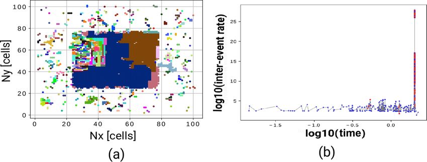
M. Monterrubio-Velasco et al.: The stochastic rupture earthquake model TREMOL v0.1 1811
(Gómez et al., 1998; Moral et al., 2001). 3 The TREMOL code
dU (t)
= −U (t)K(σ (t)), (1) Since the main objective of TREMOL is to simulate the rup-
dt ture process of seismic asperities based on the principles of
where U (t) is the number of fibers that remain unbroken at the FBM, we model two materials with different mechanical
time t. The hazard rate K(σ (t)) is a function of the fiber properties interacting with each other.
stress σ (t). Experimental results show that the hazard rate of In order to introduce the features of TREMOL we describe
materials under constant load can be well-described by the three main stages during the application of TREMOL.
Weibull probability distribution function. This behavior can
be summarized in Eq. (2) (Coleman, 1958; Phoenix, 1978; 1. Preprocessing
Phoenix and Tierney, 1983; Vázquez-Prada et al., 1999; In this stage we have to assign the following input data:
Moreno et al., 2001; Biswas et al., 2015): - the size of the fault plane,
σ (t) ρ
- the size of the maximum asperity within the fault
K(σ (t)) = ν0 , (2)
σ0 plane, and
where ν0 is the reference hazard rate, and σ0 the reference - other parameters (load-transfer value π , strength
stress. The Weibull exponent, ρ, quantifies the nonlinear- value γ , initial load values σ , and load threshold
ity (Yewande et al., 2003). If σ0 = ν0 = 1, the expression σth ).
in Eq. (2) can be simplified to K(σ (t)) = σ (t)ρ . From the 2. Processing
probabilistic formulation, two equations arise (Eqs. 3 and 4), TREMOL uses the data from the preprocessing stage to
which are applied in our algorithm to define the system dy- carry out the FBM algorithm, and by applying Eqs. (3)
namics. The details of these two equations are described be- and (4) the rupture process is computed in the fault
low. plane studied. The asperity size of each earthquake is
a) Gómez et al. (1998) and Moral et al. (2001) developed used by TREMOL to also compute the magnitude of
a relation to compute the expected rupture time (dimen- each synthetic earthquake.
sionless) of the fibers following Eqs. (1) and (2). This 3. Post-processing
expected rupture time interval is defined as δk (Eq. 3) In this stage, TREMOL summarizes the results that are
and can be applied to any load-transfer rule: computed in the processing stage and computes the
1 equivalent rupture area (km2 ). In general, TREMOL
δk = , (3)
N output generates a synthetic catalog of earthquakes,
ρ
X
σi (t) which consists of the following:
i=1
- total number of earthquakes that can occur in the
where N is the total number of cells, and σi is the load fault plane studied,
in the ith cell. The dimensionless cumulative time, T , is
the sum of δk . - size of the asperity of each earthquake, and
- magnitude of each earthquake.
b) The failure probability, Fi , which is a function of the
load σi in each cell, is (Moreno et al., 2001) In the next sections we describe with more detail each one
ρ of the three main stages during the application of TREMOL.
Fi = δk σi (t). (4)
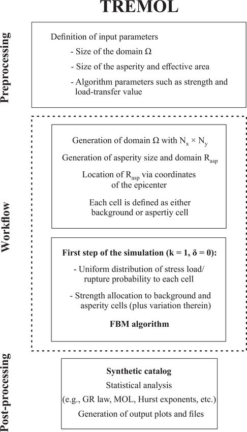
An overview of the entire simulation process is shown in
The dynamic values δk and Fi are updated with each Fig. 1.
time step due to rupture processes and the resulting load
transfer. 3.1 Preprocessing: input data and initial conditions
A suitable FBM algorithm to simulate earthquakes should In TREMOL, a fault plane is modeled as a rectangle (),
consider a complex stress field, physical properties of ma- which is divided into Nx ×Ny cells. Each cell is defined by its
terials, stress transfer between faults (at short and long dis- position (i, j ), where i ∈ [1, . . ., Nx ] and j ∈ [1, . . ., Ny ]. In
tances), and dissipative effects. Using the FBM we assume the fault plane earthquakes can occur with different mag-
that earthquakes can be considered analogous to character- nitudes. Additionally, it is possible to assign to each fault
istic brittle rupture of a heterogeneous material (Kun et al., plane an asperity region (RAsp ).
2006a, b). To define each fault plane () and its respective asperity
The previous basic concepts about the FBM were consid- region (RAsp ) it is necessary to assign specific properties to
ered for the development of the TREMOL code, with the pur- their cells. Particularly, it is necessary to define three proper-
pose of modeling the behavior of seismic asperities. In the ties (or values) for each cell of and RAsp : a load σ (i, j ), a
next section, we describe the details of this code. strength value γ (i, j ), and a load-transfer value π(i, j ).
www.geosci-model-dev.net/12/1809/2019/ Geosci. Model Dev., 12, 1809–1831, 2019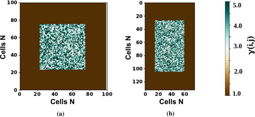
1812                                 M. Monterrubio-Velasco et al.: The stochastic rupture earthquake model TREMOL v0.1

                                                                          Figure 2. Schematic representation of the considered local load
                                                                          rule. The broken cell with load, σF , distributes the largest load frac-
                                                                          tion, σO (Eq. 5), to its four orthogonal neighbor cells. The remaining
                                                                          load, σD (Eq. 6), is transferred to its four diagonal neighbor cells.
                                                                          Afterwards, the load of the broken cell drops to zero, σ = 0. Asper-
                                                                          ity cells cannot receive any new load.

Figure 1. TREMOL flowchart. At the beginning (preprocess) the
algorithm initiates a domain  with Nx × Ny cells in which every
cell is either part of an asperity or of the background or fault plane.
Afterwards (first time step, k = 1) a uniform distribution allocates a
random stress load and rupture probability to all cells. In addition,
asperity cells obtain a random strength value from a uniform dis-
tribution. Next (time step k ≥ 2) the failure process starts following    Figure 3. (a) Spatial distribution of the random initial loads σ (i, j ).
the FBM algorithm. After every failure the stress of the broken cell      RAsp represents a rectangular fault plane of Nx = Ny = 100 cells.
is redistributed via the LLS rule and the number of time steps (k) in-    The color bar indicates the load and the threshold load of σth = 1.
creases by 1 until the target number of time steps is reached. If the     (b) Spatial distribution of the strength γ (i, j ). Two main regions
final number of time steps has been reached the simulation stops.         can be distinguished in this figure: (1) the asperity region defined as
At the end, all information about the entire failure process is saved     the inner rectangle and (2) a background area or fault plane. While
in a database or a synthetic catalog that can be used for statistical     the asperity contains strength values in the range of 3 to 5, the rest
analysis. Further details about the algorithm are given in Sect. 3.       of the fault plane has a strength value of 1.

                                                                             – The strength value γ (i, j ). This parameter represents an
  – The load σ (i, j ). At the beginning of each realization,                  analogy to the concept of hardness or strength. In our
    TREMOL randomly assigns a value of the load σ (i, j )                      model, the algorithm will find it difficult to break a cell
    to each cell of  using a uniform distribution function                    if this cell has a value γ > 1 since the strength threshold
    (0 < σ (i, j ) < 1). This assumption simulates a hetero-                   before failure is set as γth = 1 (see a detailed explana-
    geneous stress field. Moreover, a load threshold σth = 1                   tion in Sect. 3.2). As a result, a strength γ > 1 may sim-
    is necessary to create a limit at which a cell must fail                   ulate a hard material that needs to be weakened before it
    (Moreno et al., 2001). At the end of this step any cell                    can fail. This process can be regarded as similar to ma-
    within  must have a load value between 0 and 1.                           terial fatigue or creep failure. The strength value for all

Geosci. Model Dev., 12, 1809–1831, 2019                                                       www.geosci-model-dev.net/12/1809/2019/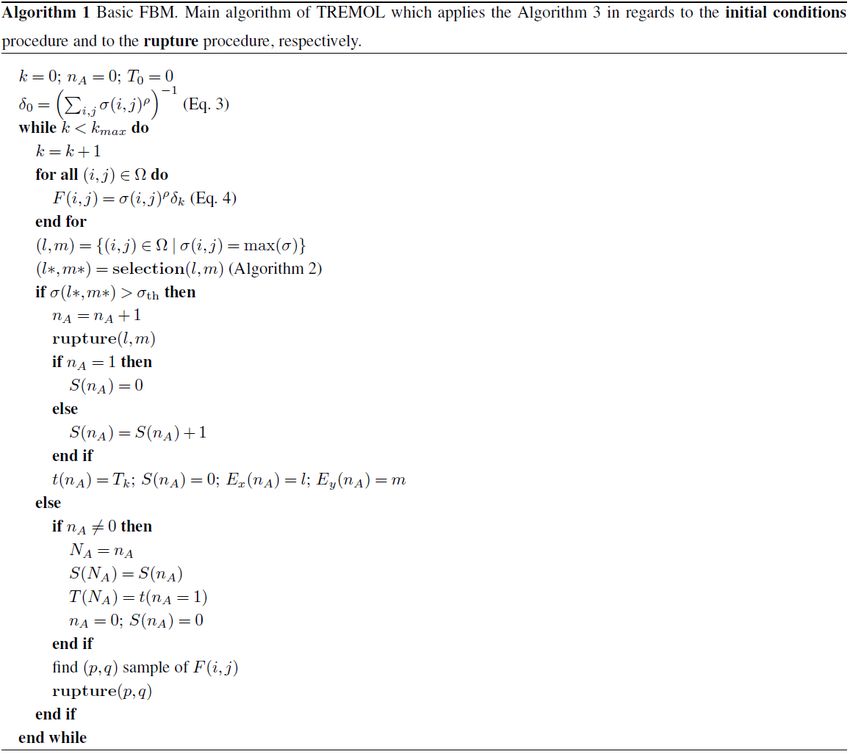
M. Monterrubio-Velasco et al.: The stochastic rupture earthquake model TREMOL v0.1 1813
cells in RAsp , namely γAsp , is chosen in a discrete inter- – Avalanche event. If one or more cells have a load value
val of UD = [γRef − 1, γRef + 1], where UD is an integer σ (i, j ) ≥ σth , an avalanche event is generated, and the
uniformly distributed and γRef is an assigned reference cell that fails is the one with the greatest σ (i, j ) value.
value.
Due to the integrated strength property some extra rules
– The load-transfer value π(i, j ). This parameter repre- for rupture are necessary. The requirement for failure is
sents the percentage of load that can be distributed from γ (i, j ) = 1. On the other hand, if a cell with γ (i, j ) > 1 is
a ruptured cell to its neighbors. In this study, the load chosen, its strength is reduced by one unit. This strength con-
in the ruptured cell is called σF (i, j ). TREMOL uses dition enables us to simulate a material weakening process
a local load sharing (LLS) rule considering the eight during the load-transfer process. Additionally, this condition
nearest neighbors. According to previous studies, such offers the possibility to produce large load accumulations lo-
as Monterrubio-Velasco et al. (2017), TREMOL redis- cally, which are more likely to generate larger ruptures.
tributes the majority of the load to the four orthogonal When a cell within RAsp breaks it becomes inactive until
neighbors. The load that is transferred to these orthog- the end of the simulation, which means it cannot receive any
onal neighbors is called σO , and it is defined according further load. The large load concentration within the asperity
to Eq. (5): usually produces a very short time interval (Eq. 3), with the
result that there is physically not enough time available to
0.98σF (i, j )πF (i, j )
σO (i, j ) = , (5) reload the stress on an asperity right after its rupture. On the
4 contrary, a cell outside of the asperity region remains active
where πF is the load-transfer value of the failed cell. Ad- after its failure but its load drops to zero. The simulation ends
ditionally, a small proportion of the load is transferred when all the cells within the asperity have become inactive.
to the four diagonal neighbors. The value of this load is
called σD (i, j ), and it is defined according to Eq. (6): 3.3 Output data and post-processing
0.02σF (i, j )πF (i, j ) After every execution TREMOL outputs a catalog detail-
σD (i, j ) = . (6)
4 ing where the position (x, y) of the failed cell, the rupture
The assumption of Eqs. (5) and (6) is in agreement with time (Eq. 12), the avalanche event or normal event identi-
what is expected for the maximum shear stress direc- fication, the mean load, and many other values are saved
tions with respect to the main stress orientation that for each time step. We cluster avalanche events considering
gives rise to both synthetic and antithetic faulting (e.g., the time and space criterion. We assume ai−1 = (xi−1 , yi−1 )
Stein and Wysession, 2008). Figure 2 is a schematic and ai = (xi , yi ) are two consecutive avalanche events gen-
representation of the load distribution process from the erated in chronological√order. If their Euclidean distance is
failed cell, σF (i, j ) (in red), to its nearest neighbors. 1ri ≤ rth (where rth = 2 2), then ai and ai−1 will belong to
the same cluster. This clustering algorithm is applied to all
In order to differentiate the parameters of the asperity generated avalanche events. Lastly, we extract a new catalog
from the rest of the fault plane , we define πAsp (i, j ) and that shows the size of each cluster, the position of the first
γAsp (i, j ) that refer only to the cells within RAsp . For the element of each cluster related to the nucleation point, and
rest of the fault plane , we are using the same parameters the time when it was initiated. This database is our simulated
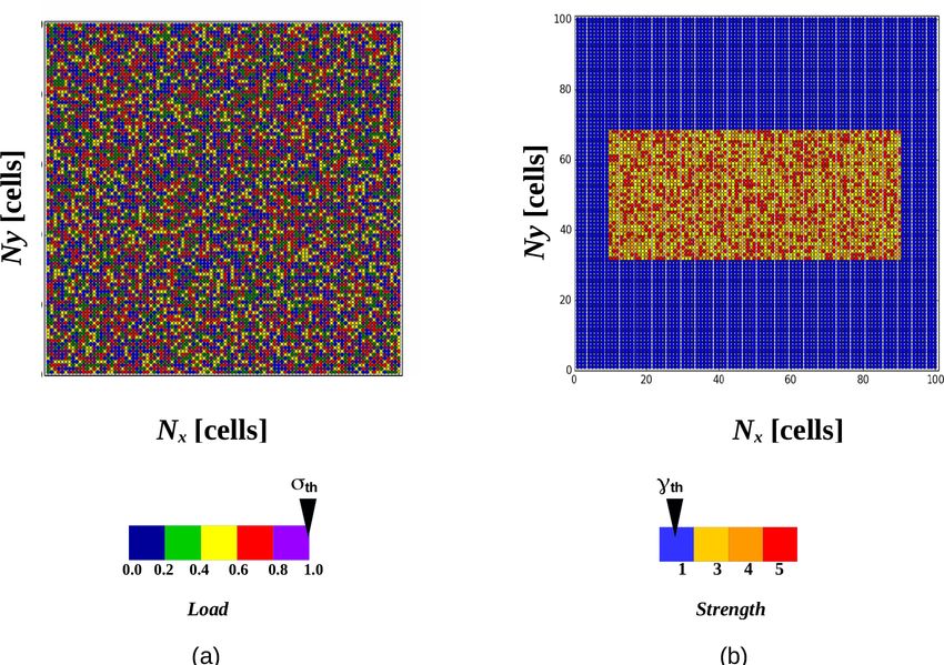
defined previously: π(i, j ) and γ (i, j ). Figure 3a shows an seismic catalog. Note that the cluster size is given in nondi-
example of the randomly distributed initial load throughout mensional units. However, we use an equivalence between
the fault plane. Figure 3b displays an example of differences and an effective area Aeff in order to obtain a physical rupture
between the strength of the asperity and the rest of the fault area. Finally, each cell can represent an area in square kilo-
plane. meters. This step is necessary in order to compute an equiv-
alent magnitude, which is comparable with real earthquake
3.2 Main computational processes
magnitudes. For this purpose, we use three magnitude–area
Once the initial information for the entire domain is de- relations. In particular, we use Eqs. (7), (8), and (9) obtained
fined, the core algorithm of TREMOL will realize a transfer, by Rodríguez-Pérez and Ottemöller (2013) for Mexican sub-
accumulation, and rupture process. While the cells interact duction earthquakes:
with each other, there are two basic failure processes depend- log10 Aa = −4.393 + 0.991M w , (7)
ing on the load of the cell in comparison with the threshold
log10 Aa = −5.518 + 1.137M w , (8)
load (Moreno et al., 2001).
log10 Aa = −6.013 + 1.146M w , (9)
– Normal event. If all cells within the system have a load
σ (i, j ) < σth , a normal event is generated, and the cell where Aa is the asperity area (km2 ). Equation (7) was ob-
that will fail is randomly chosen considering the indi- tained from asperities defined by the average displacement
vidual failure probability of each cell, F (i, j ) (Eq. 4). criterion (Somerville et al., 1999). Equations (8) and (9) were
www.geosci-model-dev.net/12/1809/2019/ Geosci. Model Dev., 12, 1809–1831, 2019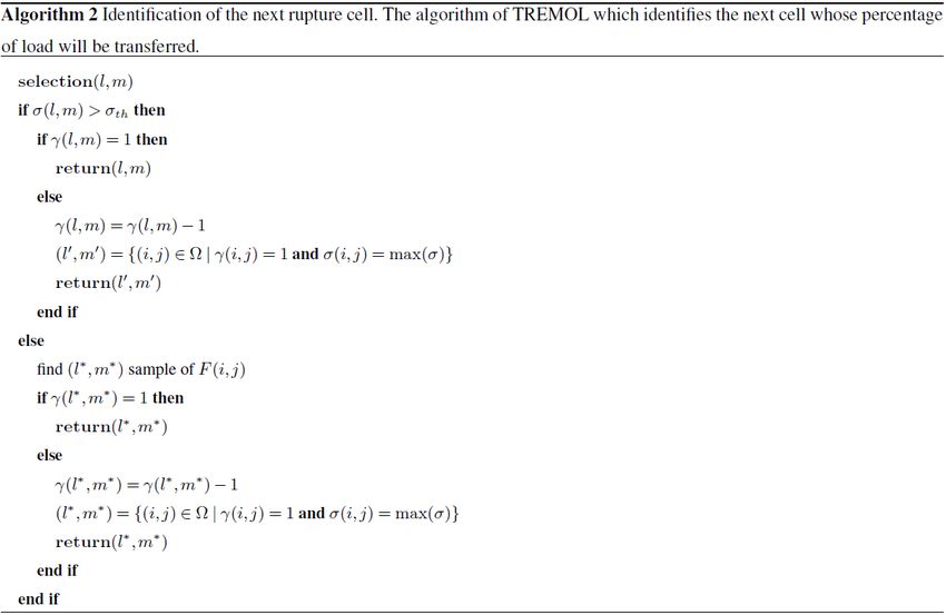
1814                               M. Monterrubio-Velasco et al.: The stochastic rupture earthquake model TREMOL v0.1

Figure 4. Results of one realization by TREMOL. (a) The spatial distribution of avalanches. Patches of the same color indicate one temporal-
consecutive Avalanche cluster (synthetic earthquake). (b) Logarithmic representation of the inter-event rate with time. The red dots represent
the inter-event rate when the asperity rupture occurs. The blue dots indicate foreshocks.

computed from asperities defined by the maximum displace-                   The flowchart in Fig. 1 and the pseudo-codes 1, 2, and
ment criterion for a large asperity and a very large asperity,           3 summarize the algorithm of TREMOL. A summary of all
respectively (Mai et al., 2005).                                         required parameters to execute the TREMOL code are shown
   Furthermore, we define the inter-event rate 1νk as analo-             in Table 1.
gous to the rupture velocity:
        1rk                                                              4     Sensitivity analysis
1νk =       ,                                                  (10)
        1δk
                                                                         4.1     Methods: parametric study
where 1rk is the inter-event Euclidean distance between the
k event located at (xk , yk ) and k − 1 event in (xk−1 , yk−1 ).         We performed a sensitivity analysis of the three asperity pa-
       q                                                                 rameters (γasp , Sa−Asp , and πasp ) in order to identify the best
1rk = (xk − xi−k )2 + (yk − yi−k )2                          (11)        combination that produces the best approximation to real
                                                                         data, such as the maximum rupture area, Asyn , and its re-
The inter-event time 1δk is computed following                           lated magnitude Msyn . In order to investigate the influence of
1δk = δk − δk−1 ,                                              (12)      every single parameter, we statistically determined how the
                                                                         results vary with different parameter configurations.
where δk is given by Eq. (3). Figure 4a shows an example
of the final spatial distribution of rupture clusters for a par-         4.1.1    Percentage of transferred load, πasp – methods
ticular example. Each cluster is indicated by the same color
and represents a simulated earthquake. Figure 4b shows the               To explore the influence of πasp , we analyzed 12 values
related inter-event rate. The inter-event rate largely increases         (0.67 ≤ πasp ≤ 1.0, with increments of 0.3). The minimum
when the asperity rupture occurs.                                        πasp = 0.67 assigns the same value to an asperity cell and to
   In the post-processing step we additionally computed the              a background cell. On the other hand, πasp = 1.0 means that
rupture duration of the largest simulated earthquake, DAval ,            the load in a failed asperity cell is fully transmitted to the
using the rupture velocity and the effective fault dimensions            neighbors (ideal case with no dissipative effects). Note that
obtained from finite-fault models (Table 5).                             πasp = 1 does not represent real physical conditions since
   We used Eq. (13) (Geller, 1976) to compute DAval :                    dissipative effects are ignored completely. On the other hand,
                                                                         if πasp = 0.67 (case 1) the asperity cells would transfer as
                      √
          LMax 16 WMax × LMax                                            much load as the cells in the background. The objective is to
DAval =         +                      ,                    (13)         generate a load concentration within the asperity that corre-
           Vr            7π 3/2 β
                                                                         sponds to the largest magnitude. If the asperity cells trans-
where                                                                    fer as much load as the background cells, no such load con-
      Vr                                                                 centration can be obtained. As a result, we can expect that
β≈        .                                                    (14)      the mean Asyn for πasp = 0.67 (case 1) is the lowest value in
     0.72
                                                                         comparison to all other cases.
  Using these considerations, we can assign a physical                      The input data of this experiment are summarized in Ta-
unit of time (s) to the largest simulated earthquake, Asyn =             ble 2. We assigned a strength to the asperity (RAsp ) γasp =
LMax × WMax .                                                            4 ± 1 and a value of γBkg = 1 to the rest of the fault plane.

Geosci. Model Dev., 12, 1809–1831, 2019                                                      www.geosci-model-dev.net/12/1809/2019/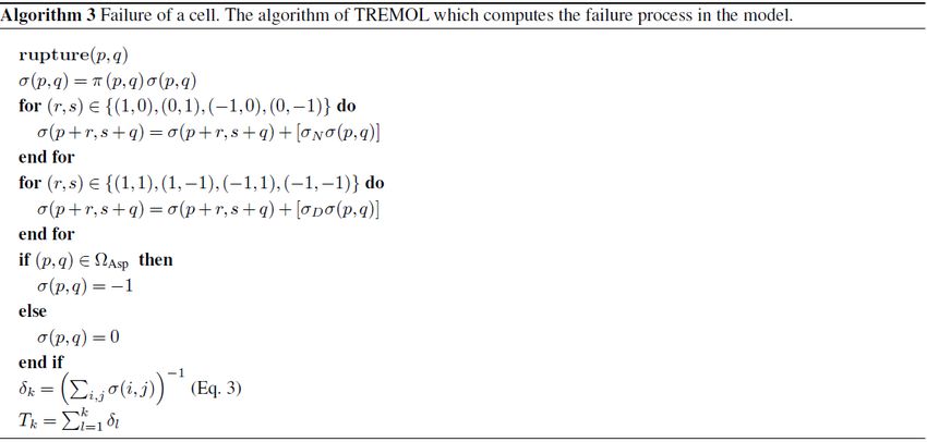
M. Monterrubio-Velasco et al.: The stochastic rupture earthquake model TREMOL v0.1                                                   1815

Table 1. TREMOL preprocessing: input parameters and their definition.

                          Parameter    Definition
                          Ncell        number of cells in
                          πasp         percentage of transferred load to neighbor cells in the asperity domain
                          γasp         strength at each (i, j ) cell in the asperity domain
                          Sa−Asp       ratio of asperity area computed by TREMOL
                          Sa           ratio of asperity area computed by finite-fault model
                          Aeff         effective area (km2 ) computed by finite-fault model
                          Aa           asperity area (km2 ) computed by finite-fault model

These values are chosen after experimental trials, which                load configurations, σ(i,j ) , to ensure that the results over πasp
have shown that the difference is large enough to sim-                  are independent of the initial load conditions σ(i,j ) .
ulate a significant strength difference with low computa-
tional effort. To define the effective area and the asper-
                                                                        4.1.2   Strength parameter, γasp – methods
ity size, we chose the values computed for the earthquake
of 20 March 2012, M w = 7.4, in Rodríguez-Pérez and Ot-
temöller (2013): Aeff = 2944.2 km2 and Sa = 0.26. We de-                To perform the parametric study of γasp , we configured two
fined the size of  consisting of Ncell = 10 000 cells in total.        asperities embedded in . In this experiment, the total size
We carried out 50 simulations per πasp configuration. In ad-            is  = 200 × 100 cells. Afterwards, we located each asperity
dition, we modified the random seed to have different initial           in the center of the two sub-domains 0 of 100 × 100 cells.
                                                                        Figure 5 shows a schematic representation of the domains
                                                                        and 0 used in this experiment.

www.geosci-model-dev.net/12/1809/2019/                                                     Geosci. Model Dev., 12, 1809–1831, 2019
1816 M. Monterrubio-Velasco et al.: The stochastic rupture earthquake model TREMOL v0.1
The separation between the two asperities remains con- fined the same asperity size for both: Sa1 = Sa2 = 0.22. In
stant. We chose a value of πasp = 0.90 to produce a large Fig. 6, we show an example of the spatial configuration of
contrast between the asperity and the rest of the fault plane this analysis. The background strength is considered to be
(π = 0.67) (Monterrubio-Velasco et al., 2017). In order to γbkg = 1 = constant, and the color bar indicates the γ (i, j )
analyze the influence of γasp (and Sa−Asp ), the asperity on the values.
right-hand side (Asp. 2) has varying strength values, while
the strength of the left asperity (Asp. 1) remains constant. Fi- 4.1.3 Asperity size, Sa−Asp – methods
nally, the maximum ruptured area and magnitude generated
in each 0 are computed. The modification of the Sa−Asp parameter was based on the
In order to explore how the system behaves when γasp same configuration as described in the previous section. We
changes, we analyzed six different values of γasp = [2±1, 5± analyzed six different values of the asperity size Sa (cases 19
1, 7 ± 1, 9 ± 1, 11 ± 1, 14 ± 1] (cases 13 to 18). The input to 24). In Fig. 7 we show an example of the asperity con-
data used in this test are summarized in Table 3. We de- figuration in which the left asperity (Asp. 1) has a constant
size Sa2 , while the size of the right one (Asp. 2) increases. In
Geosci. Model Dev., 12, 1809–1831, 2019 www.geosci-model-dev.net/12/1809/2019/M. Monterrubio-Velasco et al.: The stochastic rupture earthquake model TREMOL v0.1 1817
Table 2. Input data in order to carry out cases 1 to 12. Table 3. Main input data in order to carry out cases 13 to 18.
Data Value Data Value
Number of 1 Number of asperities 2
asperities
γasp 2 ± 1(case 13), 5 ± 1(case 14),
πasp 0.67 (case 1), 0.70 (case 2), 0.73 (case 3), 7 ± 1(case 15), 9 ± 1(case 16),
0.76 (case 4), 0.79 (case 5), 0.82 (case 6), 11 ± 1(case 17), 14 ± 1(case 18)
0.85 (case 7), 0.88 (case 8), 0.91 (case 9),
Ncell 20 000
0.94 (case 10), 0.97 (case 11),
πasp 0.90
and 1.0 (case 12).
πbkg 0.67
Number of 50 γbkg 1
realizations σth 1
Sa1 0.22
Ncell 10 000
Sa2 0.22
γasp 4±1
Aeff 2944.2 (km2 )
π 0.67
γ 1
σth 1
Sa 0.26
Aeff 2944.2 (km2 )
Figure 5. Schematic configuration for the parametric study of γasp Figure 6. Example of the strength configuration γ (i, j ) for the sen-
and Sa−Asp . The size of the domain is = 200 × 100 cells. Each sitivity analysis of γasp . Two asperities with the same size Sa−Asp =
asperity is located within the center of the two sub-domains 0 of 0.22 are defined and embedded in following the schema in Fig. 5.
100 × 100 cells. The strength parameter γasp and degree of hetero- The conservation parameters are πasp = 0.90 and πasp = 0.67. The
geneity for each asperity can be varied according to the material color bar indicates different γ (i, j ) values. The left asperity (Asp. 1)
properties. contains constant properties, while the right asperity (Asp. 2) has
variable strength values.
this experiment, we considered γasp = 5 ± 1 and πasp = 0.90.
The main data related to these six cases are summarized in latter, the database provides estimations of effective fault di-
Table 4. mensions, rupture velocity, source duration, number of asper-
ities, stress, and radiated seismic energy on the asperities and
4.2 Model validation – methods background areas. Slip solutions were obtained with teleseis-
mic data for events with 6.4 < M w < 8.2.
We evaluated the capability of the model to reproduce the The number of cells was Ncell = 10 000 for a domain of
characteristics of 10 Mexican subduction earthquakes (eight 100 × 100 cells. We modeled the size of proportionally to
shallow thrust subduction events, ST, and two intra-slab sub- the size of Leff and Weff for each scenario according to the
duction events, IN). The input data of the effective area, following equations, Eqs. (15) and (16):
Aeff , and the asperity ratio size, Sa , are given from waveform
slip inversions and seismic source studies (Aeff = Leff × Weff
and Sa = Aa /Aeff ) shown in the database of Mexican earth-
quake source parameters by Rodríguez-Pérez et al. (2018).
This database includes results from two different method-
ologies: spectral analysis and finite-fault models. From the
www.geosci-model-dev.net/12/1809/2019/ Geosci. Model Dev., 12, 1809–1831, 20191818 M. Monterrubio-Velasco et al.: The stochastic rupture earthquake model TREMOL v0.1
Table 4. Main input data in order to carry out cases 19 to 24.
Data Value
Number of asperities 2
Ncell 20 000
πasp 0.90
γasp 5±1
πbkg 0.67
γbkg 1
σth 1
Sa2 0.22 (case 19),0.28 (case 20), Figure 8. Example of the domain configuration , considering Leff
0.34 (case 21), 0.40(case 22), and Weff . (a) Example configuration of event 3 and (b) example
0.46 (case 23), 0.52 (case 24) configuration of event 5. The required data can be found in Table 5.
Sa1 0.22
In future trials it may be useful to consider the inner uncer-
tainties of finite-fault models. The asperity aspect ratio fol-
Nx(Sa)
lows the same proportion as the effective area, x
y = Ny(Sa)
(Fig. 8).
We carried out 50 realizations per event (Table 5), chang-
ing the size Sa−Asp in each one (Eq. 17).
4.2.1 Modeling the rupture area and magnitude of 10
subduction earthquakes – methods
In this case the number of cells is Ncell = 10 000 (100×100).
We carried out 50 executions per event and in each execution
we randomly changed the size Sa−Asp following Eqs. (15),
(16), and (17). The input data of the 10 modeled earthquakes
in Table 5 are summarized in Table 6.
Figure 7. An example configuration of different asperity sizes, 4.2.2 Case study (Oaxaca, M w = 7.4, 20/03/2012):
Sa−Asp . The color bar indicates the strength γ (i, j ) values used dur- using different effective areas Aeff for the same
ing the test. event – methods
As reported in Rodríguez-Pérez et al. (2018) for some events,
there are several solutions that allow us to analyze the vari-
ability in the estimated source parameters (see parameters of
s
Ncell Leff
Nx = , (15) events 7, 7a, and 7b in Table 5). In this study, we applied
Weff TREMOL to study how the ruptured area and the assessed
Weff magnitude change when we use different input data to model
Ny = Nx , (16)
Leff the same earthquake. The data related to these three events
are summarized in Table 7.
where Nx and Ny are the number of cells in the x axis and
y axis, respectively. As an example, Fig. 8 presents the size 4.2.3 Assessing a future earthquake in the Guerrero
and aspect ratio of Ev. 3 and Ev. 5 (Table 5). seismic gap: rupture area and magnitude –
In some cases, the number of asperities computed in methods
Rodríguez-Pérez et al. (2018) is greater than 1. However, as
a first approximation we simplified the problem by modeling We apply our method for the estimation of possible future
only one asperity per earthquake. earthquakes, in particular to compute the expected magni-
In order to study how the asperity size Sa affects the max- tude, since TREMOL may offer new insights for future haz-
imum ruptured area, we randomly modified the size as ard assessments. We carried out a statistical test to assess the
Sa−Asp = Sa + (α · (Sa /2)), (17) size of an earthquake that may occur in the Guerrero seismic
gap (GG) region.
where 0 < α < 1 is a random value. We introduce this as- As input parameters, we used the area found by Singh and
sumption because we want to avoid a preconceived final size. Mortera (1991): Leff = 230 km × Weff = 80 km. We defined
Geosci. Model Dev., 12, 1809–1831, 2019 www.geosci-model-dev.net/12/1809/2019/M. Monterrubio-Velasco et al.: The stochastic rupture earthquake model TREMOL v0.1 1819
Table 5. The finite-fault source parameters used in this work. Weff and Leff are the effective fault dimensions (width and length, respectively,
according to Mai and Beroza, 2000). Areal is the asperity area, Aeff is the effective rupture area (Weff ×Leff ). Duration is the rupture duration
computed from the slip inversion, Na is the number of asperities, and Vr is the rupture velocity. Ratio is the aspect ratio of the fault area. The
type of the event is labeled ST for shallow thrust and IN for intra-slab events.
Ev. Date Mw Leff Weff Ratio Sa = Duration Vr Type Na Reference
ID (km) (km) Areal /Aeff (s) (km S−1 )
1 07/06/1982 7.0 34.47 17.81 1.94 0.23 – 3.2 ST 1 Rodríguez-Pérez and Zúñiga (2016)
2 19/09/1985 8.1 158.62 115.04 1.38 0.31 – 2.6 ST 2 Mendoza (1989)
3 30/04/1986 6.8 38.31 37.16 1.03 0.26 22 2.5 ST 1 Rodríguez-Pérez and Ottemöller (2013)
4 14/09/1995 7.4 68.80 46.61 1.48 0.23 32 2.5 ST 1 Rodríguez-Pérez and Ottemöller (2013)
5 09/10/1995 8.0 169.65 59.25 2.86 0.27 92 2.8 ST 2 Rodríguez-Pérez and Ottemöller (2013)
6 18/04/2002 6.7 23 13.88 1.66 0.24 30 2.2 ST 2 Rodríguez-Pérez and Ottemöller (2013)
7 20/03/2012 7.4 54.94 53.59 1.03 0.26 30 2.7 ST 1 Rodríguez-Pérez and Ottemöller (2013)
7a 7.4 51.42 55.47 0.93 0.21 – 1.8 ST 1 USGS
7b 7.4 40.03 44.60 0.89 0.21 – 2.0 ST 1 Wei (2012)
8 11/04/2012 6.5 21.95 21.84 1.04 0.23 15 2.8 ST 1 Rodríguez-Pérez and Ottemöller (2013)
9 08/09/2017 8.2 125.95 71.13 1.77 0.34 – 2.0 IN 3 USGS
10 19/09/2017 7.1 34.47 36.12 0.95 0.32 – 2.2 IN 1 USGS
Table 6. Main data used for Ev. 1 to Ev. 10. Table 8. Main data for assessing a future earthquake in the Guerrero
seismic gap (GG event).
Data Value
Number of asperities 1 Data Value
Ncell 10 000 Number of asperities 1
πasp 0.90 Ncell 10 000 (cells)
γasp 5±1 πasp 0.90
πbkg 0.67 γasp 5±1
γbkg 1 πbkg 0.67
σth 1 γbkg 1
Sa see Table 5 σth 1
Sa−Asp Eq. (17) Sa−Asp Eq. (17)
Aeff see Table 5 Sa 0.25
Aeff 18 400 (km2 )
Table 7. Main data for the case study Ev. 7 test, Ev. 7a test, and
Ev. 7b test.
Sa ), we executed the algorithm as in previous sections. The
Data Value input data related to this analysis are summarized in Table 8.
Number of asperities 1 Likewise, we want to estimated the duration Daval of the
Ncell 10 000 (cells) event. To compute this value, we used a mean of the Vr from
πasp 0.90 Table 5.
γasp 5±1
πbkg 0.67
γbkg 1
σth 1 5 Results
Sa−Asp Eq. (17)
Sa see Table 5 (Ev. 7, 7a, and 7b) 5.1 Results: parametric study
Aeff see Table 5 (Ev. 7, 7a, and 7b)
5.1.1 Percentage of transferred load, πasp
the asperity size ratio Sa as proposed by Somerville et al. Figure 9 shows the mean (black dots) of the maximum rup-
(2002) for regular subduction zone events (SB) based on av- tured area Asyn , including the upper and lower limits of the
erage slip, Sa = 0.25. Singh and Mortera (1991), Astiz et al. standard deviations (blue squares), after the execution of all
(1987), and Astiz and Kanamori (1984) proposed a proba- 12 cases (Table 2) with 50 realizations. The value of Asyn is
ble maximum magnitude for this region of M w ≈ 8.1 − 8.4. related to the largest produced cluster in . There are two
Therefore, using the effective rupture area (Leff , Weff , and dominant tendencies identifiable.
www.geosci-model-dev.net/12/1809/2019/ Geosci. Model Dev., 12, 1809–1831, 20191820 M. Monterrubio-Velasco et al.: The stochastic rupture earthquake model TREMOL v0.1
2. If 0.70 ≤ πasp < 0.76, a transition with an increasing
trend with the largest standard deviation is visible.
3. If πasp = 0.67 (case 1), the mean of the maximum mag-
nitude is the lowest.
In this experiment, the initial value of Sa = 0.26 remains con-
stant; i.e., the asperity size does not increase randomly (red
line in Fig. 11). After executing all configurations, we com-
puted the ratio of Sa−Asp = Asyn /Aeff , relating to the largest
ruptured area. We show the mean and standard deviation of
this ratio Sa−Asp in Fig. 11. We observed that the ratio of
Sa−Asp is always ≈ 0.10 lower than Sa .
Figure 9. Mean of the maximum rupture area (km2 ), Asyn , for dif- 5.1.2 Strength parameter, γasp
ferent values of πasp depicted as black circles. The minimum and
maximum limits of the rupture area are represented by blue squares. For each value of γasp (Table 3), we performed 50 executions
while changing the initial strength parameter of the asperity
γasp (Fig. 3b). Likewise, we computed the maximum mag-
nitude obtained for each 0 . Figure 12 indicates the mean
and standard deviation of the computed maximum magnitude
with a dependence on γasp . The upper subplot (blue markers)
shows the results for the left (constant) asperity (Asp. 1). The
lower subplot (red markers) shows the results for the right
(variable) asperity (Asp. 2).
We observe in Fig. 12 that the mean magnitude remains
essentially independent for γasp > 5±1. Additionally, the er-
ror bars slightly decrease, while γasp increases. Another ob-
servation is that when γasp = 2 ± 1 the average of the max-
imum magnitude is the lowest in both asperities. Moreover,
there is a transition zone for 2 ± 1 ≤ γasp ≤ 5 ± 1. We ob-
served that γasp > 5 ± 1 has a limited influence on the re-
Figure 10. Mean and standard deviation of the maximum magni- sults of the maximum magnitude. The maximum magnitude
tude over 50 realizations depending on πasp .
of γasp = 14 ± 1 is approximately 0.3 magnitudes larger than
the one of γasp = 5 ± 1.
1. If πasp < 0.76, the mean of the maximum ruptured area 5.1.3 Asperity size, Sa−Asp
increases continuously more than 1 order of magnitude
from 15 to ≈ 500 km2 , i.e., an increase of 3333 %. The Figure 13 shows the mean magnitude and standard devia-
standard deviation of Asyn for πasp = 0.7 is ≈ 35 km2 tion as a function of asperity size. The first asperity with the
(100 % error). fixed size indicates a relatively constant magnitude of ap-
proximately 7.4. Conversely, the second asperity with vari-
2. If πasp ≥ 0.76 (cases 4 to 12), the Asyn values remain es- able size produces only a slight increase in magnitude. The
sentially constant (≈ 500 km2 ). Likewise, the upper and magnitude of Sa−Asp = 0.52 is approximately 0.5 magni-
lower limit vary around the same order. The standard tudes larger than the one of Sa−Asp = 0.22.
deviation for this interval is ≈ 100 km2 (20 % error).
5.2 Results: model validation
Using the mean of Asyn obtained in each case, we com-
puted the corresponding magnitude. The results are given as 5.2.1 Modeling 10 Mexican subduction zone
the mean and standard deviation of the maximum magnitude earthquakes
in Fig. 10 for all 12 cases (see Table 2). Due to the fact that
ruptured area and magnitude are correlated (see Eqs. 7, 8, and Based on the observations described in the previous sec-
9), the pattern in Fig. 10 is very similar to the one in Fig. 9. tion, we used γasp = 5 ± 1 and πasp = 0.90 in order to val-
Overall, there are three aspects observable. idate the model. We chose γasp = 5 ± 1 because it repre-
sents the strength interval of 5 ± 1 ≤ γasp ≤ 14 ± 1 with less
1. If πasp ≥0.76 (cases 4 to 12), the mean magnitudes show computational cost. We chose πasp = 0.90 because it rep-
a steady value (≈ 7.2). resents the relatively constant magnitude for the parameter
Geosci. Model Dev., 12, 1809–1831, 2019 www.geosci-model-dev.net/12/1809/2019/M. Monterrubio-Velasco et al.: The stochastic rupture earthquake model TREMOL v0.1 1821 Figure 11. Mean and standard deviation of the ratio Ssyn = Asyn /Aeff over 50 realizations for different values of πasp . The red line indicates the asperity ratio Sa computed for event 7 (Table 5). Figure 12. Statistical results of γasp for a configuration similar to Fig. 6. Markers represent the mean value, while the error bars indicate the standard deviation for all 50 executions considering different initial strength configurations. The red markers correspond to the results of the left asperity (Asp. 1) and blue markers to the results of the right asperity (Asp. 2) (Fig. 6). The strength of the left asperity is kept constant, whereas the strength of the right asperity is variable. range 0.76 ≤ πasp ≤ 0.90. In addition, πasp = 0.90 enables majority of earthquakes. Only three events show significant us to obtain the best approximation to the ratios of Sa−Asp . differences between synthetic and realistic maximum rupture Both parameter choices ensure an appropriate reproduction area. Even in these cases, however, Areal is located within the of the asperity rupture area, the maximum magnitude, and upper and lower limit of Asyn . least computational payload. Figure 15 shows the statistical results of the synthetic max- Figure 14 depicts a comparison between the (real) asper- imum magnitude, Msyn , determined for all 10 events. The ity area Areal (Table 5) and the area of the largest simulated real magnitudes from Table 5 are given as red markers. Black earthquake, Asyn . We plot the mean (blue dots), the minimum circles indicate the mean of Msyn of 50 realizations using (green triangles), and the maximum (red triangles) of all 50 Eq. (7), whereas blue and green markers indicate the mag- realizations for each real earthquake event. Black squares nitude following the Eqs. (8) and (9), respectively. The error represent the real asperity size. The results in Fig. 14 point bars represent the standard deviation. We observed that the out that Asyn is almost identical to Areal from Table 5 for the statistical parameters computed with TREMOL fit the mag- www.geosci-model-dev.net/12/1809/2019/ Geosci. Model Dev., 12, 1809–1831, 2019
1822                               M. Monterrubio-Velasco et al.: The stochastic rupture earthquake model TREMOL v0.1

Figure 13. Statistical results of Sa−Asp for a configuration similar to Fig. 7. The markers indicate mean and standard deviation for 50
realizations. Red markers correspond to the results of the right and variable asperity and blue markers to the results of the left and stable
asperity.

Figure 14. Comparison between the real asperity area Areal and the synthetic values (mean and standard deviation) of the largest ruptured
event Asyn . Black squares depict the real asperity area from Table 5, whereas blue circles indicate the mean area of 50 executions. Red and
green triangles represent the maximum and minimum Asyn .

nitudes shown in Table 5. However, the computed magni-                   results of assessing the magnitude by means of TREMOL us-
tudes depend on the scale relation employed (Eqs. 7, 8, and              ing a randomly modified asperity size, Sa−Asp (Eq. 17), are
9). Figure 16 includes the mean of the three scale relations.            reasonable.
Overall, the mean magnitude M syn and the expected magni-                   Figure 17 shows the real ratio size Sa from Table 5 (black
tude M w show similar values. Given that the difference be-              squares) in comparison to the mean of the largest simulated
tween the mean and the expected value (Table 5) is lower                 earthquake, Ssyn (blue squares). The standard deviation is
than 1M w < 0.5 for the 10 events, we can confirm that the               represented as error bars. The results indicate that in most of

Geosci. Model Dev., 12, 1809–1831, 2019                                                     www.geosci-model-dev.net/12/1809/2019/
M. Monterrubio-Velasco et al.: The stochastic rupture earthquake model TREMOL v0.1                                                     1823

Figure 15. Statistical results of the maximum magnitude for the events from Table 5. Red squares depict the real estimated magnitudes from
Table 5, while black circles, blue triangles, and green triangles represent the synthetic mean magnitude of 50 executions following Eqs. (7),
(8), and (9), respectively. The error bars are the standard deviation of the scale relations.

Figure 16. Statistical results of the maximum magnitude for the events from Table 5. Red squares represent the magnitudes from Table 5,
whereas black circles represent the mean magnitude (M syn ) value of all 50 executions following Eqs. (7), (8), and (9). The error bars stand
for the standard deviation of the mean for the three scale relations.

the cases the computed Ssyn range fits the expected Sa well.             ployed strategy of randomly increasing asperity size (using
Note that for events 3, 7, and 8 the mean values are lower than          Eq. 17) generates rupture areas similar to the ones proposed
the reported Sa , while Ssyn is overestimated for events 2, 5,           by Rodríguez-Pérez et al. (2018).
and 9. For events 1, 4, 6, and 10 the estimated value of Ssyn               We also computed an equivalent rupture duration, DAval ,
coincides with the expected one. However, the error bars en-             using the equation proposed by Geller (1976) to calculate the
compass the expected values in all cases (Fig. 17). Moreover,            rise time (Eqs. 13 and 14). Rodríguez-Pérez and Ottemöller
if we compare Fig. 17 with Fig. 11 we observe that the em-               (2013) determined the rupture velocity Vr (Ev. 3–8), which is

www.geosci-model-dev.net/12/1809/2019/                                                       Geosci. Model Dev., 12, 1809–1831, 2019
1824                               M. Monterrubio-Velasco et al.: The stochastic rupture earthquake model TREMOL v0.1

Figure 17. Proportion of simulated ruptured area occupied by the largest avalanche, Ssyn , in comparison with the real ratio size Sa from
Table 5. The real ratio size Sa from Table 5 is represented by black squares and the mean of the largest simulated earthquake, Ssyn , by blue
squares. The standard deviation is represented as error bars.

a useful parameter in order to validate our results. Figure 18           combinations express similar results, the closest approxima-
shows the results of this analysis. In red we plot the values            tion between real and synthetic data is generated based on
Vr calculated by Rodríguez-Pérez and Ottemöller (2013) and               Rodríguez-Pérez and Ottemöller (2013) (Ev. 7).
in blue the DAval based on Eq. (13) with Vr provided by Ta-
ble 5. The equivalent DAval using Eqs. (13) and (14) is printed          5.2.3    Assessing a future earthquake in the Guerrero
in black. In cases in which we have the reference values,                         seismic gap: rupture area and magnitude
Vr , computed by Rodríguez-Pérez and Ottemöller (2013), we
observe that the reference values are always larger than the             In Fig. 20a, we compare the mean of maximum ruptured
modeled DAval values.                                                    area, Asyn , including error bars with the reference area, Aa .
   However, it is worth noting that Vr is the mean rupture time          The rupture area computed in TREMOL shows a possible
that considers the rupture of the whole effective area (Aeff ).          range from 4000 to 7000 km2 . This interval is based on a
For the simulated rupture duration, DAval , we only consider             considered size of Sa = 0.25. In the subplot of Fig. 20b, we
the rupture length of the largest rupture cluster Asyn . As a re-        estimated the duration Daval of the rupture event. The results
sult, smaller values than those proposed in Rodríguez-Pérez              in Fig. 20b indicate that the duration Daval is similar to that
and Ottemöller (2013) are expected. Nevertheless, the rup-               of the other events of magnitude M w ≈ 8. The duration may
ture duration shows a clear dependency on the magnitude.                 range from 80 to 110 s, while a rupture duration between 90
                                                                         and 100 s is most likely. Figure 20c shows the mean of the
5.2.2   Case study (Oaxaca, M w = 7.4, 20/03/2012)                       estimated magnitude using Eqs. (7), (8), and (9). TREMOL
                                                                         outputs a possible range of 8.1 ≤ M w ≤ 8.5, which matches
In the cases in which several effective rupture areas were pro-          the proposed value by Singh and Mortera (1991), Astiz et al.
posed by different studies (see Table 5), it is possible to as-          (1987), and Astiz and Kanamori (1984) of M w ≈ 8.1 − 8.4.
sess which set of parameters is better in order to simulate
an event by means of TREMOL. We tested TREMOL by
                                                                         6     Discussion
using three different combinations of Leff , Weff , and Sa ac-
cording to results for Ev. 7 in Table 5. A comparison of these           6.1     Discussion: parametric study
three combinations is visualized in Fig. 19: panel (a) shows
the comparison of the ruptured areas, Areal and Asyn ; panel             6.1.1    Percentage of transferred load, πasp
(b) shows the mean and standard deviation of the maxi-
mum magnitude, Msyn , in comparison to the reference mag-                In the results, there were two dominant tendencies visible:
nitude; and panel (c) shows the ratio Ssyn of the simulated              (1) πasp < 0.76 and (2) 0.76 ≤ πasp . If πasp < 0.76 the mean
events compared to Sa , the real scenarios. Although the three           of the maximum ruptured area increased continuously more

Geosci. Model Dev., 12, 1809–1831, 2019                                                     www.geosci-model-dev.net/12/1809/2019/
M. Monterrubio-Velasco et al.: The stochastic rupture earthquake model TREMOL v0.1 1825 Figure 18. Equivalent rupture duration DAval (s) calculated via the rupture velocity by using the size of the largest rupture cluster. Red squares represent the reference values proposed by Rodríguez-Pérez and Ottemöller (2013), while blue squares and black circles depict the synthetic rupture duration computed by means of Vr based on Eqs. (13) and (14), respectively. Figure 19. A comparison between the data from Table 5 and the results by TREMOL for events 7, 7a, and 7b. (a) Maximum ruptured area, Asyn ; (b) mean maximum magnitude, Msyn ; (c) ratio of maximum event size, Ssyn . than 1 order of magnitude from 15 to ≈ 500 km2 , i.e., an to the unstable properties obtained for that range. The sec- increase of 3333 %. Therefore, the range of πasp is both ond tendency, however, offers the possibility to determine a crucial and sensitive. A parameter increase of only 15 % stable conservation parameter that can be freely chosen in affects the size of the biggest earthquake within the sys- the range of 0.76 ≤ πasp ≤ 1.0. The stable state of maximum tem by 3333 %. Considering the large standard deviation of rupture area is caused by a self-organized critical avalanche ≈ 35 km2 (100 % error) a parameter configuration based on size of Acrit ≈ 500km2 based on a grid of 100 × 100 cells πasp < 0.76 would be unsuitable for further simulations due with Aeff = 2944.2 km2 and Sa = 0.26. As soon as Acrit is www.geosci-model-dev.net/12/1809/2019/ Geosci. Model Dev., 12, 1809–1831, 2019
1826                              M. Monterrubio-Velasco et al.: The stochastic rupture earthquake model TREMOL v0.1

Figure 20. Estimation of the characteristics of a future earthquake in the Guerrero seismic gap. (a) Estimated rupture area, (b) rupture
duration, (c) average of the mean magnitude considering three scale relations in Eqs. (7), (8), and (9).

achieved by the system, the largest avalanche will stop in-           1.0. So even though as πasp increases, large rupture clusters
creasing in size, whereas other avalanches within the system          are generated because a large amount of load is transferred
will be favored to grow. On the other hand, this means that           to the neighboring cells, thereby producing critical local load
TREMOL breaks the asperity in patches rather than com-                concentrations in the system, the particular lower bound is
pletely during one unique rupture event (see Figs. 4 and 11).         critical. In our simulation short-range interactions convert to
This last condition is reasonable considering that the algo-          long-range processes through the avalanche mechanism in
rithm of FBM used in TREMOL favors clustering the rupture             TREMOL v0.1. The explicit interaction range is given by the
of cells. Therefore, it is reasonable that some cells remain          parameter π and the local load sharing rule, since this pro-
outside of a unique rupture group because they do not sat-            duces a load concentration in neighboring cells, promoting
isfy the failure conditions. As a consequence, we think that          ruptures in a local manner (short range). However, the long
it is necessary to define an initial area greater than the ex-        range is also captured in a more implicit way.
pected area of the asperity where the asperity rupture can oc-           As mentioned in Sect. 3.2, the algorithm searches for a cell
cur. This result also justifies the proposed Eq. (17), wherein        to fail that fulfills two different criteria based on the stress
the size of the asperity increases randomly up to 50 % larger         and the strength values of the cells. This property results in
than the value proposed by Rodríguez-Pérez et al. (2018). Fu-         long-range interactions since the randomness of the initial
ture studies may be useful to better determine the influence          stress distribution allows cells at large distances to be acti-
of Acrit .                                                            vated after a sufficient amount of subsequent steps.
   The parametric study indicates that the largest rupture πasp
is produced as long as it is within the range 0.76 < πasp <

Geosci. Model Dev., 12, 1809–1831, 2019                                                  www.geosci-model-dev.net/12/1809/2019/
You can also read


