PARALLEL TRAINING OF DEEP NETWORKS WITH LOCAL UPDATES
←
→
Page content transcription
If your browser does not render page correctly, please read the page content below
Under review as a conference paper at ICLR 2021

PARALLEL T RAINING OF D EEP N ETWORKS
WITH L OCAL U PDATES

 Anonymous authors
 Paper under double-blind review

                                            A BSTRACT
         Deep learning models trained on large data sets have been widely successful in
         both vision and language domains. As state-of-the-art deep learning architec-
         tures have continued to grow in parameter count so have the compute budgets
         and times required to train them, increasing the need for compute-efficient meth-
         ods that parallelize training. Two common approaches to parallelize the training
         of deep networks have been data and model parallelism. While useful, data and
         model parallelism suffer from diminishing returns in terms of compute efficiency
         for large batch sizes. In this paper, we investigate how to continue scaling com-
         pute efficiently beyond the point of diminishing returns for large batches through
         local parallelism, a framework which parallelizes training of individual layers
         in deep networks by replacing global backpropagation with truncated layer-wise
         backpropagation. Local parallelism enables fully asynchronous layer-wise paral-
         lelism with a low memory footprint, and requires little communication overhead
         compared with model parallelism. We show results in both vision and language
         domains across a diverse set of architectures, and find that local parallelism is
         particularly effective in the high-compute regime.

1   I NTRODUCTION
Backpropagation (Rumelhart et al., 1985) is by far the most common method used to train neural
networks. Alternatives to backpropagation are typically used only when backpropagation is imprac-
tical due to a non-differentiable loss (Schulman et al., 2015), non-smooth loss landscape (Metz et al.,
2019), or due to memory and/or compute requirements (Ororbia et al., 2020). However, progress
in deep learning is producing ever larger models in terms of parameter count and depth, in vision
(Hénaff et al., 2019; Chen et al., 2020), language (Radford et al., 2019; Brown et al., 2020), and many
other domains (Silver et al., 2017; Vinyals et al., 2019; Berner et al., 2019). As model size increases,
backpropagation incurs growing computational, memory, and synchronization overhead (Ben-Nun
& Hoefler, 2018). This raises the question of whether there are more efficient training strategies,
even for models and losses that are considered well matched to training by backpropagation.
Much of the work on training large scale models focuses on designing compute infrastructure which
makes backpropagation more efficient, despite growing model size (Dean et al., 2012b; Chen et al.,
2015; Sergeev & Balso, 2018). One of the most common ways to achieve efficient training of deep
neural networks with backpropagation is to scale utilizing data parallelism (Zhang et al., 1989; Chen
et al., 2016), training on bigger batch sizes spread across multiple devices. However, diminishing
returns have been reported with this method for larger batch sizes, effectively wasting compute
(Goyal et al., 2017; Masters & Luschi, 2018; Shallue et al., 2018; McCandlish et al., 2018). Training
based on pipeline parallelism has also been introduced, but still requires large batches for efficient
training (Petrowski et al., 1993; Ben-Nun & Hoefler, 2018; Huang et al., 2019). Moreover, in
addition to the limitation that in the forward pass each layer can only process the input data in
sequence (forward locking), the use of backpropagation implies that the network parameters of each
layer can only be updated in turn after completing the full forward pass (backward locking). This
backward locking results in increased memory overhead, and precludes efficient parallel processing
across layers (Jaderberg et al., 2017). The challenges of scaling compute infrastructure to support
deep networks trained with backpropagation motivate the need for alternative approaches to training
deep neural networks.

                                                   1
Under review as a conference paper at ICLR 2021

                             Loss                                                                                        Loss
                                        Process 1           Process 2         Process N

                                                                                                                      Loss
                             Loss

                                                            Loss                                   Loss

                             Loss                                                                                     Loss

      (a) Data Parallelism          (b) Model Parallelism               (c) Pipeline Parallelism          (d) Local Parallelism

Figure 1: Parallelization in deep learning – (a) data, (b) model, (c) pipeline and (d) local parallelism.
While data, model, and pipeline parallelism are existing paradigms for parallelizing learning, we
investigate another way of parallelizing learning through local layer-wise training shown in (d).

In this work, we explore how layer-wise local updates (Belilovsky et al., 2019a; Löwe et al., 2019;
Xiong et al., 2020) can help overcome these challenges and scale more efficiently with compute
than backpropagation. With local updates, each layer is updated before even completing a full
forward pass through the network. This remedies the forward and backward locking problems which
harm memory efficiency and update latency in standard backprop. Layer-wise local updates are not
proportional to gradients of the original loss, and are not even guaranteed to descend a loss function.
Nevertheless, in practice they are effective at training neural networks. We refer to this approach
of parallelizing compute, which is alternative and complementary to data and model parallelism, as
local parallelism.
Our investigation focuses on the trade-offs of using local update methods as opposed to global back-
propagation. To summarize our contributions: (i) We provide the first large scale investigation into
local update methods in both vision and language domains. We find training speedups (as mea-
sured by the reduction in required sequential compute steps) of up to 10× on simple MLPs, and
2× on Transformer architectures. These training speedups are the result of local training methods
being able to leverage more parallel compute than backprop. (ii) We provide insight into how local
parallelism methods work, and experimentally compare the similarity of their gradient and features
to those from backprop. (iii) We demonstrate a prototype implementation of local parallelism for
ResNets, and show up to a 40% increase in sample throughput (number of training points per second)
relative to backprop, due to higher hardware utilization. We believe that local parallelism will pro-
vide benefits whenever there are diminishing returns from data parallelism, and avoid stale weights
from pipelined model parallelism. Additionally, we have released code showing an example of local
parallelism, available at hiddenurl.

2     R ELATED W ORK

2.1   PARALLELIZATION IN D EEP L EARNING

Scaling large models has led to the development of a number of techniques to train deep models in
a parallel fashion (Ben-Nun & Hoefler, 2018), summarized in Figure 1.
Data Parallelism: Data Parallelism (Zhang et al., 1989) is an attempt to speed up training of a
model by splitting the data among multiple identical models and training each model on a shard of
the data independently. Data parallelism is effectively training with larger minibatches (Kaplan et al.,
2020). This creates issues around the consistency of a model which then needs to be synchronized
(Deng et al., 2012; Dean et al., 2012a). There are two main ways to synchronize weights across
model copies: (i) Synchronous optimization, where data parallel training synchronizes at the end of
every minibatch (Das et al., 2016; Chen et al., 2016), with a communication overhead that increases
with the number of devices; (ii) Asynchronous optimization that implements data parallel training
with independent updates of local model parameters without global synchronization (Niu et al.,
2011; Dean et al., 2012a) – this increases device utilization, but empirically gradients are computed
on stale weights, which results in a poor sample efficiency and thus slower overall training time
compared to synchronous optimization.

                                                                   2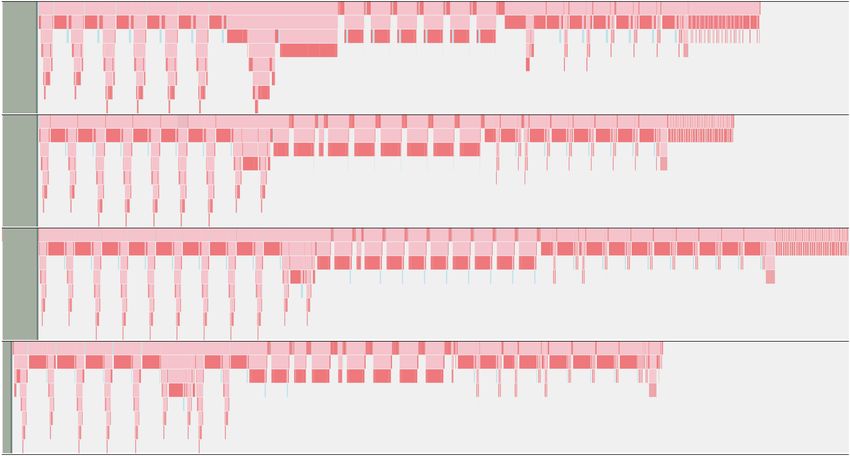
Under review as a conference paper at ICLR 2021

Model Parallelism: Model Parallelism is used when a model is too large to fit in the memory of
a single device and is instead spread over multiple processors (Krizhevsky et al., 2012; Shazeer
et al., 2018; Harlap et al., 2018; Lepikhin et al., 2020). This is increasingly common as state of
the art performance continues to improve with increasing model size (Brown et al., 2020). Model
parallelism unfortunately has a few downsides: (i) High communication costs – the total training
time for larger networks can become dominated by communication costs (Simonyan & Zisserman,
2015), which in the worst case can grow quadratically with the number of devices, and can reach up
to 85% of the total training time of a large model such as VGG-16 (Harlap et al., 2018; Simonyan
& Zisserman, 2015); (ii) Device under-utilization – forward propagation and backward propagation
are both synchronous operations, which can result in processor under-utilization in model-parallel
systems. This problem becomes worse as we increase the number of layers (Ben-Nun & Hoefler,
2018; Jia et al., 2014; Collobert et al., 2011; Abadi et al., 2016; Huang et al., 2018).
Pipeline Parallelism: Due to the forward and backward locking, using multiple devices to process
consecutive blocks of the deep model would make an inefficient use of the hardware resources.
Pipelining (Harlap et al., 2018) concurrently passes multiple mini-batches to multiple layers on
multiple devices. This increases device utilization but can introduce staleness and consistency issues
which lead to unstable training. Harlap et al. (2018) alleviates the consistency issue by storing past
versions of each layer. Huang et al. (2019) addresses the staleness issue by pipelining microbatches
and synchronously updating at the end of each minibatch. Guan et al. (2019) builds on this work
by introducing a weight prediction strategy and Yang et al. (2020) investigates to what extent the
tradeoff between staleness/consistency and device utilization is necessary. Local updates on the
other hand can keep device utilization high with both small and large batches and avoid the weight
staleness problem.
Local Learning Rules: Local learning describes a family of methods that perform parameter up-
dates based only on local information, where locality is defined as dependence of neighboring neu-
rons, layers, or groups of layers. The earliest local method we are aware of is Hebbian Learning
(Hebb, 1949) which has further been explored in BCM theory (Izhikevich & Desai, 2003; Co-
esmans et al., 2004), Oja’s rule (Oja, 1982), Generalized Hebbian Learning (Sanger, 1989), and
meta-learned local learning rules (Bengio et al., 1990; 1992; Metz et al., 2018; Gu et al., 2019). Ar-
chitectures like Hopfield Networks (Hopfield, 1982) and Boltzmann Machines (Ackley et al., 1985)
also employ a local update, and predate backprogation in deep learning. Modern variants of local
training methods have attempted to bridge the performance gap with backpropagation. These in-
clude projection methods such as Hebbian learning rules for deep networks (Krotov & Hopfield,
2019; Grinberg et al., 2019; Ryali et al., 2020), and local layer-wise learning with auxiliary losses
(Belilovsky et al., 2019a;b). Most similar to our work is decoupled greedy layer-wise learning
(Belilovsky et al., 2019b; Löwe et al., 2019), which trained auxiliary image classifiers greedily, and
local contrastive learning (Xiong et al., 2020). These methods mainly focus on matching the perfor-
mance of backpropagation with respect to training epochs, whereas our work focuses on tradeoffs.
Finally, while not local in the sense that parallelized layers still optimize for the global objective,
Huo et al. (2018b) parallelize layers by caching gradients and using delayed gradient signals to
overcome the backward locking problem and update decoupled layers in parallel.

3   L OCAL PARALLELISM

Given a deep neural network, we divide the layers into a sequence of J blocks, which may contain
one or more layers. Each block is trained independently with an auxiliary objective, and receives the
activations output by the previous block as input or, in the case of the first block, the data from the
sampled minibatch. We consider five variants to train this sequence of J blocks: backpropagation,
greedy local parallelism, overlapping local parallelism, and chunked local parallelism, as shown in
Figure 2. We also include a baseline method of just training the last, or last two, layers. In all of the
local methods, training occurs by attaching objective functions to the end of each block and back
propagating the signal locally into the corresponding block or blocks. In this work the auxiliary
objective functions that we use take the same form as the global objective. For example, to train
a classifier on CIFAR-10, we attach auxiliary linear classifiers to each local block. See Belilovsky
et al. (2019b) for further discussion on the form of this objective.

                                                   3
Under review as a conference paper at ICLR 2021
Layer 1
Layer 2
Loss
Loss Loss Loss Loss
Layer 3
(a) Backpropagation (b) Greedy
Layer 4
Forward
Loss Loss Loss Loss Loss Backward
(c) Overlapping (d) Chunked
Figure 2: A comparison forward progagation and backward propagation patterns for the architec-
tures considered in this work – (a) backpropagation, (b) greedy local updates, (c) overlapping local
updates, and (d) chunked local updates.
Backpropagation: In our notation, backpropagation groups all layers into one block and thus J = 1.
The parameters are updated with one instance of global error correction. While backpropagation
ensures that all weights are updated according to the final output loss, it also suffers from forward and
backward locking (Jaderberg et al., 2017), an issue that local parallelized methods aim to resolve.
Greedy local parallelism: A straightforward approach to enable local training is to attach an auxil-
iary network to each local layer, which generates predictions from the activations of hidden layers.
After generating predictions, each local gradient is backpropagated to its respective local block,
shown in Figure 2(b). The activations are then passed as input to the next layer. We refer to this
approach, introduced in (Belilovsky et al., 2019b), as greedy. Greedy local parallelism is the most
parallelizable of all the schemes we consider. However, a potential downside is that fully greedy
updates force the layers to learn features that are only relevant to their local objective and preclude
inter-layer communication, which may result in lower evaluation performance for the global objec-
tive, or worse generalization.
Overlapping local parallelism: One issue with the purely greedy approach is that features learned
for any individual block may not be useful for subsequent blocks, since there is no inter-block prop-
agation of gradient. For this reason, we consider overlapping local architectures where the first layer
of each block is also the last layer of the previous block, as shown in Figure 2(c), though overlapping
of more layers is also possible. This redundancy enables inter-block propagation of gradient that is
still local, since only neighboring blocks overlap. However, this comes at the cost of running ad-
ditional backward passes. The overlapping architecture has appeared before in Xiong et al. (2020),
but was used only for contrastive losses. Ours is the first work to investigate overlapping local archi-
tectures for standard prediction objectives in computer vision and language. Overlapping updates
are parallelizable, but come with the additional complexity of keeping duplicates of the overlapping
components and averaging updates for these layers.
Chunked local parallelism: The greedy architecture is maximally parallel in the sense that it dis-
tributes one layer per block. However, it is also possible to have fewer parallel blocks by combining
multiple layers into one. We refer to this architecture, shown in Figure 2(d), as chunked local par-
allelism. This method trades off parallelizability and therefore throughput for an error signal that
propagates through more consecutive layers. It differs from overlapping local parallelism by not
needing to duplicate any layer. While previous work has investigated the asymptotic performance
of chunked parallelism (Belilovsky et al., 2019b), ours is the first to consider the compute effi-
ciency and parallelizability of local parallelism. By stacking multiple layers per each parallelized
block, chunked parallelism sits between fully parallelized methods, such as greedy and overlapping
updates, and fully sequential methods like backpropagation.
4 E FFICIENT T RAINING ON PARETO F RONTIERS
We explore the trade off between total computational cost and the amount of wallclock time needed
to train a particular machine learning model to a target performance, similar to the analysis in Mc-
4Under review as a conference paper at ICLR 2021
Cuttoff loss: 1.000000 Cuttoff loss: 0.100000 Cuttoff loss: 0.010000 Cuttoff loss: 0.001000
101 101 101 101
Backprop
Greedy
Cost (total PFlops) Overlapping
Two Chunk Greedy
100 100 100 100 Three Chunk Greedy
Last Layer
Last 2 Layers
10 1 10 1 10 1 10 1
10 5 10 4 10 3 10 2 10 5 10 4 10 3 10 2 10 5 10 4 10 3 10 2 10 5 10 4 10 3 10 2
Walltime (sequential PFlops) Walltime (sequential PFlops) Walltime (sequential PFlops) Walltime (sequential PFlops)
Figure 3: Pareto optimal curves showing the cost vs time tradeoff for an 8-layer, 4096 unit MLP
trained on CIFAR-10 reaching a particular cutoff in training loss. We find that under no circumstance
is backprop the most efficient method for training. ‘×’ symbol denotes trained models.
Candlish et al. (2018). We use floating point operations (FLOPs) as our unit of both cost and time,
as they do not couple us to a particular choice of hardware. Cost is proportional to the total FLOPs
used. We report time as the number of sequential FLOPs needed assuming we can run each example,
and in the case of the local methods, each layer, in parallel. We refer the reader to Appendix A for
detailed information on how total and sequential FLOPs are computed for each experiment.
We compare how backpropagation scales with compute across a variety of local methods: (i) greedy
(Figure 2(b)), (ii) overlapping (Figure 2(c)), (iii) two and three chunk greedy (Figure 2(d)), where
we split the network into two or three pieces that are trained in a greedy fashion, (iv) last layer & last
two layers, a simple baseline where we only backpropagate through the last one or two layers and
keep the rest of the network parameters fixed. We apply these methods on a variety of architectures
and data including a dense feed-forward network, a ResNet50 network (He et al., 2016) trained
on ImageNet (Russakovsky et al., 2015), and a Transformer (Vaswani et al., 2017) model trained
on LM1B (Chelba et al., 2013). In Appendix C, we provide results for additional feed-forward
networks, a ResNet18 trained on ImageNet, and a larger Transformer, as well as further architecture
details. For each model and training method, we perform a large sweep over batch size as well as
other optimization hyperparameters, and only display the best-performing runs on the Pareto optimal
frontier. See Appendix B for more detail.
The resulting figures all follow the same general structure. Models train with low total cost when
the amount of available compute is large. By increasing batch size, the amount of compute utilized
per parallel process can be reduced efficiently until a critical batch size is reached, at which point
further increasing the batch size results in diminishing returns in terms of compute efficiency, which
is similar to results reported for backpropagation in (McCandlish et al., 2018). We find that, in
most cases, local updates significantly increase the training speed over deep networks in the high-
compute regime, and therefore utilize less total compute than backpropagation. When applicable, we
additionally show tables of the best achieved results across all parameters ignoring the time to reach
these values. In this setting, we find that backpropagation usually achieves the best performance.
This is partially due to the fact that all of these models are trained for a fixed number of examples,
and partially due to the fact that backpropagation makes higher use of the capacity of a given model,
which we further investigate in Section 5.
4.1 S YNTHETIC : MLP’ S OVER - FITTING TO CIFAR-10
As a proof of concept we first demonstrate optimization performance on an eight layer MLP with
4096 hidden units, performing classification on the CIFAR-10 dataset (Krizhevsky et al., 2009).
Hyperparameter and optimization details can be found in Appendix B.1. From the resulting Pareto
frontiers shown in Figure 3, we find that in no circumstance is backpropagation the best method to
use. In the high compute regime, we find that local methods enable training up to 10× faster (e.g.
in 0.001 cutoff).
4.2 L ANGUAGE M ODELING : T RANSFORMERS ON LM1B
Next we explore a small (6M parameter) Transformer (Vaswani et al., 2017) trained on
LM1B (Chelba et al., 2013). We build off of an implementation in Flax Developers (2020). Hyperpa-
rameters and optimization details can be found in Appendix B.2. We find that, for the higher cutoffs,
many of the local methods vastly outperform backpropagation. For the lower cuttofs (≤ 4.0), we
5Under review as a conference paper at ICLR 2021
102
Cuttoff loss: 5.000000 102
Cuttoff loss: 4.000000 102
Cuttoff loss: 3.900000 102
Cuttoff loss: 3.800000
Backprop
Greedy
101 101 101 101
Cost (total PFlops) Overlapping
Two Chunk Greedy
100 100 100 100 Three Chunk Greedy
Last Layer
Last 2 Layers
10 1 10 1 10 1 10 1
10 2 10 2 10 2 10 2
10 6 10 5 10 4 10 3 10 2 10 6 10 5 10 4 10 3 10 2 10 6 10 5 10 4 10 3 10 2 10 6 10 5 10 4 10 3 10 2
Walltime (sequential PFlops) Walltime (sequential PFlops) Walltime (sequential PFlops) Walltime (sequential PFlops)
Backprop Overlapping Greedy 2 Chunk Greedy 3 Chunk Greedy Last Layer Last 2 Layers
3.623 3.662 3.757 3.734 3.758 4.635 4.230
Figure 4: Total compute cost vs. serial compute cost (walltime) Pareto curves computed from
validation loss for a 6M parameter parameter transformer. We find that for high loss cutoffs (e.g.
5.), significant speedups (around 4×) can be obtained. For cutoffs of 4.0, and 3.9 speedups (around
2×) are still possible, but only with the overlapping method. For even lower cut offs, 3.8, we find the
majority of our models are unable to obtain this loss. In the bottom table we show the best achieved
validation loss for each training method maximized across all hyperparameters.
find that while backpropagation is more efficient in the high-time regime, local methods train sig-
nificantly faster in the high-compute regime, and can train 2× faster than backpropagation. These
local methods do not reach as low of a minimum in the given training time however. See Figure 4.
4.3 I MAGE C LASSIFICATION : R ES N ET 50 ON I MAGE N ET
Next we explore performance of optimization parallelism on a ResNet50 model trained on the Ima-
geNet dataset (Russakovsky et al., 2015) (Figure 5). Hyperparameter and configuration details can
be found in Appendix C.1. We find, as before, that for many cutoff values local parallelism shows
gains over backpropagation in the high-compute regime. However, at the cutoff of 74% these gains
shrink and the local methods are slightly less efficient. We hypothesize this is in-part due to in-
creased overfitting by the local methods. To see this we can observe that local methods are much
more competitive when evaluated on training accuracy. This suggests that given more data these
local methods will be competitive.
5 P ROBING B EHAVIOR OF L OCAL U PDATES
In the previous section we showed that in some cases local parallelism can provide large speedups
over backpropagation but suffers in terms of the best achievable performance. In this section we
explore why and how these methods work, and discuss limitations.
Gradient Angles: Local parallelism does not follow the gradient of the underlying function. Instead
it computes a local, greedy approximation. To check the quality of this approximation we measure
the angle between the true gradient, and the gradient computed with our greedy method (Figure 6a).
We find positive angles which imply that these directions are still descent directions. As one moves
further away from the end of the network these similarities shrink.
Larger Block Sizes Improve Generalization: As noted in Huo et al. (2018a;b) and Belilovsky
et al. (2019b), using chunked local parallelism with more parallel blocks can decrease performance.
Here we show that practically this reduction in performance seems to stem mainly from a worsening
generalization gap, with train and test results shown for various chunk sizes in Figure 6. A chunk
size of nine is simply backprop, and a chunksize of one is fully greedy.
Capacity: Ability to Fit Random Labels: Throughout our work we find that models trained with
local updates don’t make as efficient use of model capacity. This is not necessarily a problem,
but represents a tradeoff. Researchers have found that increased model sizes can be used to train
faster without leveraging the extra capacity to its fullest (Raffel et al., 2019; Kaplan et al., 2020).
Additionally, techniques like distillation can be used to reduce model size (Hinton et al., 2015).
We demonstrate this capacity issue by fitting random labels with a ResNet on CIFAR-10, shown in
Figure 6.
6Under review as a conference paper at ICLR 2021
103
Cuttoff valid acc: 50% 103
Cuttoff valid acc: 60% 103
Cuttoff valid acc: 70% 103
Cuttoff valid acc: 74%
Backprop
Greedy
102 102 102 102
Cost (total PFlops) Overlapping
Two Chunk Greedy
101 101 101 101 Three Chunk Greedy
Last Layer
100 100 100 100 Last 2 Layers
10 1 10 1 10 1 10 1
10 5 10 3 10 1 10 5 10 3 10 1 10 5 10 3 10 1 10 5 10 3 10 1
Walltime (sequential PFlops) Walltime (sequential PFlops) Walltime (sequential PFlops) Walltime (sequential PFlops)
103
Cuttoff train acc: 50% 103
Cuttoff train acc: 60% 103
Cuttoff train acc: 70% 103
Cuttoff train acc: 74%
Backprop
Greedy
102 102 102 102
Cost (total PFlops)
Overlapping
Two Chunk Greedy
101 101 101 101 Three Chunk Greedy
Last Layer
100 100 100 100 Last 2 Layers
10 1 10 1 10 1 10 1
10 5 10 3 10 1 10 5 10 3 10 1 10 5 10 3 10 1 10 5 10 3 10 1
Walltime (sequential PFlops) Walltime (sequential PFlops) Walltime (sequential PFlops) Walltime (sequential PFlops)
Backprop Overlapping Greedy 2 Chunk Greedy 3 Chunk Greedy Last Layer Last 2 Layers
Valid 0.775 0.679 0.633 0.772 0.745 0.272 0.421
Train 0.841 0.695 0.628 0.821 0.790 0.247 0.401
Figure 5: Total compute cost vs walltime frontier for ResNet50 models trained on ImageNet. We
show the cost/time to reach a certain cutoff measured on validation accuracy (top) and training accu-
racy (bottom). With low cutoffs (50%, 60%, 70%), modest speedups can be obtained on validation
performance. With higher cutoffs (74%) however backprop is optimal. In the subsequent table, we
show the best accuracies reached for each method across all configurations. We find that the least
parallelized method, Two Chunk Greedy, is the only local method competitive with backprop on
validation accuracy.
(a) Gradient similarity (b) Multi-chunk performance (c) Fitting to random labels
1.00 0.8
100 99 99 99 99 99 Backprop
Cosine Similarity
98
Train Accuracy
0.75 0.6 Local
95
Accuracy
0.50 91 91 91
90
0.25 90 89
88 0.4
0.00 85 Train
Layer: Test 0.2
0.25 1st 2nd 3rd 4th 5th (last)
80
0 2000 4000 6000 8000 10000 nine five four three two one 0 20 40 60 80 100
Iterations Epoch Layers per parallel chunk
Figure 6: Properties and trade-offs of local parallelism. (a) The cosine similarity between backprop-
agation gradients and greedy local gradients for a 5 layer convolutional neural network. Gradients
in the last two layers are identical to, or converge towards, those from backpropagation. Earlier
layer local gradients are increasingly dissimilar to those from backpropagation but are still descent
directions. (b) An ablation of the number of layers per chunk for ResNet18 trained on CIFAR-10.
Adding more layers per chunk improves generalization, while the training loss is roughly equal
across different chunk sizes. (c) Backprop and greedy local training is performed on a ResNet18,
trained on CIFAR-10 with random labels. Global backpropagation demonstrates higher capacity, in
that it is able to memorize the dataset better than local greedy backpropagation.
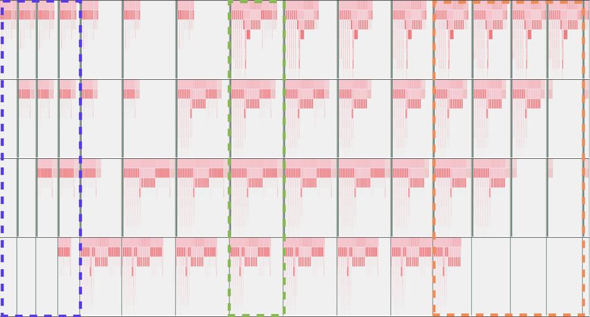
Local Methods Learn Different Features: One way to show differences between local and non-
local methods is to look at the features learned. For each method we test we take the best performing
model and visualize the first layer features. The results are shown in Figure 7. Qualitatively, we see
similar first layer features from Backprop and Two/Three Chunk local parallelism. The more greedy
approaches (Overlap, Greedy) yield a different set of features with fewer edge detectors. Finally,
when training with only the last layers, the input layer is not updated, and the features are random.
7Under review as a conference paper at ICLR 2021
Backprop Two Chunk Three Chunk Overlap Greedy Last 2
Figure 7: First layer filters taken at the end of training normalized by the min and max value per filter.
We find the more global methods (Backprop, Two Chunk, Three Chunk) learn similar distributions
over features. However more greedy approaches (Overlap and Greedy) learn visually distinct, less
edge-like, features. Finally the Last 2 filters are random, because the input layer is never updated.
6 R EALIZED P ERFORMANCE G AINS
Here we show that performance gains of local parallelism can be realized on real hardware, and
that they are similar to or better than pipelined backpropagation despite the increased computation
needed for auxiliary losses. We train ResNet34, ResNet50 and ResNet101 (He et al., 2016) on
the ImageNet dataset (Deng et al., 2009), and compare throughput (images per second) between
chunked local parallelism and synchronous pipelined backpropagation (Huang et al., 2019). We
implement the models in TensorFlow (Abadi et al., 2016) and train them across 4 or 8 Intelligence
Processing Units (IPUs – see details in Appendix E). Note that neither local nor pipeline config-
urations make use of data parallelism which could be applied identically in both cases. We use
activation recomputation in the case of pipelined backprop (see discussion in Appendix D.3). The
results in Table 1 show that chunked local parallelism can achieve similar or greater throughput
compared to pipelined backpropagation, for the same local batch size. This provides evidence
that local parallelism can enable similar hardware efficiency without necessitating an increase of
minibatch size. It is therefore amenable to a greater level of data parallelism before performance
degradation due to a large global batch size. The difference in throughput between backpropagation
and local parallelism with the same local batch size is primarily due to the poor utilisation during
the “ramp-up” and “ramp-down” phases of the pipelined backpropagation. This can be mitigated by
running the pipeline in the steady state for more stages (compare rows 4 and 5 of Table 1). However,
this results in the accumulation of gradients from a larger number of local batches, thus costing a
larger effective batch size. With greedy local parallelism, updates can be applied asynchronously
and the pipeline can be run in steady state indefinitely, after an initial ramp-up phase. Hardware
utilization analysis and further discussion can be found in Appendix D.
Network Local batch size Backprop batch size # IPUs Speedup over backprop
32 32 × 8 4 8%
ResNet34
32 32 × 16 8 37%
16 16 × 8 4 28%
ResNet50 16 16 × 16 8 32%
16 16 × 32 8 12%
4 4 × 16 8 33%
ResNet101
8 8 × 16 8 41%
Table 1: Increase in throughput for ImageNet training with chunked local updates vs pipelined back-
prop. Backprop batch size a × b, where a is the microbatch size and b is the number of microbatches
over which gradients are accumulated.
7 C ONCLUSION
In this work we demonstrated that local parallelism is a competitive alternative to backpropagation in
the high-compute training regime, and explored design decisions and trade-offs inherent in training
with local parallelism. We summarize some main takeaways from our work:
8Under review as a conference paper at ICLR 2021
• Speed vs. Performance: Greedy local parallelism should be used if speed and compute-
efficiency are the primary objectives. Chunked local parallelism should be used if perfor-
mance is the primary objective.
• Gains in High-Compute Regime: Local parallelism can be useful to prolong compute-
efficient scaling, and therefore faster training, with larger batch sizes once data parallelism
begins to saturate.
• Comprehensive Analysis: Local parallelism can be applied across multiple modalities (vi-
sion, language) and architectures (MLPs, ResNets, Transformers).
We hope that local methods will enable new research into large models. By lowering communication
requirements – particularly latency requirements surrounding synchronization – we believe that local
parallelism can be used to scale up and train more massive models in a more distributed fashion.
R EFERENCES
Martin Abadi, Paul Barham, Jianmin Chen, Zhifeng Chen, Andy Davis, Jeffrey Dean, Matthieu
Devin, Sanjay Ghemawat, Geoffrey Irving, Michael Isard, Manjunath Kudlur, Josh Levenberg,
Rajat Monga, Sherry Moore, Derek G. Murray, Benoit Steiner, Paul Tucker, Vijay Vasudevan,
Pete Warden, Martin Wicke, Yuan Yu, and Xiaoqiang Zheng. TensorFlow: A system for large-
scale machine learning. In 12th USENIX Symposium on Operating Systems Design and Imple-
mentation (OSDI 16), pp. 265–283, 2016.
David H. Ackley, Geoffrey E. Hinton, and Terrence J. Sejnowski. A learning algorithm for Boltz-
mann machines. Cognitive Science, 9(1):147–169, 1985.
Eugene Belilovsky, Michael Eickenberg, and Edouard Oyallon. Greedy layerwise learning can scale
to ImageNet. In 36th International Conference on Machine Learning, pp. 583–593, 2019a.
Eugene Belilovsky, Michael Eickenberg, and Edouard Oyallon. Decoupled greedy learning of
CNNs. arXiv preprint arXiv:1901.08164 [cs.LG], 2019b.
Tal Ben-Nun and Torsten Hoefler. Demystifying parallel and distributed deep learning: An in-depth
concurrency analysis. arXiv preprint arXiv:1802.09941 [cs.LG], 2018.
Samy Bengio, Yoshua Bengio, Jocelyn Cloutier, and Jan Gecsei. On the optimization of a synap-
tic learning rule. In Preprints Conf. Optimality in Artificial and Biological Neural Networks,
volume 2. Univ. of Texas, 1992.
Yoshua Bengio, Samy Bengio, and Jocelyn Cloutier. Learning a Synaptic Learning Rule. University
of Montreal, 1990.
Christopher Berner, Greg Brockman, Brooke Chan, Vicki Cheung, Przemysław Debiak, Christy
Dennison, David Farhi, Quirin Fischer, Shariq Hashme, Chris Hesse, et al. Dota 2 with large
scale deep reinforcement learning. arXiv preprint arXiv:1912.06680, 2019.
Tom B. Brown, Benjamin Mann, Nick Ryder, Melanie Subbiah, Jared Kaplan, Prafulla Dhari-
wal, Arvind Neelakantan, Pranav Shyam, Girish Sastry, Amanda Askell, Sandhini Agarwal,
Ariel Herbert-Voss, Gretchen Krueger, Tom Henighan, Rewon Child, Aditya Ramesh, Daniel M.
Ziegler, Jeffrey Wu, Clemens Winter, Christopher Hesse, Mark Chen, Eric Sigler, Mateusz Litwin,
Scott Gray, Benjamin Chess, Jack Clark, Christopher Berner, Sam McCandlish, Alec Radford,
Ilya Sutskever, and Dario Amodei. Language models are few-shot learners. arXiv preprint
arXiv:2005.14165 [cs.CL], 2020.
Ciprian Chelba, Tomas Mikolov, Mike Schuster, Qi Ge, Thorsten Brants, Phillipp Koehn, and Tony
Robinson. One billion word benchmark for measuring progress in statistical language modeling.
arXiv preprint arXiv:1312.3005, 2013.
Jianmin Chen, Xinghao Pan, Rajat Monga, Samy Bengio, and Rafal Jozefowicz. Revisiting dis-
tributed synchronous SGD. arXiv preprint arXiv:1604.00981 [cs.LG], 2016.
9Under review as a conference paper at ICLR 2021
Tianqi Chen, Mu Li, Yutian Li, Min Lin, Naiyan Wang, Minjie Wang, Tianjun Xiao, Bing Xu,
Chiyuan Zhang, and Zheng Zhang. Mxnet: A flexible and efficient machine learning library for
heterogeneous distributed systems. arXiv preprint arXiv:1512.01274, 2015.
Ting Chen, Simon Kornblith, Mohammad Norouzi, and Geoffrey Hinton. A simple framework for
contrastive learning of visual representations. arXiv preprint arXiv:2002.05709 [cs.LG], 2020.
Michiel Coesmans, John T. Weber, Chris I. De Zeeuw, and Christian Hansel. Bidirectional parallel
fiber plasticity in the cerebellum under climbing fiber control. Neuron, 44(4):691–700, 2004.
Ronan Collobert, Koray Kavukcuoglu, and Clement Farabet. Torch7: A matlab-like environment
for machine learning. In BigLearn, NIPS 2011 Workshop, 2011.
Dipankar Das, Sasikanth Avancha, Dheevatsa Mudigere, Karthikeyan Vaidynathan, Srinivas Srid-
haran, Dhiraj Kalamkar, Bharat Kaul, and Pradeep Dubey. Distributed deep learning using syn-
chronous stochastic gradient descent. arXiv preprint arXiv:1602.06709 [cs.DC], 2016.
Jeffrey Dean, Greg Corrado, Rajat Monga, Kai Chen, Matthieu Devin, Mark Mao, Marc aurelio
Ranzato, Andrew Senior, Paul Tucker, Ke Yang, Quoc V. Le, and Andrew Y. Ng. Large scale
distributed deep networks. In Advances in Neural Information Processing Systems 25 (NIPS
2012), pp. 1223–1231, 2012a.
Jeffrey Dean, Greg Corrado, Rajat Monga, Kai Chen, Matthieu Devin, Mark Mao, Marc’aurelio
Ranzato, Andrew Senior, Paul Tucker, Ke Yang, et al. Large scale distributed deep networks. In
Advances in neural information processing systems, pp. 1223–1231, 2012b.
J. Deng, W. Dong, R. Socher, L.-J. Li, K. Li, and L. Fei-Fei. ImageNet: A large-scale hierarchical
image database. In IEEE Conference on Computer Vision and Pattern Recognition (CVPR 2009),
pp. 248–255, 2009.
Li Deng, Dong Yu, and John Platt. Scalable stacking and learning for building deep architectures.
In IEEE International Conference on Acoustics, Speech and Signal Processing (ICASSP 2012),
pp. 2133–2136, 2012.
Flax Developers. Flax: A neural network library for JAX designed for flexibility, 2020. URL
https://github.com/google-research/flax/tree/prerelease.
Priya Goyal, Piotr Dollár, Ross Girshick, Pieter Noordhuis, Lukasz Wesolowski, Aapo Kyrola, An-
drew Tulloch, Yangqing Jia, and Kaiming He. Accurate, large minibatch SGD: Training ImageNet
in 1 hour. arXiv preprint arXiv:1706.02677 [cs.CV], 2017.
Leopold Grinberg, John J. Hopfield, and Dmitry Krotov. Local unsupervised learning for image
analysis. arXiv preprint arXiv:1908.08993 [cs.CV], 2019.
Keren Gu, Sam Greydanus, Luke Metz, Niru Maheswaranathan, and Jascha Sohl-Dickstein. Meta-
learning biologically plausible semi-supervised update rules. bioRxiv, 2019.
Lei Guan, Wotao Yin, Dongsheng Li, and Xicheng Lu. Xpipe: Efficient pipeline model parallelism
for multi-gpu dnn training, 2019.
Aaron Harlap, Deepak Narayanan, Amar Phanishayee, Vivek Seshadri, Nikhil Devanur, Greg
Ganger, and Phil Gibbons. PipeDream: Fast and efficient pipeline parallel DNN training. arXiv
preprint arXiv:1806.03377 [cs.DC], 2018.
Kaiming He, Xiangyu Zhang, Shaoqing Ren, and Jian Sun. Deep residual learning for image recog-
nition. In IEEE Conference on Computer Vision and Pattern Recognition (CVPR 2016), pp.
770–778, 2016.
Donald O. Hebb. The organization of behavior; a neuropsychological theory. Wiley, 1949.
Olivier J Hénaff, Aravind Srinivas, Jeffrey De Fauw, Ali Razavi, Carl Doersch, SM Eslami, and
Aaron van den Oord. Data-efficient image recognition with contrastive predictive coding. arXiv
preprint arXiv:1905.09272, 2019.
10Under review as a conference paper at ICLR 2021
Tom Hennigan, Trevor Cai, Tamara Norman, and Igor Babuschkin. Haiku: Sonnet for JAX, 2020.
URL http://github.com/deepmind/dm-haiku.
Geoffrey Hinton, Oriol Vinyals, and Jeff Dean. Distilling the knowledge in a neural network. arXiv
preprint arXiv:1503.02531 [stat.ML], 2015.
John J. Hopfield. Neural networks and physical systems with emergent collective computational
abilities. Proceedings of the National Academy of Sciences, 79(8):2554–2558, 1982.
Yanping Huang, Youlong Cheng, Ankur Bapna, Orhan Firat, Mia Xu Chen, Dehao Chen, Hy-
oukJoong Lee, Jiquan Ngiam, Quoc V. Le, Yonghui Wu, and Zhifeng Chen. GPipe: Easy scaling
with micro-batch pipeline parallelism. arXiv preprint arXiv:1811.06965 [cs.CV], 2018.
Yanping Huang, Youlong Cheng, Ankur Bapna, Orhan Firat, Dehao Chen, Mia Chen, HyoukJoong
Lee, Jiquan Ngiam, Quoc V Le, Yonghui Wu, et al. Gpipe: Efficient training of giant neural
networks using pipeline parallelism. In Advances in neural information processing systems, pp.
103–112, 2019.
Raphael Hunger. Floating Point Operations in Matrix-vector Calculus. Munich University of Tech-
nology, Inst. for Circuit Theory and Signal, 2005.
Zhouyuan Huo, Bin Gu, and Heng Huang. Training neural networks using features replay. In
Advances in Neural Information Processing Systems 31 (NeurIPS 2018), pp. 6659–6668, 2018a.
Zhouyuan Huo, Bin Gu, Qian Yang, and Heng Huang. Decoupled parallel backpropagation with
convergence guarantee. arXiv preprint arXiv:1804.10574 [cs.LG], 2018b.
Sergey Ioffe and Christian Szegedy. Batch normalization: Accelerating deep network training by
reducing internal covariate shift. In Francis Bach and David Blei (eds.), Proceedings of the 32nd
International Conference on Machine Learning, volume 37 of Proceedings of Machine Learning
Research, pp. 448–456, Lille, France, 07–09 Jul 2015. PMLR. URL http://proceedings.
mlr.press/v37/ioffe15.html.
Eugene M. Izhikevich and Niraj S. Desai. Relating STDP to BCM. Neural Computation, 15(7):
1511–1523, 2003.
Max Jaderberg, Wojciech Marian Czarnecki, Simon Osindero, Oriol Vinyals, Alex Graves, David
Silver, and Koray Kavukcuoglu. Decoupled neural interfaces using synthetic gradients. In 34th
International Conference on Machine Learning, pp. 1627–1635, 2017.
Yangqing Jia, Evan Shelhamer, Jeff Donahue, Sergey Karayev, Jonathan Long, Ross Girshick, Ser-
gio Guadarrama, and Trevor Darrell. Caffe: Convolutional architecture for fast feature embed-
ding. arXiv preprint arXiv:1408.5093 [cs.CV], 2014.
Zhe Jia, Blake Tillman, Marco Maggioni, and Daniele Paolo Scarpazza. Dissecting the graphcore
ipu architecture via microbenchmarking, 2019.
Jared Kaplan, Sam McCandlish, Tom Henighan, Tom B Brown, Benjamin Chess, Rewon Child,
Scott Gray, Alec Radford, Jeffrey Wu, and Dario Amodei. Scaling laws for neural language
models. arXiv preprint arXiv:2001.08361 [cs.LG], 2020.
Alex Krizhevsky, Vinod Nair, and Geoffrey Hinton. CIFAR-10 and CIFAR-100 datasets. URl:
https://www. cs. toronto. edu/kriz/cifar. html, 6, 2009.
Alex Krizhevsky, Ilya Sutskever, and Geoffrey E. Hinton. ImageNet classification with deep convo-
lutional neural networks. In Advances in Neural Information Processing Systems 25 (NIPS 2012),
pp. 1097–1105, 2012.
Dmitry Krotov and John J. Hopfield. Unsupervised learning by competing hidden units. Proceedings
of the National Academy of Sciences, 116(16):7723–7731, 2019.
Dmitry Lepikhin, HyoukJoong Lee, Yuanzhong Xu, Dehao Chen, Orhan Firat, Yanping Huang,
Maxim Krikun, Noam Shazeer, and Zhifeng Chen. Gshard: Scaling giant models with conditional
computation and automatic sharding. arXiv preprint arXiv:2006.16668, 2020.
11Under review as a conference paper at ICLR 2021
Sindy Löwe, Peter O’Connor, and Bastiaan Veeling. Putting an end to end-to-end: Gradient-isolated
learning of representations. In Advances in Neural Information Processing Systems 32 (NeurIPS
2019), pp. 3039–3051, 2019.
Dominic Masters and Carlo Luschi. Revisiting small batch training for deep neural networks. arXiv
preprint arXiv:1804.07612, 2018.
Sam McCandlish, Jared Kaplan, Dario Amodei, and OpenAI Dota Team. An empirical model of
large-batch training. arXiv preprint arXiv:1812.06162 [cs.LG], 2018.
Luke Metz, Niru Maheswaranathan, Brian Cheung, and Jascha Sohl-Dickstein. Meta-learning up-
date rules for unsupervised representation learning. In International Conference on Learning
Representations, 2018.
Luke Metz, Niru Maheswaranathan, Jeremy Nixon, Daniel Freeman, and Jascha Sohl-Dickstein.
Understanding and correcting pathologies in the training of learned optimizers. In International
Conference on Machine Learning, pp. 4556–4565, 2019.
Luke Metz, Niru Maheswaranathan, Ruoxi Sun, C Daniel Freeman, Ben Poole, and Jascha Sohl-
Dickstein. Using a thousand optimization tasks to learn hyperparameter search strategies. arXiv
preprint arXiv:2002.11887, 2020.
Feng Niu, Benjamin Recht, Christopher Re, and Stephen J. Wright. Hogwild!: A lock-free approach
to parallelizing stochastic gradient descent. arXiv preprint arXiv:1106.5730 [math.OC], 2011.
Erkki Oja. Simplified neuron model as a principal component analyzer. Journal of Mathematical
Biology, 15(3):267–273, 1982.
Alexander Ororbia, Ankur Mali, C Lee Giles, and Daniel Kifer. Continual learning of recurrent
neural networks by locally aligning distributed representations. IEEE Transactions on Neural
Networks and Learning Systems, 2020.
Alain Petrowski, Gerard Dreyfus, and Claude Girault. Performance analysis of a pipelined back-
propagation parallel algorithm. IEEE Transactions on Neural Networks, 4(6):970–981, 1993.
Alec Radford, Jeffrey Wu, Rewon Child, David Luan, Dario Amodei, and Ilya Sutskever. Language
models are unsupervised multitask learners. 2019. OpenAI Blog.
Colin Raffel, Noam Shazeer, Adam Roberts, Katherine Lee, Sharan Narang, Michael Matena, Yanqi
Zhou, Wei Li, and Peter J Liu. Exploring the limits of transfer learning with a unified text-to-text
transformer. arXiv preprint arXiv:1910.10683 [cs.LG], 2019.
David E Rumelhart, Geoffrey E Hinton, and Ronald J Williams. Learning internal representations
by error propagation. Technical report, California Univ San Diego La Jolla Inst for Cognitive
Science, 1985.
Olga Russakovsky, Jia Deng, Hao Su, Jonathan Krause, Sanjeev Satheesh, Sean Ma, Zhiheng
Huang, Andrej Karpathy, Aditya Khosla, Michael Bernstein, Alexander C. Berg, and Li Fei-Fei.
ImageNet Large Scale Visual Recognition Challenge. International Journal of Computer Vision
(IJCV), 115(3):211–252, 2015. doi: 10.1007/s11263-015-0816-y.
Chaitanya K. Ryali, John J. Hopfield, Leopold Grinberg, and Dmitry Krotov. Bio-inspired hashing
for unsupervised similarity search. arXiv preprint arXiv:2001.04907 [cs.LG], 2020.
Terence D. Sanger. Optimal unsupervised learning in a single-layer linear feedforward neural net-
work. Neural Networks, 2(6):459–473, 1989.
John Schulman, Nicolas Heess, Theophane Weber, and Pieter Abbeel. Gradient estimation using
stochastic computation graphs. In Advances in Neural Information Processing Systems, pp. 3528–
3536, 2015.
Alexander Sergeev and Mike Del Balso. Horovod: fast and easy distributed deep learning in Ten-
sorFlow. arXiv preprint arXiv:1802.05799, 2018.
12Under review as a conference paper at ICLR 2021
Christopher J. Shallue, Jaehoon Lee, Joseph Antognini, Jascha Sohl-Dickstein, Roy Frostig, and
George E. Dahl. Measuring the effects of data parallelism on neural network training. arXiv
preprint arXiv:1811.03600 [cs.LG], 2018.
Noam Shazeer, Youlong Cheng, Niki Parmar, Dustin Tran, Ashish Vaswani, Penporn Koanantakool,
Peter Hawkins, HyoukJoong Lee, Mingsheng Hong, Cliff Young, et al. Mesh-tensorflow: Deep
learning for supercomputers. In Advances in Neural Information Processing Systems, pp. 10414–
10423, 2018.
David Silver, Julian Schrittwieser, Karen Simonyan, Ioannis Antonoglou, Aja Huang, Arthur Guez,
Thomas Hubert, Lucas Baker, Matthew Lai, Adrian Bolton, et al. Mastering the game of go
without human knowledge. nature, 550(7676):354–359, 2017.
Karen Simonyan and Andrew Zisserman. Very deep convolutional networks for large-scale image
recognition. In International Conference on Learning Representations, 2015.
Ashish Vaswani, Noam Shazeer, Niki Parmar, Jakob Uszkoreit, Llion Jones, Aidan N. Gomez,
Łukasz Kaiser, and Illia Polosukhin. Attention is all you need. In Advances in Neural Infor-
mation Processing Systems 31 (NIPS 2017), pp. 5998–6008, 2017.
Oriol Vinyals, Igor Babuschkin, Junyoung Chung, Michael Mathieu, Max Jaderberg, Wojciech M
Czarnecki, Andrew Dudzik, Aja Huang, Petko Georgiev, Richard Powell, et al. Alphastar: Mas-
tering the real-time strategy game starcraft ii. DeepMind blog, pp. 2, 2019.
Yuwen Xiong, Mengye Ren, and Raquel Urtasun. LoCo: Local contrastive representation learning.
arXiv preprint arXiv:2008.01342 [cs.LG], 2020.
Bowen Yang, Jian Zhang, Jonathan Li, Christopher Ré, Christopher R. Aberger, and Christopher De
Sa. Pipemare: Asynchronous pipeline parallel dnn training, 2020.
Xiru Zhang, Michael Mckenna, Jill P. Mesirov, and David L. Waltz. An efficient implementation
of the back-propagation algorithm on the connection machine CM-2. In Advances in Neural
Information Processing Systems 2 (NIPS 1989), pp. 801–809, 1989.
13Under review as a conference paper at ICLR 2021
A C ALCULATION OF T OTAL FLOP S AND S EQUENTIAL FLOP S
To construct the Pareto curves used in this work we need some estimate of compute time. Obtaining
hardware independent measurements of compute cost and compute time is desirable, but in general
impossible, as different hardware makes different trade offs for compute efficiency. In this work
we choose to use a theoretical estimate of compute costs based on floating point operation (FLOP)
counting. In all three models, we divide the costs up into three measurements: FLOPs needed for
a forward pass through a layer, flops needed for the auxiliary loss computation, and a multiplier to
compute the number of flops for a backward pass. For simplicity, we average the compute costs
across layers. While this is strictly not feasible in reality with a batch size of one per device, we can
come close to approximating it by using more or less parallel hardware per layer. This is relatively
simple to implement given the minimal communication overhead. We additionally take into account
optimizer flops, which we we approximate as ten times the number of parameters, but this results
negligible.
A.1 C ALCULATIONS PER M ODEL
MLP: An MLP is parameterized by the hidden size, N , and the number of layers, L. The first
layer’s total flops are from matrix vector multiplication, a bias add of size N , and a ReLU (which
we assume costs 1 FLOP per entry). This yields a total size of (2 ∗ I ∗ N − I) + N + 2 ∗ N
FLOPs, where I is the input size (Hunger, 2005). The auxiliary classifiers consist of a matrix vector
multiplication to size 10, a bias add, and a softmax cross entropy loss. We assume the softmax costs
5 flops per estimate leading to a flop estimate of (2 ∗ N ∗ 10 − N ) + 10 + 5 ∗ 10. For this problem,
we approximate the backward multiplier to be 1.5. For the MLP model used in the main text (with
hidden size N = 4096 and L = 8 layers), the average forward cost per layer is 32514176.0 flops,
and the auxiliary loss 77884.0 flops.
For the remaining models, we compute our estimates of these components by first us-
ing JAX to convert our models to TensorFlow functions, and then leveraging TensorFlow’s
tf.compat.v1.profiler.profiler.
ResNet50: This model has L = 17 layers and contains 38711720 parameters. We find that the
average forward flop count per example, per layer is 5479411.176470588, the auxiliary loss per
layer is 3382457.3529411764, and the backward multiplier is 2.0280375672996596.
ResNet18: This model has L = 9 layers, and has 13170792 parameters. We find that the average
forward flop count per example, per layer is 1640544.352941176, the auxiliary loss flop count per
example per layer is 565900.6470588235, and the backward multiplier is 2.08565879129763.
Transformer small: This model has L = 4 layers. We find that the average forward cost per
example, per layer is 13837446.0, the auxiliary loss is 1163904.0, and the backward multiplier is
1.6581083035860107.
Transformer large: This model has L = 6 layers. We find that the average forward cost per
example, per layer is 51037318.0, the auxiliary cost is 4653696.0, and the backward multiplier is
1.7526391044859857.
A.2 C ALCULATIONS PER M ETHOD
In all cases, we first obtain the total computation cost in terms of flops and then compute time (or
sequential flops) by dividing by the max amount of parallelism (assuming that each example and
each layer are run concurrently). As stated before, this is not strictly possible to implement in hard-
ware. In reality, however, we expect more than one example to be used per device in combination
with data parallelism and thus appropriate load balancing can be done.
All of these calculations are a function of the 4 numbers described above (forward cost, auxiliary
cost, backward multiplier and the optimizer cost) in addition to batch size and the number of gradi-
ents steps until the target loss is reached.
Backprop: Per step, backprop involves running one forward pass and one backward pass of the
entire network plus plus one auxiliary head for the last layer loss computation. The cost per example
14Under review as a conference paper at ICLR 2021
is computed as follows:
cost per example = (1 + backward multiplier) ∗ (forward cost ∗ layers + aux cost)
cost = cost per step example ∗ steps ∗ batch size + steps ∗ optimizer cost
time = cost/batch size
Greedy: Per step, the greedy method requires running one forward and backward pass for L layers
and L auxilary loss computations.
cost per example = (1 + backward multiplier) ∗ ((forward cost + aux cost) ∗ layers)
cost = cost per step example ∗ steps ∗ batch size + steps ∗ optimizer cost
time = cost/(batch size ∗ layers)
Overlapping: Because we are using overlapping chunks of layers, additional compute must be
performed. This method uses one full forward pass though the entire network plus two backward
passes for each non terminal layer. The terminal layer only requires one less layer of computation.
We additionally need one forward and backward pass of each auxiliary loss. An additional average
of gradients is required which incurs extra compute per layer.
cost per example =(forward cost + aux cost) ∗ layers+
(layers − 1) ∗ backward multiplier ∗ (2 ∗ forward cost + aux cost)+
backward multiplier ∗ (forward cost + aux cost)
cost =cost per step example ∗ steps ∗ batch size + steps ∗ (optimizer cost + 2 ∗ parameters)
time =cost/(batch size ∗ layers)
Two/Three chunk: In this, we perform a full forward + backward pass for each layer plus two or
three auxiliary losses. Lets call the number of chunks K for the equations bellow.
cost per example = (1 + backward multiplier)(forward cost + K ∗ aux cost)
cost = cost per step example ∗ steps ∗ batch size + steps ∗ optimizer cost
time = cost/(batch size ∗ K)
Last One/Two Layers: These methods require a full forward pass, a single auxilary loss computa-
tion and then a backward pass on the last K layers. To calculate time, we assume this last K layers
is the smallest atomic chunk that can be run and we divide up the remaining layers accordingly.
cost per example = (layers ∗ forward costaux cost) + backward multiplier ∗ (K ∗ forward cost + aux cost)
cost = cost per step example ∗ steps ∗ batch size + steps ∗ optimizer cost
num parallel = (layers + K ∗ backward mult)/(K ∗ (1 + backward mult))
time = cost/(batch size ∗ num parallel)
15Under review as a conference paper at ICLR 2021
B H YPERPARAMETER AND C ONFIGURATION D ETAILS FOR E XPERIMENTAL
R ESULTS
B.1 MLP ON CIFAR-10
We sweep the batch size from 64-524,288 in powers of 2. At each batch size, we train models using
learning rate tuned Adam (with six values log spaced between 1e-4 and 3e-2) as well as the first
50 optimizers taken from opt list to provide a stronger baseline (Metz et al., 2020). All models are
trained for three million examples on an eight core TPU-V2 using gradient accumulation to control
memory usage. We select a sequence of cut off values (the loss for which we attempt to reach in the
shortest time) and plot the Pareto frontier of the different training methodology in Figure 3.
B.2 T RANSFORMERS ON LM1B
Our Transformer has 4 layers, 8 heads per attention layer, 128-dimensional query, key, and value
vectors, 256-dimensional hidden layers, and 128-dimensional embeddings. We train on length 128
sequences formed from subword tokenization with a vocabulary size of 8k. Each Transformer layer
is treated as a separate parallelizable component. Our auxiliary classifiers consist of layer norm and
a linear projection back to the vocabulary, with a softmax cross entropy loss. We sweep batch sizes
in powers of two from 32 to 524,288. At each batch-size we either train Adam with six different
learning rates taken evenly spaced on a log scale between 1e-4 and 3e-2 and the first 50 optimizers
from opt list (Metz et al., 2020). All models are run until they have processed 50 million sequences,
an an 8-core TPU-V2 with gradient accumulation to control memory. We chose four cutoff values
computed on validation loss to show early in training (a value of 5.0 and 4.0), the value chosen by
Shallue et al. (2018) (3.9), and a loss value slightly lower (3.8). Results can be found in Figure 4.
C A DDITIONAL PARETO C URVES E XPERIMENTS
We provide additional Pareto curves for different architecture models.
C.1 R ES N ETS ON I MAGE N ET
We build our code off of the Haiku implementation (Hennigan et al., 2020). We break the network up
by putting the first convolution, and each residual block into a separate parallelizable component For
auxiliary losses we apply batch normalization (Ioffe & Szegedy, 2015), then ReLU, then compute
mean across the spatial dimensions, and finally perform a linear projection to the output classes.
We sweep batch sizes from 8 to 524,288 in powers of 2. For each batch size we randomly sample
optimizer hyperparameters for both the SGDM optimizer with a staircase schedule described in
Goyal et al. (2017) and from the first 50 configurations in opt list. The resulting cost wall time
Pareto curves for both validation accuracy and training accuracy are shown in Figure 5.
C.2 MLP S
We provide MLP’s trained matching Section 4.1 but using a different number of hidden units. In
addition to 4096 units, we show 1024, 256, and 64 units in Figure 8. We find the last 2 layers
performs well for larger networks, as there is enough capacity, but is considerably less useful as
model size shrinks.
C.3 T RANSFORMER L ARGE
In this section we explore a larger transformer than that in Section 4.2. This transformer matches
the default settings of of (Flax Developers, 2020). It has has 6 layers, 8 heads per attention layer,
512-dimensional query, key, and value vectors, 512-dimensional hidden layers, and 512-dimensional
embeddings. We train on length 128 sequences formed from subword tokenization with a vocab size
of 32k. We show results in Figure 9. Unlike in the small transformer and due to increased compute
costs, we random sample configurations instead of running all of them.
16You can also read