Dynamic Interaction between Shared Autonomous Vehicles and Public Transit: A Competitive Perspective
←
→
Page content transcription
If your browser does not render page correctly, please read the page content below
Dynamic Interaction between Shared Autonomous Vehicles and Public
                                                                       Transit: A Competitive Perspective

                                                                    Baichuan Moa , Zhejing Caob , Hongmou Zhangc,d , Yu Shene , Jinhua Zhaoc,∗
                                                     a Department of Civil and Environmental Engineering, Massachusetts Institute of Technology, Cambridge,    MA 02139
                                                                             b School of Architecture, Tsinghua University, Beijing, China 100084
                                                         c Department of Urban Studies and Planning, Massachusetts Institute of Technology, Cambridge, MA      02139
                                                        d Future Urban Mobility IRG, Singapore–MIT Alliance for Research and Technology Centre, Singapore      138602
                                                 e Key Laboratory of Road and Traffic Engineering of the Ministry of Education, Tongji University, Shanghai,   China 201804
arXiv:2001.03197v2 [physics.soc-ph] 3 Feb 2020

                                                 Abstract
                                                 The emerging autonomous vehicles (av) can either supplement the public transportation (pt) system or
                                                 be a competitor with it. This paper focuses on this competition in a hypothetical scenario—“if both av
                                                 and pt operators are profit-oriented,” and uses an agent-based model to quantitatively evaluate the system
                                                 performance in this competition from the perspectives of four stakeholders—av service operator, pt operator,
                                                 passengers, and public authority. In our model, av operator updates its supply by changing fleet sizes while
                                                 pt by adjusting headways, and both use heuristic approaches to update supply in order to increase profits.
                                                 We implement the model in the first-mile scenario in Tampines, Singapore. In four regulation scenarios—
                                                 two by two combinations regarding whether av and pt are allowed to change supplies—we find that since
                                                 av can release the bus operator from low-demand routes, the competition can lead to higher profits of
                                                 both, and higher system efficiency, simultaneously, rather than a one-sided loss-gain result. For pt, after
                                                 supply updates, spatially the services are concentrated to short feeder routes directly to the subway station,
                                                 and temporally concentrated to peak hours. For passengers, the competition reduces their travel time but
                                                 increases their travel costs. Nonetheless, the generalized travel cost is still reduced when counting the value
                                                 of time. For system efficiency and sustainability, bus supply adjustment can increase the bus average load
                                                 and reduce total passenger car equivalent (PCE), while the av supply adjustment shows the opposite effect.
                                                 For policy implications, the paper suggests that pt should be allowed to optimize its supply strategies under
                                                 specific operation goals constraints, and av operation should be regulated to relieve its externality on the
                                                 system, including limiting the number of licenses, operation time, and service areas, which makes av operated
                                                 like a complementary mode to pt. Besides, compensation/price incentives may be targeted passengers who
                                                 suffer from higher travel costs and longer travel time due to av and pt supply adjustment.
                                                 Keywords: shared mobility-on-demand system; autonomous vehicles; public transportation; agent-based
                                                 simulation; market Competition

                                                 1. Introduction

                                                 The emergence of autonomous vehicles (av) as a new transportation mode is anticipated to extensively
                                                 influence the future urban transportation system in different aspects, including traffic flow stability and
                                                 throughput rates (Talebpour and Mahmassani, 2016), network congestion levels (Fagnant and Kockelman,
                                                 2015), land use patterns (Koh and Wich, 2012), and road safety (Zhang et al., 2016). As a critical component
                                                 of urban transportation, public transportation (pt) systems cannot avoid the impact of av. Due to the
                                                 uncertainty of how the av system may evolve, many possible scenarios of av–pt interaction have been
                                                 proposed (Lazarus et al., 2018). Some researchers argue that avs will be competitors to the pt systems
                                                 (Levin and Boyles, 2015; Chen and Kockelman, 2016) or even replace them (Mendes et al., 2017), while
                                                 some are optimistic to the av–pt integration, stating that they could be complementary (Lu et al., 2017).

                                                   ∗ Corresponding author
                                                     Email address: jinhua@mit.edu (Jinhua Zhao)

                                                 Preprint submitted to Elsevier                                                                           February 4, 2020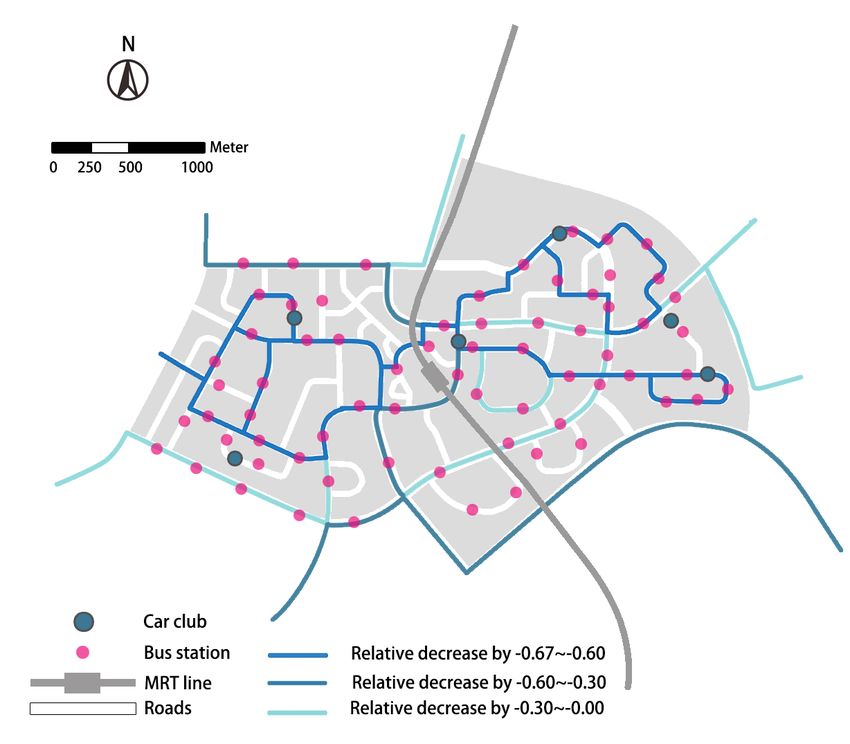
Av–pt integration has been widely studied under various operation and regulation scenarios. For exam-
ple, Salazar et al. (2018) proposed a tolling scheme for an av–pt intermodal system, which shows significant
reduction of travel time, costs, and emissions compared to an av-only scenario. Wen et al. (2018) designed a
transit-oriented autonomous mobility-on-demand (amod) system, revealing the trade-off between level of ser-
vice and operation cost. They found encouraging ride-sharing, allowing in-advance requests, and combining
fare with transit help to stimulate sustainable travel.
    Conversely, for av–pt competition, a comprehensive analysis is still lacking. Most prior research only
evaluated the effect of av based on aggregate models, but did not specify the competition mechanisms
between av and pt (Levin and Boyles, 2015; Childress et al., 2015). Recently, agent-based models (ABM)
have been used to investigate the av–pt competition. For example, both Liu et al. (2017) and Mendes et al.
(2017) argued that traditional pt services may not survive once the shared av services become available.
Nonetheless, prior research using ABM all considered the av–pt interaction to be static or a single-shot
game—how pt systems will evolve when av is introduced—rather than a repeated game with av and pt
competing by adjusting supplies.
    This paper aims to extend the ABM approach to simulate the repeated games between av and pt, and
to evaluate the performance of both systems, such as level of service, operators’ financial viability, and
transport efficiency. We assume that both av and pt can be profit-oriented competitors with dynamic
adjustable supply strategies under certain policy constraints.
    Competition per se is neither good or bad. In classic economics, in ideal situation market competition can
lead to optimal resource allocation. However, due to the possibility of market failure, regulations are often
imposed on competition, or even mandate certain cooperation. In this paper, we envision four regulation
scenarios, corresponding to four regulation levels, as listed in Table 1.
    The four scenarios are differentiated by the regulations of the supplies of pt and av—either be fixed
or adjustable. A “fixed” scenario is one in which the operators of either av or pt are NOT allowed to
change their supply. An “adjustable” scenario is one in which operators can adjust their supply based on
profit-oriented strategies. An overview of the four scenarios is given below.
   • The “status quo” scenario corresponds to a fully-regulated transportation market without competition
     (Shen et al., 2018). The fare structure, route network, service areas are all set by transport author-
     ities. The operators in this scenario are only responsible for the operation, management, and fleet
     maintenance.
   • The “av-only” scenario corresponds to TNC-regulated organization structure (Shen et al., 2018), where
     the av operation can be licensed or regulated by public authorities, while the services are still provided
     by the private operators and operated independent from transit agencies (e.g., in New York City,
     London, and Singapore).
   • The “pt-only” scenario corresponds to the “Scandinavian” organization structure (Costa, 1996; van de
     Velde, 1999), where the transport authority sets service goals and then contracts out transit services
     to private operators. Pt operators make operational decisions to maximize their profits while ensuring
     service standards.

   • The “av–pt” scenario is close to the U.K.-deregulation structure (Wilson, 1991), where pt and av
     operators are profit-oriented competitors but both are also regulated by the public authority.

                                Table 1: Regulation scenarios assumed in this paper

                                                                    PT supply
                                     Scenarios
                                                               Fixed     Adjustable
                                              Fixed          Status quo   Pt-only
                             AV supply
                                            Adjustable        Av-only      Av–pt

    According to Lesh (2013), the first/last mile connection to subway station shows the highest potential for
market competition between av and pt. Thus, we select the first-mile trip market in Tampines, Singapore
as a focus area, with only buses comprising of the pt system.

                                                         2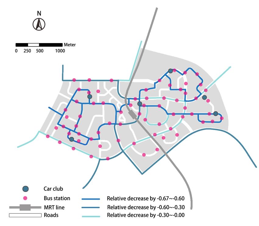
As for operation strategies, for simplicity of discussion, we assume av can only adjust the fleet size and
pt can only adjust the headway. Service fare and bus routes typically are regulated by governments, and
thus are assumed fixed throughout the paper.
    We evaluate the av–pt competition system from the perspectives of 1) av and pt operators, based on their
financial viability, 2) passengers, based on the level of service of both systems, and 3) transport authority,
based on efficiency and sustainability. The details of performance metrics are given in later sections.
    The contributions of this paper are twofold. First, the paper for the first time in literature simulates
the dynamic reciprocal supply strategies between profit-oriented av and pt systems; Second, we analyze the
impact of four different regulation scenarios on the competition;
    This paper is organized as follows. Section 2 presents a literature review and identifies the research gaps.
Section 3 presents the specification of the ABM used in this paper. Section 3.3 explains the performance
metrics in this paper. Section 4 discusses the results, and Section 5 concludes the paper.

2. Literature Review

Av is expected to reshape the future transportation system from different perspectives. Many advantages
of av, such as absolute compliance, expanded service hours, reduced labor forces and human errors make it
an efficient mode of urban transportation, which enables the reduction of operation cost and serves travel
demand smaller fewer fleet sizes (Fernández L. et al., 2008; Alonso-Mora et al., 2017; Spieser et al., 2014).
    Given the promising application of av, many recent studies have examined the impact of av in different
aspects, such as traffic flows (Talebpour and Mahmassani, 2016), road congestion (Fagnant et al., 2015),
land use (Koh and Wich, 2012), and road safety (Zhang et al., 2016). Talebpour and Mahmassani (2016)
used a micro-simulation model to evaluate the impact of connected and autonomous vehicles on traffic flows,
which showed that av can improve string stability and help to prevent shockwave formation and propagation.
Azevedo et al. (2016) applied an integrated agent-based micro-simulation model to design and evaluate the
impact of av on people’s travel behavior. They found that the new av technology can change people’s
travel patterns, specifically in terms of mode shares, route choices and activity destinations. Fagnant and
Kockelman (2014) found that each shared av can replace around 11 conventional vehicles, but adds up to
10% more travel distance than comparable non-shared av trips. There are also empirical studies in Lisbon
(Martinez and Viegas, 2017), Toronto (Kloostra and Roorda, 2019) and New Jersey (Zhu and Kornhauser,
2017), which reveals av technology can reduce travelled vehicle kilometres and emissions (Martinez and
Viegas, 2017), decrease average travel time (Kloostra and Roorda, 2019), and reduce the number of vehicles
on roads (Martinez and Viegas, 2017).
    However, despite the large volume of recent research the impact of av, research focusing on the av–pt
interaction is still lacking. Two major relationships between av and pt have been discussed in the literature.
    First, av and pt can be complementary and integrated. Av and pt can be cooperative in a way that
av is integrated as a part of pt system for social welfare. In line with this assumption, Ruch et al. (2018)
used a simulation model to analyze whether av can substitute the rural pt lines. It was shown that such
a service can operate at a lower cost and with a higher service level when the pt lines are short and are
underutilized. Similarly, Shen et al. (2018) designed an av–pt integration system with amod as an alternative
to low-demand bus routes, which showed that the integrated system has the potential of enhancing service
quality, occupying fewer road resources and being financially sustainable. Another cooperative scenario is
the multi-modality between av and pt. For example, Yap et al. (2016) conducted a stated preference survey
to analyze the use of automated vehicles as egress of train trips. They found that av is a good alternative
to the first-class train passengers. Liang et al. (2016) used an integer programming model to study av
as a last-mile connection to train trips, which showed that using automated taxis can reduce the pick-up
cost and improve profit. Vakayil et al. (2017) proposed a hybrid transit system where amod serves as the
first- and last-mile feeder for the subway. The results show that an integrated system can provide up to a
50% reduction in total vehicle miles traveled. These studies provide sufficient analysis toward the av–pt
integration relationship. Also, the co-operation strategies for av and pt are also designed (Salazar et al.,
2018).
    Second, av can be competitive with traditional pt when av is operated privately, and competes for market
shares and profit. The analysis of this scenario is very limited. Based on a multiclass four-step model, Levin
and Boyles (2015) found that the transit ridership will decrease when av is introduced. Similarly, Childress

                                                       3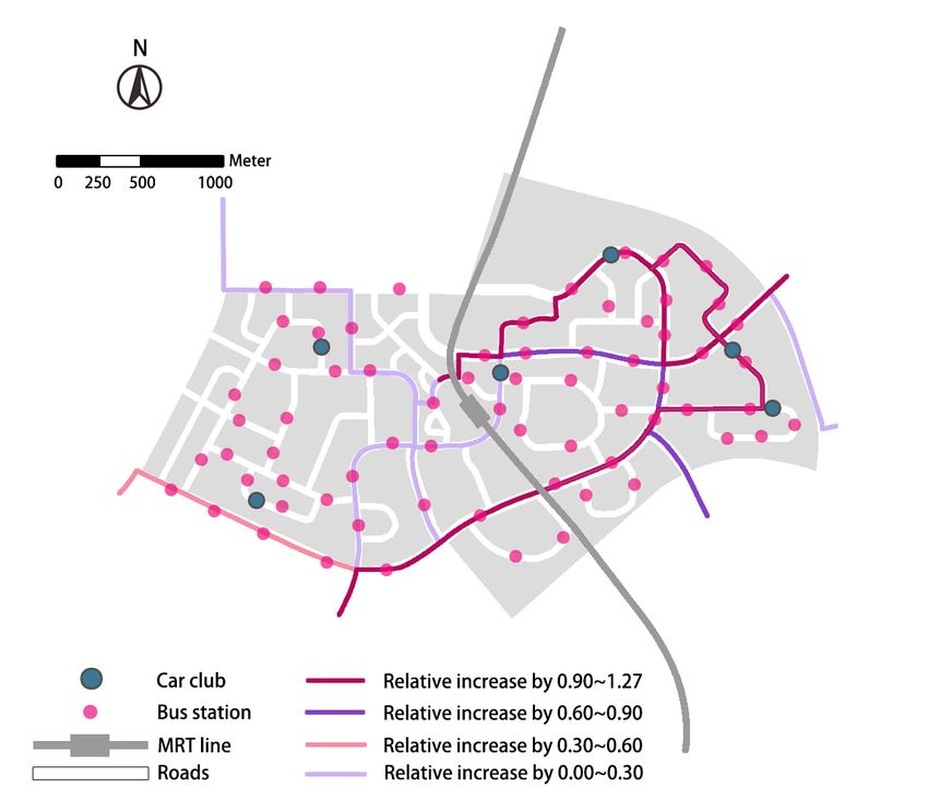
et al. (2015) used an activity-based model to evaluate the impact of av, which revealed a reduction of
pt’s mode share. Liu et al. (2017) simulated the impact of shared av based on the case study of Austin,
Texas, with results showing that conventional pt services may not survive once the shared av services become
available. Mendes et al. (2017) developed an event-based simulation model to compare the shared av services
with the proposed light rail services in New York City, which found that av is more cost-efficient in providing
the same level of service. Basu et al. (2018) applied an activity-driven agent-based simulation approach to
test the impact of av on mass transit and found that amod indirectly acts as a replacement to mass transit.
    Understanding how av competes with pt is critical for managing future pt services and developing
sound intervention on the private transportation market. However, the existing studies addressing av–pt
competition focused on the static interaction process, i.e., only looking at what will happen when av is
introduced as a one-shot game. However, as competitors, it is highly likely that av and pt will dynamically
adjust the operation strategies in the market as repeated games. These interactive dynamics have not been
considered in the literature. Moreover, most existing studies only evaluate the av’s impact on the mode
share of pt, without a comprehensive assessment of the cost and benefit of different stakeholders in the
system, including operators, passengers, and transport authorities.
    In this paper, we use an agent-based model to simulate the competition between av and pt as a repetitive
game, with both parties trying to increase their profits. We also comprehensively evaluate the system from
different stakeholders’ perspectives, including the financial conditions, level of services, sustainability and
transport efficiency, which aims to fill the research gap in the literature.

3. System Design

We use the Tampines Planning Area in Singapore as the study area to illustrate our av–pt competition
model, and the focus on the first-mile trips heading to the Tampines Mass Rapid Transit (MRT) station
from surrounding residential blocks.
    In Singapore, walking and buses are currently the dominant modes for first-mile trips (Mo et al., 2018).
Bus service in Singapore is highly regulated by the Land Transport Authority (LTA), which is responsible
for its fare structure and route design. The LTA contracts out bus services to different bus operators on a
five-year basis.

3.1. Basic Assumptions
Based on the characteristics and operational structures of the Singapore transport system, we make the
following assumptions for the av–pt competition model.
 (a) System level
        • Travel mode: Before av entering the market, walking, bus and ride-hailing are the only travel
          modes available for the first-mile trips. After av emerges, ride-hailing will be replaced by the
          amod. This assumption is corresponding to the Singapore autonomous vehicle initiative policies
          (Land Transport Authority, 2017).
        • Traffic condition: We focus on the mesoscopic simulation, the microscopic features such as road
          capacity, signal system, and driving behaviors are not considered in this study.
        • Demand and supply: The spatial and temporal distributions of travel demand are assumed to be
          fixed for all simulation days. The supply of av and pt can be adjusted for competition.
        • Information: The amod and pt’s supply information is complete and in real time for passengers’
          mode choice decisions.
 (b) Agent level

        • Ownership: Pt and amod are both operated by private enterprises, but under government regu-
          lation, i.e., they are in a constrained competition.
        • Objective: Pt and amod are able to adjust their supply to improve their profits.
        • Fare: Pt and amod’s fare structures are fixed by the government and cannot be changed.

                                                      4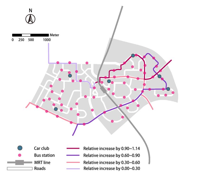
• Operation cost and subsidy: Pt and amod’s operation cost are proportional to their fleet size
and driving distance. There is no operation subsidy for pt based on the current Singapore policy
(Gopinath and Kuang, 2018).
• Constraints: Pt has a lower bound and an upper bound for the bus headway.
• Dynamic intraday supply: Amod and pt’s supply can be different in different time periods in a
day.
• Supply updating frequency: amod can update the next day’s supply strategy at the end of each
day. Pt can only update its supply strategy after a sufficiently long time (30 days in this paper;
more discussion in Section 3.5).
To summarize, amod updates supply daily by adjusting the vehicle fleet size in each time interval of the
next day, and pt adjusts its supply by changing the headway for each bus route in different time intervals
monthly.
Price adjustment is also a common practice to increase profit in market competition. However, to isolate
the impact of supply change, we only focus on supply in this paper, assuming prices to be fixed for both
pt and amod. Moreover, given the price regulation history of LTA, it is very likely that the amod will
be regulated on the fare structure to avoid price wars (Singapore Public Transport Council, 2019). Future
research can explore on a combined model incorporating supply change and pricing.
3.2. Study Area
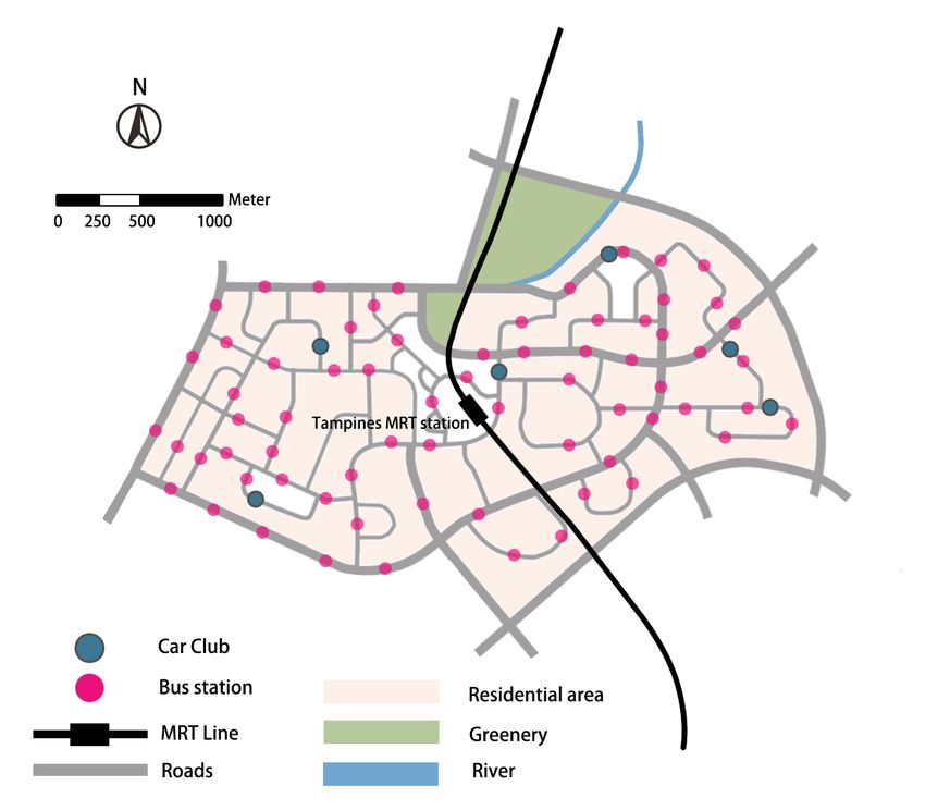
Tampines is a 6.86-km2 mixed residential and working area located in the east of Singapore (Figure 1). It is
centered around the Tampines MRT station, which is one of the busiest MRT stations in Singapore (Housing
& Development Board, 2015). 51 bus stops serve Tampines, with 26 bus routes connecting to the MRT
station. Three of them are dedicated feeder routes to the subway. The other 23 are passing-by routes. All 26
routes are included in the simulation model. We choose Tampines as a case to illustrate our model because
1) it possesses a significant first-mile demand to the MRT station, and 2) it embraces a large volume of bus
supply, which provides a non-trivial testbed for competition analysis.
Figure 1: Study Area
The first-mile travel demand is obtained from the transit smart card data. The dataset covers all pt trips
in August 2014. A normal workday in August 2014 is selected as the study date. Since the smart card data in
5Singapore includes both tap-ins and tap-outs, the accurate date and time of every entry and exit activity are
recorded, as well as the boarding and alighting stops/stations, which allows us to extract first-mile trips by
filtering the bus trips with a connecting subway trip. The temporal distribution of first-mile travel demand
in study day is shown in Figure 2. There are a total of 51,850 passengers entering the Tampines MRT station
during the study date.
Figure 2: Time-of-day Distribution of First-mile Demand to Tampines MRT Station
3.3. Stakeholders and System Evaluation
We evaluate the interests of multiple stakeholders in the av–pt competition. Table 2 identifies four key
stakeholders (passengers, amod operators, pt operators and transport authority) their evaluation indicators.
For passengers, the main interests are level-of-service and modal choice. The level-of-service indicators
include travel cost, total travel time, waiting time and generalized travel cost—calculated as the sum of
walking time, waiting time and riding time multiplied by the corresponding value of time (VOT). It is a
comprehensive value that incorporates both travel time and travel costs. The VOTs are derived from the
estimated choice model in Table B.1. In terms of modal choice, the number of travelers choosing walking,
bus and av are recorded, respectively.
For amod and pt operators, based on our profit-orientation assumption, their interests are financial
viability and supply. The financial viability indicators include operation cost, revenue, profit, and market
share, while the supply indicates the number of av/bus supplied.
For the transport authority, efficiency and sustainability are considered. The average load per vehicle is
one of the indicators for transport efficiency, which is calculated by total passenger travel distance divided
by total vehicle travel distance. As for sustainability, we consider the vehicle kilometers traveled (VKT) and
total passenger car equivalent (PCE). The unit PCE for a bus is set as 3.5 in this study (Ahuja, 2007).
These indicators are recorded in the simulation process, which shows the whole changing profile during
the competition between av and pt. The time of day distribution of some indicators is also recorded.
3.4. Agent Behaviors
The overall simulation system is composed of three main types of agents: buses, amod vehicles and passen-
gers. The pt system is derived from Shen et al. (2018)’s study, which has been calibrated and validated with
real-world data. Here we give an overview of the behaviors of the agents, with detailed formulation given in
Appendix A.
• Passengers’ mode choices are based on mixed logit models, and use trip-specific variables, including
waiting time, in-vehicle time, monetary cost, etc., and individual-specific variables, such as household
income; If a passenger chooses bus, we assume he/she walking to the closest bus stop; If there is no
bus available at the trip start time, and at the same time there is a shortage of amod, the agent walks
to the MRT station directly.
6Table 2: Evaluated Indicators of Stakeholders
Stakeholder Interests Indicators
Travel cost
Total travel time
Level of service
Waiting time
Passengers Generalized travel cost
Walking demand
Mode choice Bus demand
AV demand
Operation cost
Revenue
Financial viability
AMoD Operators Profit
Market share
Supply Average number of AV provided per hour
Operation cost
Revenue
Financial viability
PT Operators Profit
Market share
Supply Number of bus dispatched per day
AV average load per vehicle
Transport efficiency
Bus average load per vehicle
Transport Authority AV VKT
Sustainability Bus VKT
Total PCE (AV and PT)
• Amod dispatching is based on the first-come-first-serve principle upon passengers’ requests. The ve-
hicles follow the shortest paths from pick-up locations to the MRT station. When there is no empty
vehicle available, the dispatching center will then look for vehicles with passengers who agree to share
their trips. The amod operator updates the fleet size of each time period of a day, daily to increase its
profit.
• Buses follow existing routes given by the LTA. The operator for each bus route independently optimizes
its profit by changing the headway of each time period of a day, monthly.
3.5. Simulation Platform
We implemented the model on AnyLogic 8.1. The simulation is executed for T = 365 days to make sure that
the competition process converges. There are four sets of input variables/parameters: simulation setting
(0) (0)
parameters θ, initial supply strategies of bus SB , initial supply strategies of amod SA , and the first-mile
demand D. The detailed notations and values used are given in Table 3. The values of many constants are
chosen based on Singapore context, where details can be found in Appendix A.
The supply, profit, and supply changing unit are all time-specific for av, which means that for different
days and different time periods they may have different values. For buses, these variables are time- and
route-specific. The pseudo-code for simulation is shown in Algorithm 1.
As shown in Algorithm 1, the overall framework aims to simulate the interaction between av and pt
over time period T . One-Day-Sim is a pseudo function of running the simulation for a single day given the
supply, demand and θ, which can be seen as the engine of the simulation model. In this function, each agent
will follow the behaviors mentioned in Appendix A.
The profits of amod and pt can be obtained after running this function. The profit, supply and supply
change unit are then used as the input of function SupplyUpdate (shown in Algorithm 2), deriving the
updated supply strategies and new supply change unit for av and pt. It is worth noting that since we assume
the av supply updating frequency to be daily, this function is executed for av everyday, while for pt, this
function is executed every NB days considering the inflexibility of pt.
In reality, the schedule of pt should not be adjusted frequently considering peopleâĂŹs expectation for
its reliability. A reasonable changing frequency should be more than 6 months, which allows the transit
operator to notice the public, and gives people enough time to be prepared for the new schedule. However,
using NB =6 month will lead to a high computational load. Based on our numerical test, given a specific bus
schedule, the system will become stable in one or two weeks when only amod updates its supply. Thence,
7Table 3: Notations and Values of System Parameters
Categories Parameters/Variables Value
Duration of simulation (T ) 365 days
Supply changing unit reduced factor (γ) 0.5
Passenger choice lag factor (α) 0.5
Passenger mode choice parameters (β) See Table B.1
Passenger maximum av waiting time 10 min
Passenger maximum bus waiting time 30 min
Passenger ride-sharing-agreement rate 50%
Av supply time interval (iA ) 1 hour
Av supply updating frequency (NA ) 1 day
Simulation setting Av fixed operation cost 4 SGD/hour·veh
parameters (θ) Av variable operation cost 0.12 SGD/km
Av base distance of fare (db ) 1 km
Av base fare (fb ) 3.4 SGD
Av distance-based fare (f ) 0.22 SGD/400 m
Av detour discount rate of fare (λ) 2
L
Av supply lower bound (SA ) 0
U
Av supply upper bound (SA ) +∞
ini
Av initial supply changing unit (CA ) 10 vehicles
Bus supply time interval (iB ) 2 hour
Bus supply updating frequency (NB ) 30 days
Bus operation cost 2.71 SGD/km
Bus dwell time 30 sec
Bus fare 0.77 SGD/trip
U
Bus headway upper bound (SB ) 2100 sec
L
Bus headway lower bound (SB ) 210 sec
ini
Bus initial headway changing unit (CB ) 3 min
l,t,d
Bus headway of route l in time interval t on day d (SB ) Intermediate
Bus supply SB (d) l,t,d
Bus headway arrangement on day d (SB = [SB ]l,t ) Intermediate
(0)
Bus initial headway arrangement (SB ) See Appendix A.3
t,d
Number of av supplied in time interval t on day d (SA ) Intermediate
Av supply SA (d) t,d
Av supply strategies on day d (SA = [SA ]t ) Intermediate
(0)
Av initial supply strategies (SA ) See Appendix A.2
Demand D Demand of first-mile trips D See Figure 2
Amod profit in time interval t on day d (pt,d A ) Intermediate
(d)
Amod profit vector on day d (pA = [pt,d A ]t ) Intermediate
t,d
Av supply changing unit in time interval t for day d (CA ) Intermediate
Supporting (d) t,d
Av supply changing unit vector on day d (CA = [CA ]t ) Intermediate
variables
Bus profit of route l in time interval t on day d (pl,t,d B ) Intermediate
(d)
Bus profit vector day d (pB = [pl,t,d B ] l,t ) Intermediate
l,t,d
Bus headway changing unit of route l in time interval t for day d (CB ) Intermediate
(d) l,t,d
Bus headway changing unit vector on day d (CB = [CB ]l,t ) Intermediate
* Values “Intermediate” means the intermediate variables in the model.
8Algorithm 1 Agent-based Simulation
(0) (0)
1: procedure Simulation(θ, SB , SA , D)
(0) (0) (1) (0) (1) (0)
2: initialize pA = 0, pB = 0, SA = SA , SB = SB
(1) ini (1) ini
3: initialize CA = CA , CB = CB
4: let day counter d = 0
5: while d < T do
6: d=d+1
(d) (d) (d) (d)
7: pA , pB = One-Day-Sim(SB , SA , D | θ)
(d+1) (d+1) (d) (d−1) (d) (d)
8: SA , CA = SupplyUpdate(pA , pA , SA , CA )
9: if d mod NB == 0 then
(d+1) (d+1) (d) (d−NB ) (d) (d)
10: SB , CB = SupplyUpdate(pB , pB , SB , CB )
(d) ini
11: initialize CA = CA
12: else
(d+1) (d)
13: SB = SB
(d+1) (d)
14: CB = CB
15: return the system evaluation indicators (Table 2)
any value of NB that is greater than two weeks is equivalent to 6 months because the system state will not
change after 2 weeks. NB = 30 days is used in this study, which is able to simulate the long-period updating
frequency of the bus. The system evaluation indicators (Table 2) are recorded during the simulation process
and returned at the end of the model.
In terms of supply updating, we propose a heuristic algorithm, which applied to both amod and pt. Since
we have assumed that the spatial and temporal demand to be fixed, the profits across different time periods
and routes are independent. In other words, we assume people are not changing their departure times if
they observe fewer cars or buses in a time period, and profits then should be only functions of supply.
For example, pl,t,d
B , the profit of bus route l in time interval t on day d only depends on the headway
l,t,d
of route l in time interval t on day d. Then, we can adjust the supply of l in the same time period SB
to improve the corresponding profit as a single-variable optimization problem. Similarly for amod, if the
profit pt,d
A is greater than pA
t,d−1
, we know that the last change of supply CAt,d−1
led to the profit increase.
Thereupon, we can continue the increase of the fleet size of the same time period in the next day.
If the change of profits between two supply strategies becomes sufficiently small (in this paper we set the
threshold to be 5%), we reduce the size of changing unit by γ (i.e., C t,d+1 = γ · C t,d+1 ). This setting ensures
the convergence of results.
We acknowledge that the heuristic algorithm is a simplification for the profit maximization problem
because the profits of different time periods and routes are unlikely to be independent, especially when the
routes have overlapping stations. Nonetheless, we apply this simplified algorithm for the following reasons:
1) The concept of this algorithm is in line with the reality, where information is incomplete and every
adjustment is a trial of a new supply strategy based on previous experience; 2) Capturing the dependency
may lead to a complicated optimization problem, which is beyond the scope of this paper; 3) Based on the
numerical test, this heuristic algorithm can yield a continually improving profit. So it reaches the purpose
of mimicking agents’ competition for profit improvement, which is enough for this research.
4. Result Analysis
There is a rich space for all the value combinations of θ, as shown in Table 3. Each value combination
represents a distinct setting of competition markets —some are realistic and some are not. While it is not
the focus of this paper to systematically explore all possible scenarios, in this paper we only focus on four
specific combinations, labeled as four regulation scenarios introduced earlier (Table 1).
In the following subsections, we will show how the indicators of different stakeholders change during the
competition process.
9Algorithm 2 Supply Updating
1: procedure SupplyUpdate(p(d) , p(d−N ) , S (d) , C (d) )
2: let the index of elements in p(d) , p(d−N ) , S (d) and C (d) correspond with each other. (i.e., the
k element of p(d) , p(d−N ) , S (d) and C (d) represents the information of same time interval and same
th
route.)
3: initialize k = 0
4: while k < (length of p(d) ) do
5: k =k+1
6: let pk,d , pk,d−N , S k,d C k,d be the k th element in p(d) , p(d−N ) , S (d) and C (d) , respectively.
7: if pk,d > pk,d−N then
8: C k,d+1 = C k,d
9: else
10: C k,d+1 = −C k,d
k,d+1
11: S = S k,d + C k,d+1
k,d+1
12: if S violates the upper or lower bound constraints then
13: set S k,d+1 equal to the upper or lower bound
14: C k,d+1 = γ · C k,d+1
15: if the difference between pk,d and pk,d−N is small enough then:
16: C k,d+1 = γ · C k,d+1
(d+1)
17: let S = [S (k,d+1) ]k and C (d+1) = [C (k,d+1) ]k
(d+1)
18: return S , C (d+1)
4.1. PT Perspective
The revenue, operation cost and profit of the pt operator are shown in Figure 3. Each point represents the
average value of the corresponding month (same for all following graphs).
Since PT does not change supply in av-only and the status quo scenarios, the curves for these two
scenarios are relatively stable. The patterns for pt-only and av–pt scenarios are similar: the profit of PT
first increases and then stabilizes, which proves the effectiveness of the proposed supply updating algorithm.
(a) PT Revenue (b) PT Operation Cost (c) PT Profit
Figure 3: PT Finance over the Simulation Process
The final PT profit of the pt-only scenario is higher than those in all others’, which is intuitive because
there is no av competition in that scenario. The final PT profit of the av-only scenario is lower than that
in the status quo, which shows that the competition of av reduces the profit of pt.
Observing the revenue and operation cost of pt, we find that they both decrease over the simulation
period, where the operation cost shows a sharper reduction. This implies that the strategy for the bus in
the competition is to reduce the quantity of supply to reduce the operation cost.
In terms of bus supply and market share (Figure 4), we find the similar phenomenon. The number
of buses dispatched per day (i.e., bus supply) keeps decreasing and pt’s market share shows the similar
declining trend. Since bus will not change supply in pt-only and status quo scenarios, the supply curve for
10these two situations are flat lines. Comparing different scenarios, we find that bus will decrease to the lowest
service frequency with av’s competition. Correspondingly, the market share for av–pt scenario is also the
lowest.
(a) PT Supply (b) PT Market Share
Figure 4: PT Supply and Market Share over the Simulation Process
The operation cost of av–pt and pt-only scenarios are similar though their final supplies (Figure 4a) are
different. This is because most of the bus routes are not pure feeder routes and only crossing the study area.
These routes still need to serve the non-first-mile trips (see details in Appendix A.3), thus the corresponding
decrease of operation cost is very limited.
Another interesting phenomenon is that the additive effect of supply adjustment of both bus and av.
Take the bus market share as an example. The curve of pt-only scenario roughly represents how much
unprofitable market share is gradually “given up” by the pt operator. The av-only curve shows how much
market share the bus is grabbed by av (impact from av supply adjustment). The curve of av–pt scenario
thus shows the additive effect of two, which is nearly the sum of the above two reductions.
(a) PT Supply Temporal Distribution
(b) PT Supply Spatial Distribution
Figure 5: Distribution Change of PT Supply
11In addition to the total supply, we also zoom in to the change of temporal and spatial distributions of
supply before and after adjustment (Figure 5). Note that in the av-only and in the status quo scenarios bus
supplies are not adjustable, so they are not plotted. The bus supplies of the first month are the same for the
pt-only and the av–pt scenarios so only one curve of "initial" is shown.
From the temporal distribution, we found that after the supply adjustment, the numbers of dispatched
buses for most time periods except for the morning peak (6:00–10:00) are reduced. For the pt-only scenario,
the bus supply of the evening peak does not change, either. The implication is that the pt operator
concentrates supplies to morning peak and evening peak, which have larger demands and are more profitable.
As for spatial distribution, some routes (e.g., 29_1, 28_2) are allocated with higher frequencies, while
some routes (e.g., 291_2, 292_1) are adjusted to a lower service rate. The routes with increased and reduced
supplies are shown in Figure 6. Generally, the increased-supply routes are short and cost-efficient ones, which
cross the residential areas and go directly to the MRT station. The routes with decreased supply are long
and sinuous ones. Greater reduction in operation cost can be achieved by decreasing the supply of these
routes. Therefore, the spatial distribution change is related to an implicit coordination within the bus routes
(even if our algorithm does not consider the inter-routes coordination). To summarize, the pt operator will
reduce the supply for higher-cost routes, thus transfer the demand to the lower-cost routes, resulting in a
more profitable operation scheme.
(a) Routes with increased supply (AV–PT) (b) Routes with reduced suplly (AV–PT)
(c) Routes with increased supply (PT-only) (d) Routes with reduced supply (PT-only)
Figure 6: Spacial Distribution of PT Supply Change
124.2. AMoD Perspective
Figure 7 shows the amod revenue, operation cost and profit of amod over the simulation period. Since there
are big changes of amod’s supply in the first several days, the curves showing the supply of different days
in the first month are also shown with the red line, labeled on the upper x-axis. Note that the first-month
curve for the av-only and av–pt scenarios are the same because the bus supplies stay the same, and av does
not change in the other two scenarios. Therefore, only one curve is shown for the first month.
From the figures, we find that the amodâĂŹs revenue, operation cost and profit all increase rapidly at the
beginning, and then converge, which suggests that the amod operator will provide more services to improve
its profit in the competition. The trends of amod’s supply and market share also validate this point. As
shown in Figure 8, the amod’s supply and market share keep increasing during the first several months and
then become stable. The major change of amod’s supply from the status quo happened in the first month.
Comparing different scenarios, we find that the av–pt scenario can achieve the highest av profit and
the highest market share, though the av supply for this scenario is only the second-highest (av-only is the
highest), which implies that the bus supply adjustment can not only improve the profit of bus but also benefit
that of av. This is because the initial bus service is over-supplied for the first-mile market. When the bus
operator is allowed to adjust its supply, the yielded unprofitable travel demand is then served by av. This
observation corresponds to the previous research of av–pt integration system (Shen et al., 2018). Therefore,
we may infer that, when the pt is oversupplied, despite that we assume av and pt compete with each other,
they still implicitly show some extent of cooperative attributes, resulting in higher profits of both. However,
we must notice that the cooperative attributes are only manifested in the change of bus supply. In terms of
av supply adjustment, as discussed above, it is only unilaterally beneficial to itself.
(a) AMoD Revenue (b) AMoD Operation Cost (c) AMoD Profit
Figure 7: AMoD Finance over the Simulation Process
(a) AMoD Supply (b) AMoD Share
Figure 8: AMoD Supply and Market Share over the Simulation Process
Another interesting finding is on amodâĂŹs operation cost, where the values in the av–pt scenario and
in the av-only scenario are very close in spite of different supplies. This can be explained by the VKT figures
13in Section 4.4. Though the av–pt scenario has lower av supply, it can produce more VKT (more distance-
based cost) than the av-only scenario, which implies that the av utilization rate in the av–pt scenario is
higher. We can also observe the additive effect of supply adjustment on av. Different from the effect on bus,
the two changes both benefit av. Thus, the av–pt scenario has higher profit and market share than both
av-only and pt-only scenarios.
Similar to our analysis for pt, we also plot the time-of-day distribution of the amod supply before and
after adjustment. As shown in Figure 9, the final supply patterns of av–pt and av-only scenarios are similar.
After 12 months of adjustment, the supply has been re-distributed across time. More supply will be provided
in the morning and evening peak hours, which is considered more profitable. And the supply in off-peak
hours (e.g., 11:00–13:00) stays the same or becomes even lower. These temporal changes are corresponding
to the demand distribution in Figure 2.
Figure 9: Time of Day Distribution of AV Supply
4.3. Passenger Perspective
As for the passengers’ perspective, we are interested in the level of service and their mode choice. The
changes of level-of-service indicators throughout the competition are shown in Figure 10.
During the study period, passengers’ travel cost shows different patterns in different scenarios. It decreases
in the pt-only scenario, and increases in the av–pt and in the av-only scenario, though the magnitude of
change is relatively small (around ± 0.03 SGD per person). The direction of change is reasonable because av
is more expensive than pt. When av starts to compete and serve more demand, the average travel cost will
increase. When there are only buses adjusting supply, a greater number of people will change to walk and
only a small proportion of people convert to av (as shown in Figure 11)–the average travel cost decreases.
In terms of total travel time, we find that all scenarios show decreasing trends. This indicates that in
the pt-only scenario, passengers’ travel time and travel cost will both decrease after the adjustment of bus
supply, which implies absolute benefits to passengers. Conversely, in the av–pt and av-only scenarios, the
directions of the changes in travel time and cost differ. To capture the combined effect of travel time and
travel cost, we calculated the generalized travel cost, and use it to indicate the change of level of service.
The calculation method is shown in Section 3.3.
As shown in Figure 10d, passenger’s generalized travel cost decreases in all scenarios, among which the
av–pt scenario shows the largest decline. This implies that the supply adjustment of buses and av not only
benefits the operators but also improves the level of service for passengers. The major contributing factor
in the change of generalized travel cost is the decrease in travel time.
Another important indicator for the passenger is waiting time. As shown in Figure 10c, in the pt-only
scenario, passenger’s waiting time keeps increasing, which is a direct consequence of the reduction of bus
supply. In the av-only scenario, passenger’s waiting time keeps decreasing, which can be explained by the
increase of av supply. Moreover, in the av–pt scenario, we can observe a combined effect of the two above.
The gap between the first month and status quo is caused by the increase of av supply in the first month.
Starting from the first month, passenger’s waiting time gradually increases, since the effect of bus supply
reduction starts to manifest. Nonetheless, due to the opposite effect from the av side, the increase in waiting
14time is not as pronounced as in the pt-only scenario. Finally, the converged waiting time is still shorter
compared with the status quo.
(a) Travel Cost (b) Total Travel Time
(c) Waiting Time (d) Generalized Travel Cost
Figure 10: Level of Service Change
The passenger mode choice splits for the first-mile trips are shown in Figure 11. Overall, the demand for
av increases, while the demand for bus decreases. The demand for walking varies across different scenarios.
In the av–pt and pt-only scenarios, more people turn to walk due to the bus supply reduction. While in
the av-only scenario, fewer people walk because of the increased supply of av.
In addition to the aggregated change of mode choices, we are also interested in, among the people, who
change their behaviors. For illustration, we only show the analysis for the av–pt scenario. Two attributes
of passengers are explored—household income, and distance from home to MRT station. We aim to answer
what types of people will change their mode choice (from bus to av/walking). People who originally choose
buses are set as the control group. People who change their travel modes from bus to av or walking are set as
the experiment groups. Our purpose is to test whether there is a statistically significant difference between
the control groups and the experiment groups in their household income and distance to MRT station. The
two-sample Kolmogorov-Smirnov (KS) test is applied to test this hypothesis.
Table 4 summarizes the results of the KS test. For household income, we found that people who change
their mode choice from bus to av are significantly different from the control group. The average income for
this group is 5,222.8 SGD, while the average household income of the control group is 4,780.9 SGD. This
implies that higher-income people tend to change from bus to av after a decline in bus supply. However,
as for people now walking, the household income does NOT show a significant difference, which suggests
people changing to walk are NOT in the low-income group, implying the competition between AV and PT
does NOT deteriorate the condition of the poverty
In terms of the distance to MRT station, both experiment groups show a significant difference from the
control group. By comparing the average value, we found that people who live near MRT stations tend to
15convert to walk more, while people who live far from MRT stations tend to convert to av. This implies that
the interaction of av and pt may polarize peopleâĂŹs travel mode choices, and increase the car dependence
of people living far from subway stations.
(a) AV Demand (b) Bus Demand (c) Walking Demand
Figure 11: Change of Passenger Mode Choices
Table 4: KS Test Results for the AV–PT Scenario
Attributes Groups Mean (Std.) KS Statistics p-values
Baseline 4780.9 (3669.7) N.A. N.A.
Household Income (SGD) Experiment (Bus to AV) 5222.8 (3734.4) 0.061 0.000*
Experiment (Bus to Walk) 4773.0 (3635.6) 0.007 0.963
Baseline 1065.0 (334.2) N.A. N.A.
Distance to MRT Station (m) Experiment (Bus to AV) 1130.2 (313.7) 0.087 0.000*
Experiment (Bus to Walk) 924.5 (311.6) 0.177 0.000*
- control groups are set as reference, so they do not have KS statistics and p-value.
- The larger the KS Statistics, the greater the difference between the two groups.
- *: Significant at 99% confidence level.
4.4. Transport Authority Perspective
Transport authority cares about efficiency and sustainability of transportation, which are shown in Figure
12 and Figure 13, respectively.
(a) AV Average Load (b) Bus Average Load
Figure 12: Change of Transport Efficiency Indicators
In Figure 12, we found that the average load of av slightly increases in the pt-only scenario. However, in
the av–pt and av-only scenarios, the av load decreases a lot in the first month (the gap between the status
quo and the first month) and then stabilizes. This suggests that to maximize profit, ride-sharing behavior
is inhibited in the model. This may be because, in the first-mile scenarios, travel distance is usually short.
16Hardly can ride-sharing happens or generates higher profits for the operator. On the other hand, considering
the price structures of amod we proposed, serving two passengers with two vehicles separately may yield more
profit. Therefore, after competition, though the amod operator earns more profit, the avâĂŹs transport
efficiency is worse.
Observing the average load curve for buses, different from av, we find the bus average load increases
for the av–pt and pt-only scenarios, which means that after the competition, the bus is operated more
efficiently, with not only higher profit, but also higher average load.
In terms of sustainability, we measured VKT and PCE for buses and av, as shown in Figure 13. Overall,
the VKT of av increases, while the VKT of buses decreases, which is consistent with the change of supply.
For total PCE, since the unit PCE for the bus is large, the shape of total PCE is similar to that of bus VKT.
The system total PCE decreases in the av–pt and pt-only scenarios, which means that the deregulation of
bus operation has the potential to reduce environmental impact. When the bus is not allowed to change its
supply, the total PCE increases due to the increase of the VKT of av.
(a) AV VKT (b) Bus VKT (c) Total PCE (Bus + AV)
Figure 13: Change of Transport Sustainability Indicators
4.5. Summary
To better illustrate the change of the interests of different stakeholders, a summary is given in Figure 14.
The “triggers” are highlighted by red color, and the arrows represent the causal relations. The increase and
decrease of different indicators are shown by “+” and “−”, respectively, compared to the status quo. We found
that the av-only scenario is beneficial to av (profit+) and passengers (generalized travel cost−), but may
not be welcomed by pt (profit−) and transport authorities (PCE+). The pt-only and the av–pt scenarios
are both beneficial to all stakeholders, and the av–pt scenario shows larger benefits.
5. Conclusion and Discussion
This paper proposed, simulated and evaluated the interaction between av and pt from a competition
perspective—assuming that both av and pt are profit-oriented, and improve their own profit by supply
adjustment. The first-mile market in Tampines, Singapore is selected for a case study. Four scenarios with
specific policy implications are evaluated. The main findings are summarized below.
• Overall, allowing profit-oriented bus and amod services to compete by adjusting supply can improve
profits for both while still benefiting the public and the transport authority. Such competition forces
bus operators to reduce the frequency of inefficient routes, and allow avs to fill in the gaps of bus
coverage.
• During the competition, both av and bus redistribute their supplies spatially and temporally. For
buses, the supply of long-distance sinuous routes is reduced. The supply-increased routes are typically
short ones crossing the residential areas and connecting directly to the subway station. In the temporal
dimension, both av and bus concentrate their supplies in the morning and evening peak hours and
reduce the supplies in off-peak hours.
17(a) av-only
(b) pt-only
(c) av–pt
Figure 14: Summary of the Change of Indicators (Red: Triggers, Purple: Increase, Green: Decrease)
18• The competition between av and pt can decrease passengers’ travel time but increase their travel cost.
The generalized travel cost is still reduced when counting the value of time.
• The competition can polarize people’s mode choices: Bus demand decreases while av and walk demands
increase. People who live near MRT stations convert to walk, and people who live far from MRT stations
turn to av. Higher-income people tend to change their choices from bus to av, but there is no evidence
showing low income-people are forced to walk.
• The bus supply adjustment can increase the average bus load and reduce total PCE, which improves
both efficiency and sustainability. The av supply adjustment shows the opposite effect.
• Comparing different scenarios, av-only scenario is beneficial to av and passengers, but will not be
welcomed by pt and transport authorities. Pt-only and av–pt scenarios are both beneficial to all
stakeholders, but av–pt scenario shows higher degree of benefits.
5.1. Policy implications
The comparison of the four scenarios indicates that competition does not necessarily lead to a loss–gain result.
A win–win outcome is also possible under certain policy regulations. Our findings can help authorities design
future av–pt marketing policies when the two modes are operated by private companies.
Since the pt supply adjustment can benefit transport efficiency and sustainability, the government should
consider allowing pt operators to optimize their supply strategies. However, as passengers’ waiting time and
travel cost will increase due to pt’s supply adjustment, the government need to further discuss how much
freedom should be given to pt operators to balance efficiency, sustainability, and passenger convenience.
One possible solution is to set specific constraints or operation goals to private pt operators while allowing
them to optimize supply, such as bounds for headway, waiting time, ridership, and passenger satisfaction
scores.
Av’s supply adjustment can reduce passengers’ travel time, but also reduce transport efficiency and
sustainability. Policies targeting av operators should focus on its negative impact on the system. The
government can directly regulate avâĂŹs operation by limiting the number of licenses, operation time,
vacancy rate, and service areas. The regulation policy should take into consideration the supply adjustment
of pt. For example, government can limit av to serve in low pt frequency areas and time periods, which
makes av more like a complementary mode to pt, especially when pt decreases its supply in some low-
profit areas. Besides direct regulation, subsidies to incentivize av to serve specific passengers can also be
implemented.
For passengers, the increase of the proportion of people who walk to MRT stations implies that some
people will be “sacrificed” due to av–pt competition. Authorities may compensate people who suffer from
higher travel costs or longer travel time, such as discounts of using av and pt, or providing other feeder
modes (e.g., bike share and E-scooter share). Transport authorities can also tax av and pt operators to
cover the expenses on providing alternative travel modes.
5.2. Limitations and future research
The paper can be improved in the following aspects. 1) The results presented in this paper are based on the
assumptions and settings in Singapore. Thus, they may not be representative of other countries or cities.
This is a typical problem in many simulation-based works (Liu et al., 2017; Loeb and Kockelman, 2019).
However, this paper is not intended for a forecast of a specific city but is to provide a general framework
of analysis, which are extendable to other cities. Future research can systematically explore the impact of
scenario settings and assumptions on results.
2) Methodologically, several technical components of the paper can be improved in the future. First, the
heuristic supply updating algorithm may not converge to the maximum-profit points for av and pt. Future
research can apply more advanced algorithms (e.g., reinforcement learning) to replace it. Moreover, the
supply updating process can be implemented as a multi-agent learning process, which allows more flexibility
for operators’ competing behaviors. Second, we assume the total demand of passengers, and its spatial and
temporal distribution to be fixed in this paper, which is a simplification. Future research can introduce a
supply-demand interaction module (Wen et al., 2018) to relax this assumption.
193) Further, av–pt competition is not only limited to the first-mile market but may exist for all trip pur-
poses and in all spatial contexts. However, since our current method needs to simulate all agents’ behaviors
for a sufficiently long time to get converging results (one year in this paper), it would be computationally diffi-
cult to incorporate the whole urban network. Future research could explore the proposed av–pt competition
framework in a larger urban network and broader trip purposes by implementing a more computationally
efficient method.
Beyond this paper, future research can also be done in broader areas. The first is to evaluate the impact
of pricing, either from the operators’ perspective or from the authorities’ perspective. For example, a multi-
variable optimization algorithm may be developed to allow operators to adjust fare and supply at the same
time. This is an extension of the current framework but relaxing the fixed-fare constraints.
From authorities’ perspectives, future research could target at 1) the impact of different tax incentives and
subsidies in the competition. Operators and passengers will respond to different pricing incentives, leading
to different system performance. We can study how the government can better design the competition
mechanism to improve service quality and social welfare; 2) Evaluating the impact of technology and technical
competence. Generally, av is more flexible than pt in terms of supply strategies adjustment. We can study
the impact of different technical competence of pt on its competitiveness. This can help pt agencies to better
understand the trade-offs between service stability and flexibility; 3) The comparative study of different av
pt organizational structures. Given many possible relationships of the two in the future (Shen et al., 2018),
it is necessary to identify which relationship is better based on the interests of different stakeholders. Prior
studies on av–pt interaction are based on specific contexts of certain cities. A generalizable and mechanism-
oriented model would be valuable to extend our understanding of this competition between AV and PT to
come.
Acknowledgment
This research is supported by the National Natural Science Foundation of China (71901164), Natural Science
Foundation of Shanghai (19ZR1460700) and the Fundamental Research Funds for the Central Universities
(22120180569). The research is also supported by the National Research Foundation in Singapore Prime
Minister’s Office under the CREATE program, and Singapore–MIT Alliance for Research and Technology
Future Urban Mobility IRG.
References
References
Ahuja, A.S., 2007. Development of passenger car equivalents for freeway merging sections. Master’s thesis.
University of Nevada, Las Vegas.
Alonso-Mora, J., Samaranayake, S., Wallar, A., Frazzoli, E., Rus, D., 2017. On-demand high-capacity
ride-sharing via dynamic trip-vehicle assignment. Proceedings of the National Academy of Sciences 114,
462–467.
Azevedo, C.L., Marczuk, K., Raveau, S., Soh, H., Adnan, M., Basak, K., Loganathan, H., Deshmunkh, N.,
Lee, D.H., Frazzoli, E., et al., 2016. Microsimulation of demand and supply of autonomous mobility on
demand. Transportation Research Record: Journal of the Transportation Research Board , 21–30.
Basu, R., Araldo, A., Akkinepally, A.P., Nahmias Biran, B.H., Basak, K., Seshadri, R., Deshmukh,
N., Kumar, N., Azevedo, C.L., Ben-Akiva, M., 2018. Automated mobility-on-demand vs. mass tran-
sit: a multi-modal activity-driven agent-based simulation approach. Transportation Research Record
0361198118758630.
Chen, T.D., Kockelman, K.M., 2016. Management of a shared autonomous electric vehicle fleet: Implications
of pricing schemes. Transportation Research Record 2572, 37–46.
Childress, S., Nichols, B., Charlton, B., Coe, S., 2015. Using an activity-based model to explore the potential
impacts of automated vehicles. Transportation Research Record: Journal of the Transportation Research
Board 2493, 99–106.
20You can also read