TESLA: An Extended Study of an Energy-saving Agent that Leverages Schedule Flexibility
←
→
Page content transcription
If your browser does not render page correctly, please read the page content below
Autonomous Agents and Multi-Agent Systems manuscript No.
 (will be inserted by the editor)

TESLA: An Extended Study of an Energy-saving Agent that
Leverages Schedule Flexibility

Jun-young Kwak · Pradeep Varakantham ·
Rajiv Maheswaran · Yu-Han Chang · Milind
Tambe · Burcin Becerik-Gerber · Wendy Wood

Received: date / Accepted: date

Abstract This paper presents TESLA, an agent for optimizing energy usage in com-
mercial buildings. TESLA’s key insight is that adding flexibility to event/meeting
schedules can lead to significant energy savings. This paper provides four key contri-
butions: (i) online scheduling algorithms, which are at the heart of TESLA, to solve
a stochastic mixed integer linear program (SMILP) for energy-efficient scheduling of
incrementally/dynamically arriving meetings and events; (ii) an algorithm to effec-
tively identify key meetings that lead to significant energy savings by adjusting their
flexibility; (iii) an extensive analysis on energy savings achieved by TESLA; and (iv)
surveys of real users which indicate that TESLA’s assumptions of user flexibility hold
in practice. TESLA was evaluated on data gathered from over 110,000 meetings held
at nine campus buildings during an eight month period in 2011–2012 at the Univer-
sity of Southern California (USC) and the Singapore Management University (SMU).
These results and analysis show that, compared to the current systems, TESLA can
substantially reduce overall energy consumption.

Keywords Energy · Sustainable Multiagent Systems · Energy-oriented Scheduling ·
Scheduling Flexibility

Jun-young Kwak · Rajiv Maheswaran · Yu-Han Chang · Milind Tambe
University of Southern California, Los Angeles CA 90089
E-mail: {junyounk,maheswar,ychang,tambe}@usc.edu
Pradeep Varakantham
Singapore Management University, Singapore 178902
E-mail: pradeepv@smu.edu.sg
Burcin Becerik-Gerber · Wendy Wood
University of Southern California, Los Angeles CA 90089
E-mail: {becerik,wendy.wood}@usc.edu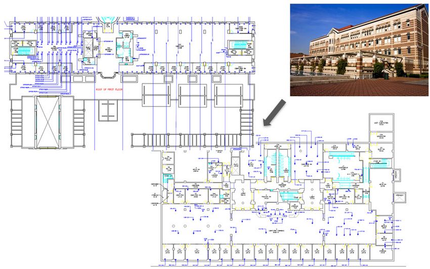
2                                                                            Jun-young Kwak et al.

1 Introduction

Reducing energy consumption is an important goal for sustainability. Thus, con-
serving energy in commercial buildings is important as it is responsible for signif-
icant energy consumption. In 2008, commercial buildings in the U.S. consumed 18.5
QBTU 1 , representing 46.2% of building energy consumption and 18.4% of U.S. en-
ergy consumption [21]. This energy consumption is significantly affected by a large
number of meetings or events in those buildings. The main drivers of such energy
consumption include HVAC (Heating, Ventilation, and Air Conditioning) systems,
lighting and electronic devices. Furthermore, a recent study shows that meeting fre-
quency in commercial buildings is significant and continues to grow [15]. In 2001,
U.S. Fortune 500 companies are estimated to have held 11 million formal meetings
daily and 3 billion meetings annually.
    Energy-oriented scheduling can assist in reducing such energy consumption [4,
36, 46]. Although conventional scheduling techniques compute the optimal schedule
for many meetings or events while satisfying their given requirements (i.e., comput-
ing a valid schedule) [12, 22, 31, 40], they have not typically considered energy con-
sumption explicitly. More recently, there have been some trials to conserve energy
by consolidating meetings in fewer buildings [26, 32]. In particular, Portland State
University consolidated night and weekend classes, which were previously scattered
across 21 buildings, into five energy efficient buildings. By doing this, they reported
that electricity consumption was reduced by 18.5% (78,000 kWh) in the autumn com-
pared to the previous three-year average. Similarly, Michigan State University con-
solidated classes and events into fewer buildings on campus, and energy reductions
in the seven buildings ranged from 2–20%, saving $16,904. However, these efforts
have been decided manually, and no underlying intelligent system was used.
    Motivated by this prior work, we describe TESLA (Transformative Energy-saving
Schedule-Leveraging Agent), an agent for optimizing energy use in commercial
buildings. TESLA is a goal-seeking (to save electric energy), continuously running
autonomous agent. TESLA’s key insight is that adding flexibility, which is a novel
concept for capturing user scheduling constraints, to meeting schedules can lead
to significant energy savings. Users in a commercial building continuously submit
meeting requests to TESLA while indicating flexibility in their meeting preferences.
TESLA schedules these meetings in the most energy efficient manner while ensur-
ing user comfort; but in cases where shifting meeting times can lead to significant
savings, TESLA interacts with users to request such a shift.
    Based on TESLA, this paper provides four key contributions. First, it provides
online scheduling algorithms, which are at the heart of TESLA, and presents the
sample average approximation (SAA) method [2, 29] to solve a two-stage stochastic
mixed integer linear program (SMILP). This SMILP considers the flexibility of peo-
ple’s preferences for energy-efficient scheduling of incrementally/dynamically arriv-
ing meetings and events. In this work, flexibility specifically refers to the number
of options made available by the user-specified scheduling constraints in terms of

 1 QBTU indicates Quadrillion BTU, which is used as the common unit to explain global energy use. 1

BTU = 0.00029 kWh.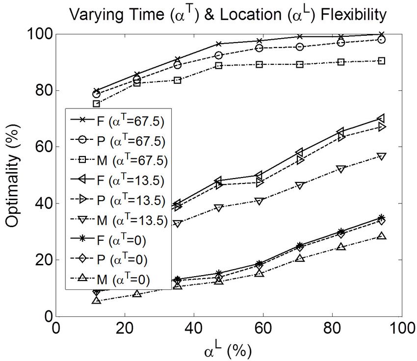
TESLA: An Extended Study of an Energy-saving Agent that Leverages Schedule Flexibility   3

starting time, locations and the deadline before committing to the finalized schedule
details. Second, TESLA also includes an algorithm to effectively identify key meet-
ings that could lead to significant energy savings by adjusting their flexibility. Third,
this paper provides an extensive analysis of the energy saving results achieved by
TESLA. Lastly, surveys of real users are provided indicating that TESLA’s savings
can be realized in practice by effectively leading people to change their schedule flex-
ibility. To validate our work, we used a public domain simulation testbed [21], fitted
it with details of our testbed building, and compared the simulation results against
real-world energy usage data. Our results show that, in a validated simulation us-
ing our testbed building, TESLA is projected to save about 94,000 kWh of energy
(roughly $18K) annually. Thus, TESLA can potentially offer energy saving benefits
to all commercial buildings where meetings affect energy usage.
     Although we have focused on evaluating TESLA in commercial buildings,
TESLA can be applied to general scheduling domains where schedule flexibility
plays a key role for conserving energy. For instance, while scheduling home appli-
ances in residential buildings [4, 28, 36, 44, 46], agents may consider people’s prefer-
ences and effectively adjust their appliance schedules (e.g., avoid running appliances
during peak hours) in order to save energy. Scheduling decentralized appliances in the
smart grid can be framed as a decentralized agent-based coordination problem, which
can be extended in distributing TESLA [13, 14, 42]. In addition, flexible scheduling
could be adopted for manufacturing systems as well [10, 38, 39] as there are many dif-
ferent sets of constraints/preferences while scheduling resources. In particular, spe-
cific temporal constraints on some activities such as local release dates (availability
of raw material) or due-dates (status review dates) are often flexible in practice, and
durations of activities are sometimes controllable, hence are a matter of preference as
well.
     The rest of the paper is organized as follows: In Section 2, we describe our testbed
buildings along with real data from those buildings. In Section 3, we describe the
TESLA system and the scheduling algorithms at the heart of it. Section 4 provides
evaluations for each of our algorithms using real-world meeting and energy data
which indicate that TESLA could potentially provide significant savings in overall
energy consumption. Section 5 discusses why TESLA works in detail by providing
an extensive analysis on energy savings. In Section 6, surveys of real meeting partic-
ipants are provided. Section 7 discusses a number of related approaches for handling
energy-aware scheduling. We conclude this paper in Section 8.
     This paper extends our AAMAS main track paper [19] and features a significant
amount of new material. First, Section 3.2.1 now formulates the online scheduling
problem as a stochastic mixed integer linear program (SMILP) in order to consider
various types of uncertainties as well as people’s flexibility. This formulation is more
expressive compared to our previous work, which presented a two-step process that
attempted to simulate an SMILP. In addition, we include a more general solution tech-
nique based on the sample average approximation (SAA) method to solve an SMILP.
Thus, we reran all the experiments using the SAA method with the same parameter
settings that were used in [19] and report new results in Section 4. Second, Sec-
tion 3.2.2 discusses the algorithm to identify key meetings not only independently
as in [19] but also simultaneously as a group. As we have shown in the evaluation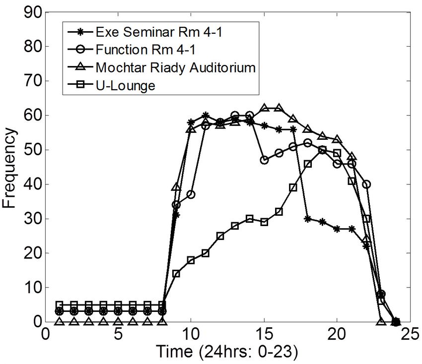
4                                                                  Jun-young Kwak et al.

Fig. 1 The actual research testbed (library) at USC

section, this change has significant potential to improve the overall energy savings.
Third, an extensive analysis on energy savings achieved by TESLA is provided in
Section 5, which will help readers understand why TESLA works in detail. This
analysis was absent in [19]. Fourth, analysis based on the collected meeting request
data from SMU (Figure 4) was included in Section 2.2. This analysis was not present
in our previous work. Fifth, Section 4 has been significantly enhanced with several
new major results. In addition to the new results on SAA that we discussed above,
major new additional results include: (i) the scalability and accuracy analysis of the
SAA method to solve the SMILP (Section 4.1.2); (ii) energy saving results based on
a different prediction heuristic for the predictive non-myopic method (SAA) (Section
4.1.3); (iii) energy saving improvements when simultaneously identifying multiple
key meetings (Section 4.1.4); (iv) further energy savings utilizing the cancellation
rate of meeting requests (Section 4.1.5); and (v) energy validation results to verify
the simulation environment (Section 2.1) and full energy saving results based on real
meeting data collected from SMU (Section 4.1.3). Sixth, Section 6 has been strength-
ened by providing (i) a set of questions used in questionnaire in our human subject
experiments (Tables 8 – 10) and (ii) further discussion regarding potential strate-
gic behaviors between agents and human users while focusing on a truthful and fair
mechanism at the end of Section 6. There are thus six significant areas of significant
improvement over our previous paper.
TESLA: An Extended Study of an Energy-saving Agent that Leverages Schedule Flexibility   5

Fig. 2 The current room reservation system at the testbed building

2 Research Testbed

2.1 Educational Building Testbed

Our system is to be deployed in an educational building. Figure 1 shows the testbed
building for TESLA’s deployment and the floor plans of 2nd and basement floors. It is
one of main libraries at the University of Southern California and has been designed
with a building management system. It hosts a large number of meetings (about 300
unique meetings per regular day) across 35 group study rooms. Each study room has
different physical properties including different types and numbers of devices and
facilities (e.g., video conferencing equipment, computer, projector, video recorder,
office electronic devices, etc.), room size, lighting specification, and maximum ca-
pacity (4 – 15 people). This building operates these study rooms 24 hours a day and
7 days a week except on national holidays. The temperature in group study rooms
is regulated by the facility managers according to two set ranges for occupied and
unoccupied periods of the day. HVAC systems always attempt to reach the pre-set
temperature regardless of the presence of people and their preferences in terms of
temperature. Lighting and appliance devices are manually controlled by users.
    In this building, meetings are requested by users by a centralized online room
reservation system (see Figure 2). In the current reservation system, no underlying
intelligent system is used; instead, users reactively make a request based on the avail-
ability of room and time when they access the system. While users make a request
using the system, they are asked about additional information including the number
of meeting attendees and special requirements. Reservations can be made up to 7
days in advance.
    Given the significant number of meetings per day and the centralized online meet-
ing reservation system, this library testbed provides a good environment to test vari-
ous energy-oriented scheduling techniques to mitigate energy consumption. TESLA’s
goal is to enable users to input flexibility in their scheduling request, to identify
key scheduling requests, and to use this information in algorithms that can provide
energy-efficient schedules to effectively conserve energy in commercial buildings.
To evaluate TESLA, we have built upon a simulation testbed [21] using real building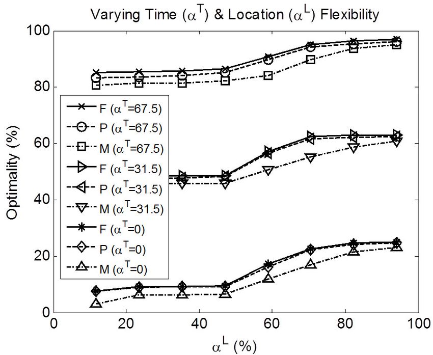
6 Jun-young Kwak et al.
Table 1 Energy consumption validation (kWh)
PP Period
PP Regular semester (Spring/Fall) Summer break Average
PP
Actual energy consumption 740.2 289.6 546.7
Simulated energy consumption 721.3 255.1 521.1
Average error (%) 2.6 11.9 4.7
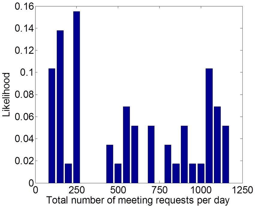
(a) Meeting frequency data (b) Distribution of total meeting requests per day
Fig. 3 Real data analysis (USC)
data and validated with real-world energy data (see Table 1). We specifically com-
pared the energy consumption calculated in the simulation testbed with actual energy
meter data from the testbed building (library) at the University of Southern Califor-
nia in 2012. As shown in Table 1, the average difference between actual energy meter
data and energy use from the simulation testbed was 4.7%, which strongly supports
our claim that the simulation testbed is realistic. This validated simulation environ-
ment is used to evaluate TESLA with real meeting data. In addition, we also test
TESLA on buildings at the Singapore Management University. SMU has a central-
ized web-based system that allows users to schedule meetings and events in over 500
conference/meeting rooms across eight buildings. More details regarding the data sets
from USC and SMU to test TESLA are provided in the next section.
2.2 Data Analysis
In collaboration with building system managers, we have been collecting data speci-
fying the past usage of group study rooms, which are collected for 8 months (January
through August in 2012) at USC. The data for each meeting request includes the time
of request, starting time, time duration, specified room, and group size. The data set
contains 32,065 unique meetings, and their average meeting time duration is 1.78
hours.
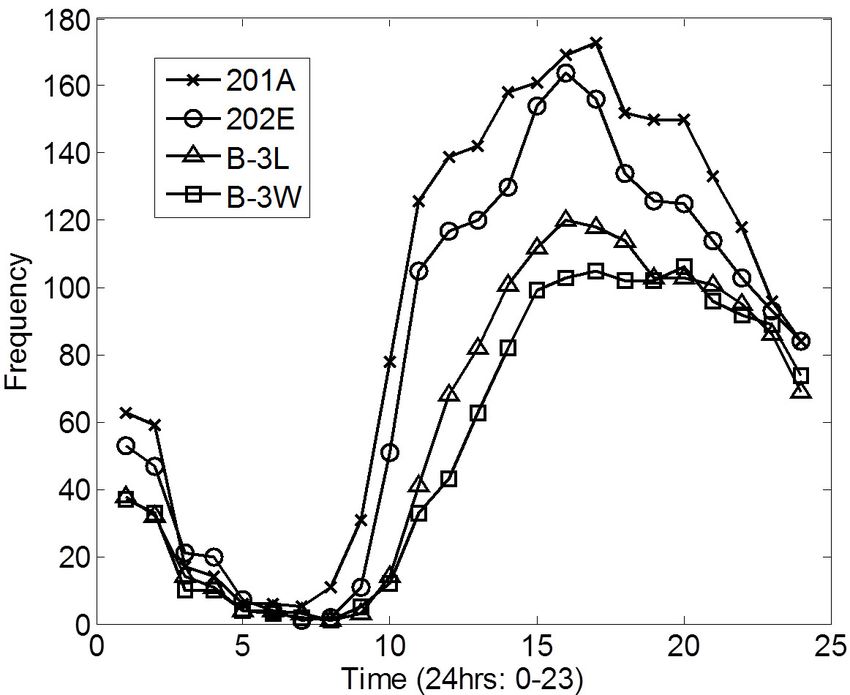
Figure 3(a) shows the actual meeting frequency (y-axis) over time (24 hours, x-
axis) of sampled 4 locations at USC (out of 35 rooms) based on the collected meeting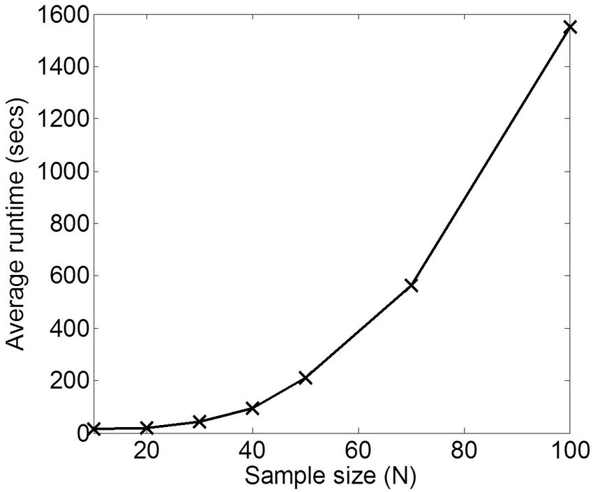
TESLA: An Extended Study of an Energy-saving Agent that Leverages Schedule Flexibility                7

Table 2 Meeting request arrival distribution
                                     Time period     Likelihood (%)
                                    1 day before         55.73
                                   1-2 days before       18.40
                                       2-3 days           8.72
                                       3-4 days           5.52
                                       4-5 days           3.68
                                       5-6 days           3.05
                                       6-7 days           3.35
                                      > 7 days            1.56

           (a) Meeting frequency data                (b) Distribution of total meeting requests per day

Fig. 4 Real data analysis (SMU)

request data. This figure shows the preferred slots of time and location (e.g., late af-
ternoon (2–5pm) for time & 2nd floor (201A, 202E) compared to the basement for
location). Then, the system will be able to predict future situations based on this fre-
quency data while scheduling requests as they arrive. Figure 3(b) shows the probabil-
ity distribution over total meeting requests per day. The x-axis of the figure indicates
the total number of meeting requests per day (ranging from 0 to about 350) and the
y-axis shows how likely the system will have the given number of total meeting re-
quests (x-axis) on one day. One can see that the probability of having 50 or fewer
meetings is 42.92% and the probability of having 250 or more meetings is 30.04%.
These are used to estimate the model of future meetings in our algorithm that will be
presented in Section 3.2.
    Table 2 shows how early meeting requests were made. In the table, column 2
indicates the percentage of meetings that were requested within the given time period
(column 1). For instance, 55.73% of all meeting requests were made within 1 day
before the actual meeting day. This analysis would be helpful in understanding how
our algorithm could achieve significant energy savings in this domain.
    While evaluating TESLA, we also consider another data set from SMU. The data
set contains over 80,000 meetings that have been collected for three months (August
through October) in 2011 at SMU, which gives us a sense regarding how TESLA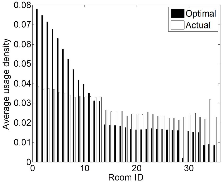
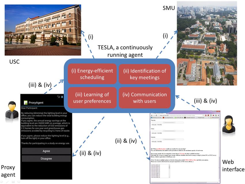
8                                                                                     Jun-young Kwak et al.

Fig. 5 TESLA architecture: TESLA is a continuously running agent that supports four key features: (i)
energy-efficient scheduling; (ii) identification of key meetings; (iii) learning of user preferences; and (iv)
communication with users.

will handle energy-oriented scheduling problems in large buildings. Similar to Fig-
ure 3, Figure 4(a) shows the actual meeting frequency (y-axis) over time (24 hours,
x-axis) of sampled 4 locations at SMU (out of over 500 rooms) based on the collected
meeting request data. This figure shows the preferred slots of time and location. Fig-
ure 4(b) shows the probability distribution over total meeting requests per day. The
x-axis of the figure indicates the total number of meeting requests per day (ranging
from 0 to about 1200) and the y-axis shows how likely the system will have the given
number of total meeting requests (x-axis) on one day.

3 TESLA

In this section, we describe the overall architecture of TESLA and how to optimally
schedule meetings in real-world situations to conserve energy in commercial build-
ings.

3.1 TESLA Architecture

TESLA is a goal-seeking (to save energy), continuously running autonomous agent.
TESLA performs on-line energy-efficient scheduling while considering dynamically
arriving inputs from users; these dynamic inputs make the scheduling complex and
TESLA needs to learn a predictive model for users’ inputs and preferences (see Fig-
ure 5). More specifically, TESLA:
TESLA: An Extended Study of an Energy-saving Agent that Leverages Schedule Flexibility                9

 – takes inputs (i.e., preferred time, location, the number of meeting attendees, etc.)
   from different users and their proxy agents at different times (Sections 2 & 3.1)
 – autonomously performs on-line energy-efficient scheduling as requests arrive
   while balancing user comfort (Section 3.2.1)
 – autonomously, on own initiative, interacts with different users based on identified
   problematic key meetings in order to avoid bother cost to users while persuading
   them to change meeting flexibility (Section 3.2.2)
 – bases its non-myopic optimization on learned patterns of meetings (Sections 3.2.1
   & 4)
    As shown in Figure 5, meeting requests are the information we get from the inter-
face of TESLA via the web interface (or via a proxy agent [34] on an individual user’s
hand-held device, in case the users have proxy agents, who have the corresponding
users’ preferences and behavior models with a certain level of adjustable autonomy).
TESLA focuses on minimizing unnecessary interactions by detecting a small number
of key meetings while negotiating with people to adjust their flexibility. TESLA may
interact with users’ proxy agents instead of the users themselves.

3.2 TESLA Algorithms

The objective of this work is to come up with energy efficient schedules in commer-
cial buildings with a large number of meetings while considering (i) flexibility in
meeting requests over time, location and deadline; and (ii) user preferences with re-
spect to energy and satisfaction. To account for these two constraints, we provide two
types of algorithms, which are at the heart of TESLA. First, we provide algorithms
that compute a schedule for known and predicted meeting requests which have flex-
ibility in time, location and deadline. Second, based on the schedule obtained, we
provide algorithms that detect meeting requests which if modified (to increase flexi-
bility) can result in significant energy savings.

3.2.1 Scheduling algorithms

Before describing our scheduling algorithms, we formally describe the scheduling
problem. Let T represent the entire set of time slots available and L represent the
set of available locations each day. A schedule request ri is represented as the tuple:
ri =< ai , Ti , Li , δi , di , ni >, where: ai is the arrival time of the request, Ti ⊂ T is
the set of preferred time slots for the start of the event and Li ⊂ L is a set of preferred
locations. di is the deadline by which the time and location for the meeting should
be notified to the user, δi is the duration for the event and finally, ni is the number of
attendees.
    The flexibility of the meeting request ri is a tuple denoted by αi : < αiT , αiL ,
  d
αi >.2
  2 Flexibility is already present in the meeting request as its constraints, and α is a measure of such

constraints.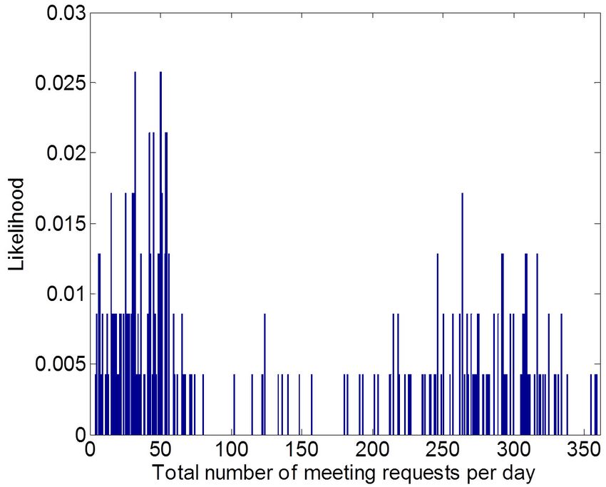
10                                                                      Jun-young Kwak et al.

Fig. 6 Disjoint sets of R

                                                 |Ti |−1
 – αiT : time flexibility of meeting i. αiT = |T   |−δi × 100 (|T | > δi ; i.e., |T | is 24
   hours per day).
 – αiL : location flexibility of meeting i. αiL = |L  i |−1
                                                    |L|−1 × 100 (|L| > 1).
                                                    di −ai
 – αid : deadline flexibility of meeting i. αid =   d∗       × 100, where d∗i is the latest
                                                     i −ai
     notification time (e.g., midnight on the meeting day) (d∗i > ai ). 0 ≤ αid ≤ 100

    For instance, given only one time slot (|Ti | = 1), αiT = 0 and all available time
slots (|Ti | = |T | − δi + 1), αiT = 100. Assuming that people give Ti = 4–7pm on
Monday and their meeting time duration is 2 hours, then αiT = (4-1)/(24-2) × 100
= 13.64%. Likewise, given only one location slot (|Li | = 1), αiL = 0 and given all
available locations (|Li | = |L|), αiT = 100.
    We now define specific disjoint sets of meeting requests, R, that will enable us to
characterize different types of scheduling algorithms, where t is the time to schedule
a given set of requests R.

 – RS (t) = {i : di = t and ai ≤ t}: a set of requests that have to be scheduled at
   time t
 – RA (t) = {i : di < t and ai < t}: a set of requests that were assigned before time
   t
 – RK (t) = {i : di > t and ai ≤ t}: a set of known future requests, which arrived
   before time t, but will be scheduled in the future
 – RU (t) = {i : di > t and ai > t}: a set of unknown future requests

    As a simple example (shown in Figure 6), let us consider that we have 4 meet-
ing requests (r1 , r2 , r3 , and r4 ), which are supposed to be scheduled on the same
day. The current time is t. According to the definition, RS (t) = {r2 }, RA (t) =
{r1 }, RK (t) = {r3 }, and RU (t) = {r4 }.
    Given a set of requests, R, we provide a two-stage stochastic mixed integer linear
program (SMILP) to compute a schedule that minimizes the overall energy consump-
tion. Stochastic programming has provided a framework for modeling optimization
problems that involve uncertainty [6, 9, 16, 35]. Whereas deterministic optimization
problems are formulated with known parameters, real world problems almost in-
variably include some unknown parameters. In particular, our scheduling problem
aims to optimally schedule incrementally/dynamically arriving requests, and thus we
should consider uncertainty in terms of future requests, which makes deterministic
TESLA: An Extended Study of an Energy-saving Agent that Leverages Schedule Flexibility 11
optimization techniques inapplicable. To address this challenge, we specifically for-
mulate our scheduling problem as a two-stage stochastic program. Here the decision
variables are partitioned into two sets. The first stage variables are decided before the
actual realization of the uncertain parameters are known. Afterward, once the random
events have exhibited themselves, further decisions can be made by selecting the val-
ues of the second stage. The second stage decision variables can be made to minimize
penalties that may occur as a result of the first stage decision. This SMILP will be run
every time a new meeting request arrives (or after a batch of meeting requests arrive
in close succession).
The notation that will be employed in the SMILP is as follows:
– xil,t is the first stage binary variable that is set to 1 if meeting request ri is sched-
uled in location l starting at time t.
i
– El,t is a constant that is computed for a meeting request ri if it is scheduled in
location l at time t using the HVAC energy consumption equations.
– C is a constant that indicates the reduction in energy consumption because of
scheduling a meeting in the previous time slot. Although we assumed that C is
a constant for simplicity in this work, it depends on different factors of previous
meetings in practice.
– eil,t is a continuous variable that corresponds to the energy consumed because of
scheduling meeting i in location l at time t. The value of this variable is affected
based on whether there is a meeting scheduled in the previous time slot (t−1), i.e.,
the reduction that would occur at location l at time P t if a meeting was scheduled
0
at location l at time t − 1. 3 eil,t = xil,t · El,t
i
− i0 ∈R\{i} xil,t−1 · C.
i
– Sl,t is a value that indicates the satisfaction level obtained with users in meeting
request ri for scheduling the meeting in location l at time t. B is a threshold on
the satisfaction level required by users.
– M is an arbitrarily large positive constant.
– Q(x, ξ) is the value function of future energy consumption, where ξ represents
uncertainty over the second stage problem (i.e., future meeting situations in our
problem). ξ determines a vector of parameters, (w, q).
j
– wl,t is the second stage binary variable that is set to 1 if meeting request rj in a
future meeting request set is scheduled in location l starting at time t.
j
– ql,t is a continuous second stage variable that corresponds to the future energy
consumed because of scheduling meeting j in location l at time t.
We first provide the SMILP and a detailed explanation of the constraints.
3 ei gets affected by a meeting in the previous time slot in the same location. This is because adjacent
l,t
meetings affect the indoor temperature, which makes HVACs operate differently to maintain the desired
temperature level.12 Jun-young Kwak et al.
min e + E[Q(x, ξ)] (1)
{Choose the optimal first stage variables that minimizes the sum of first stage costs
and the expected value of the second stage}
s.t.
X XX
e≥ eil,t , (2)
i∈R\RU t∈T l∈L
{Computing the first stage cost e}
X 0
eil,t = xil,t · El,t
i
− xil,t−1 · C, ∀i ∈ R \ RU , l ∈ L, t ∈ T (3)
i0 ∈R\RU \{i}
{Computing energy consumption while considering the back-to-back meeting effect}
eil,t ≥ 0, ∀i ∈ R \ RU , l ∈ L, t ∈ T (4)
XX
xil,t · Sl,t
i
≥ B, ∀i ∈ R \ RU (5)
t∈T l∈L
{Checking if the computed schedule maintains the given comfort level B}
X
xil,t ≤ 1, ∀l ∈ L, t ∈ T (6)
i∈R\RU
t+δi −1
X X 0
xil,t0 ≤ M (1 − xil,t ), ∀l ∈ L, i ∈ R \ RU , t ∈ T (7)
i0 ∈R\RU \{i} t0 =t
{Checking the allocation restrictions that for each assignment slot, only one meeting
can be scheduled considering the given time duration of meeting}
xil,t ∈ {0, 1}, ∀i ∈ R \ RU , l ∈ L, t ∈ T (8)
{The first stage binary variable}
X XX j
Q(x, ξ) ≥ ql,t , (9)
j∈RU l∈L t∈T
{Computing the second stage cost Q}
X X X 0
j j j j
ql,t = wl,t · El,t − xil,t−1 · C − xil,t+1 · C − wl,t−1 · C,
i∈R\RU i∈R\RU j 0 ∈RU \{j}
(10)
{Computing energy consumption while considering the back-to-back meeting effect
caused by the first and second stage variables}
j
ql,t ≥ 0, ∀j ∈ RU , l ∈ L, t ∈ T (11)
X j
wl,t ≤ 1, ∀l ∈ L, t ∈ T (12)
j∈RU
X t+δ
X i −1
j i
wl,t0 ≤ M (1 − xl,t ), ∀l ∈ L, i ∈ R \ RU , t ∈ T (13)
j∈RU t0 =t
{Checking the allocation restrictions against the first stage assignment slots}
t+δj −1
X X 0
j j
wl,t0 ≤ M (1 − wl,t ), ∀l ∈ L, j ∈ RU , t ∈ T (14)
j 0 ∈RU \{j} t0 =t
{Checking the allocation restrictions against the second stage assignment slots}
j
wl,t ∈ {0, 1}, ∀j ∈ RU , l ∈ L, t ∈ T (15)
{The second stage binary variable}TESLA: An Extended Study of an Energy-saving Agent that Leverages Schedule Flexibility 13
The objective of the SMILP above is to choose the optimal first stage variables
(i.e., the optimal assignment of meeting requests to locations and time slots that is
∗
characterized by the solution, xil,t ). The optimal first stage variable, x∗ , is selected
in a way that the sum of first stage costs e (i.e., the energy consumption when the
current meeting request is scheduled) and the expected value of the second stage or
recourse costs E[Q(x, ξ)] (i.e., the expected energy consumption that will be realized
by future meeting requests) is minimized. In this formulation, at the first stage we
have to make a decision before the realization of the uncertain data ξ, which is viewed
as a random vector that determines future meeting requests, is known. At the second
stage, after a realization of ξ becomes available, we optimize our behavior by solving
an appropriate optimization problem.
Constraints (2) – (8) are a set of enforcement for deciding first stage variables,
and constraints (9) – (15) enforce conditions for second stage variables. More specif-
ically, constraint (3) is for computing energy consumption considering the back-to-
back meeting effect. In particular, we subtract from the energy consumed by this
meeting indexed by i at time t, the impact due to meetings (indexed by i0 ), that were
scheduled at the prior time slot t − 1. Constraint (5) is for checking if the computed
schedule maintains the given comfort level B. Constraints (6) and (7) are the allo-
cation restrictions that for each assignment slot, only one meeting can be scheduled
considering the given time duration of meeting. In particular, M in constraint (7) is
an arbitrarily large positive constant to enforce only one meeting is scheduled at a
location during the duration of the meeting. If meeting i is assigned to location l and
time t (xil,t = 1), then any other meeting requests cannot be assigned to the same
slot. If xil,t = 0, the constraint does not block any other meeting requests from being
assigned to that slot as the right-hand side of the equation is not bounded due to an
arbitrarily large constant of M . Constraint (9) is to compute the optimal value of the
second stage problem while satisfying constraints (10) – (15) which are similar to
constraints (3) – (8). Specifically, constraint (10) is for computing the energy reduc-
tion that would occur if there are any consecutive meetings among the requests in
RU (i.e., check with w) and if any future meetings have this back-to-back effect with
either already assigned meetings or ones that have to be scheduled in R \ RU (i.e.,
check with x).
We now describe the sample average approximation (SAA) method [2, 29] to
solve the given SMILP. The main idea of the SAA approach to solve stochastic pro-
grams is as follows. A sample ξ 1 , . . . , ξ N realizations of the random vector ξ is gen-
erated, and consequently the expected value function E[Q(x, ξ)] in the stochastic
PN
program (1) is approximated by the weighted average function n=1 pU n
n Q(x, ξ ),
where pU n is the likelihood that ξ n
is realized. Recall that ξ is the random vector that
determines future meeting requests in our formulation (i.e., each realization ξ n has a
different number of future meeting requests and corresponding request tuples). More
specifically, we have a probability distribution pT over the possible range of total
meeting requests per day (shown in Figures 3(b) & 4(b)). Then, the likelihood that k
more meetings will arrive on the same day assuming we currently have s meetings so
far is equivalent to the likelihood that ξ n is realized with k unknown future requests:
pU T U
n (k) = p (s + k). For those k future meeting requests in Rn , we generate random14 Jun-young Kwak et al.
request tuples (specifically, Ti & Li ) based on the actual distribution over the assign-
ment spots as shown in Figures 3(a) & 4(a). Then, for a sample n (1 ≤ n ≤ N ), the
original SMILP is reformulated as follows:
N
X
min e + pU n
n Q(x, ξ ) (16)
n=1
{Using SAA, the expected value of the second stage cost is approximated by
the weighted average function. Then, we still choose the optimal first stage
variable that minimizes the sum of the first and second stage costs}
s.t.
Constraints (2) – (8),
X XX
Q(x, ξ n ) ≥ n
qj,l,t , (17)
U l∈L t∈T
j∈Rn
X X X
n n
qj,l,t = wj,l,t · Ej,l,t − xi,l,t−1 · C − xi,l,t+1 · C − wjn0 ,l,t−1 · C,
i∈R\RU i∈R\RU j 0 ∈Rn
U \{j}
(18)
n
qj,l,t ≥ 0, ∀j ∈ RnU , l ∈ L, t ∈ T (19)
X
n
wj,l,t ≤ 1, ∀l ∈ L, t ∈ T (20)
U
j∈Rn
X t+δ
X i −1
n
wj,l,t0 ≤ M (1 − xi,l,t ), ∀l ∈ L, i ∈ R \ RU , t ∈ T (21)
U
j∈Rn t0 =t
t+δj −1
X X
wjn0 ,l,t0 ≤ M (1 − wj,l,t
n
), ∀l ∈ L, j ∈ RnU , t ∈ T (22)
j 0 ∈Rn
U \{j} t0 =t
n
wj,l,t ∈ {0, 1}, ∀j ∈ RnU , l ∈ L, t ∈ T (23)
N
X
pU
n =1 (24)
n=1
{pU
n is the likelihood that ξ n is realized, where ξ is a random variable that
determines future meeting requests U }
The obtained sample average approximation (16) of the stochastic program is
then solved using a standard branch and bound algorithm such as those implemented
in commercial integer programming solvers such as CPLEX.
As benchmark algorithms for comparison purposes, we provide two optimiza-
tion heuristics: myopic and full-knowledge. We have the myopic optimization al-
gorithm, which obtains a schedule by considering the following request set: R =
(RA (t) ∪ RS (t) ∪ RK (t)). A schedule and energy consumption are obtained withoutTESLA: An Extended Study of an Energy-saving Agent that Leverages Schedule Flexibility 15
accounting for future unknown meetings. Thus, the myopic heuristic only considers
the first stage decision variables in our SMILP. In the full-knowledge method, we
compute the final schedule while assuming that the entire set of meeting requests R
is given, which is ideal. Thus, for the full-knowledge method, we have one actual
realization with probability 1.0 for computing the second stage costs in the SMILP.
The performance comparison results will be provided in Section 4.
3.2.2 Identifying key meetings
TESLA computes the optimal schedule considering the given flexibility (or schedul-
ing constraints) of meetings. It can obtain more energy-efficient schedules by increas-
ing flexibility (i.e., relaxing those constraints). We now provide an algorithm that
finds meeting requests, which if made more flexible will reduce energy consumption
significantly.
Algorithm 1 I DENTIFY K EY M EETINGS (R)
1: U←∅
2: {Initialize a set of key meetings}
3:
4: for all I ⊂ 2R do
5: {R is a set of requests.}
6: if I S S AVING C ANDIDATE (I) then
7: U←U∪I
8:
9: return U
Algorithm 1 describes the overall flow of the algorithm. We first initialize a set
that will contain key meetings identified by our algorithm (line 1). For each subset
of the power set of meeting requests R, we then examine whether or not the current
meeting set I is a key meeting set by relying on Algorithm 2 (line 6).
Algorithm 2 recursively determines if the given meeting set I is a candidate set
that gives significant potential energy savings. The meeting set I is detected as a key
meeting set only if the expected energy savings of meeting requests in I are mono-
tonically increasing and show higher energy improvements than the given threshold
value (τ ; a certain level of additional energy savings that we desire to achieve with the
selected key meetings) by relaxing their flexibility. To handle this, we first compute
the expected energy savings of the meeting set I when its flexibility level is changed
from the initial level αI to the desired level αI0 assuming the other meetings’ flex-
ibility levels are fixed (line 1). The expected energy saving value of meeting set I,
VI = (EαI − Eα0I )/EαI (0 ≤ VI ≤ 1), where EαI is the current total energy con-
sumption with the given level of flexibility αI , and Eα0I is the reduced total energy
consumption if the meeting set I’s flexibility is changed to one of k possible op-
0
tions, αI,k , while others keep their given flexibility levels. In this work, we consider
a heuristic for setting the threshold value to investigate whether or not the current
meeting set I is an energy saving candidate set: a fixed single threshold value τ (line
5; e.g., 0.4 as a universal threshold).16 Jun-young Kwak et al.
Algorithm 2 I S S AVING C ANDIDATE (I )
1: VI ← C AL E XP E NERGY S AVINGS (αI , {α0I,1 , . . . , α0I,k })
2: {αI is an initially given flexibility of meetings in I, and α0I,k is one of the desired flexibility options
for meetings in I. C AL E XP E NERGY S AVINGS computes energy gains, VI , by relaxing flexibility of
meeting requests in I.}
3:
4: if |I| = 1 then
5: if VI > τ then
6: {If the computed energy gains VI is higher than a given threshold value τ , it is considered as a
key meeting.}
7: return TRUE
8: else
9: return FALSE
10: else if |I| > 1 then
11: {Recursively call I S S AVING C ANDIDATE with possible subsets}
12: for all i ∈ I do
13: I’ ← I\{i}
14: VI 0 ← C AL E XP E NERGY S AVINGS (αI 0 , {α0I 0 ,1 , . . . , α0I 0 ,k })
15: if VI − VI 0 > 0 then
16: {Only if the energy savings are monotonically increasing by adding a meeting request i (or
monotonically decreasing by excluding a meeting request i), proceed}
17: return I S S AVING C ANDIDATE (I 0 )
4 Empirical Validation
We evaluate the performance of TESLA and experimentally show that it can conserve
energy by providing more energy-efficient schedules in commercial buildings. At
the end of this section, we provide actual survey results that we have conducted on
schedule flexibilities of real users. The experiments were run on Intel Core2 Duo
2.53GHz CPU with 8GB main memory. We solved our MILP formulations using
CPLEX version 12.1. All techniques were evaluated for 100 independent trials and
we report the average values. Energy consumption was computed using the simulator
described earlier in Section 2.1.
4.1 Simulation Results
In this section, we provide the simulation results (i) to verify if flexibility really helps
TESLA compute energy-efficient schedules; (ii) to extensively evaluate the overall
performance of the SAA method while varying the sample size and flexibility; and
(iii) to measure energy saving benefits by identifying key meetings and by consider-
ing the cancellation rate.
4.1.1 Does flexibility help?
As an important first step in deploying TESLA, we first verified if the agent could
save more energy with more flexibility while scheduling given meeting and event
requests. To that end, we compared the energy consumption of three different ap-
proaches using the real-world meeting data mentioned in Section 2.2: (i) the currentTESLA: An Extended Study of an Energy-saving Agent that Leverages Schedule Flexibility 17
Fig. 7 Energy savings: Actual - the amount of energy consumed in simulation based on the past schedules
obtained from the current manual reservation system; Random - energy consumption while randomly
perturbing the starting time and location of meeting requests from the same past schedules while keeping
meeting time duration; Optimal - Energy consumption measured in simulation based on optimal schedules
computed from an SMILP with the fully known meeting request set and full flexibility
benchmark approach in use at the testbed building; (ii) a random method that ran-
domly assigns time and location for meetings; and (iii) the optimal method using the
full-knowledge optimization technique described in Section 3.2.
Figure 7 shows the average daily energy consumption in kW h computed based
on schedules from the three algorithms above. In the figure, the consumption is the
amount of energy consumed based on the past schedules obtained from the cur-
rent manual reservation system, which shows a very similar performance to the ran-
dom approach. The optimal method assuming the full amount of flexibility (i.e., 24
hours for αT , 35 rooms for αL and delay the deadline before which the final sched-
ule should be informed for αd ) achieved statistically significant energy savings of
50.05% compared to the current energy consumption at the testbed site. These sav-
ings are practically significant, and also statistically significant (paired-sample t-test;
p < 0.01). These savings are equivalent to annual savings of about $18,600 consid-
ering an energy rate of $0.193/kWh [41] and CO2 emissions from the energy use of
5.5 homes for one year. Thus, flexibility can help save energy.
4.1.2 Online scheduling method with flexibility: Determining the sample size in the
TESLA SMILP
In this section, we first investigated the runtime and solution qualities for solving the
SMILP while varying the number of samples (see Figure 8). Figure 8(a) shows the
results of the runtime analysis in seconds (y-axis) for sample sizes N = 10 to 100
(x-axis). As shown in the figure, the runtime increases in an exponential fashion as
the sample size N increases. However, Figure 8(b) shows that its solution quality
also increases (y-axis) (i.e., the estimated optimality gap decreases) as the number of
samples N increases. For evaluating the generated solution for each of sample size18 Jun-young Kwak et al.
(a) Scalability: runtime (b) Accuracy: average error
Fig. 8 Scalability and accuracy while varying the number of samples (N)
Fig. 9 Energy savings while varying flexibility (USC)
N , we generated M independent samples (i.e., replications) of the uncertain param-
eters, and evaluated the obtained solution in each m ∈ M replication. In this work,
we specifically used 1,000 independent replications for measuring the estimated op-
timality. Comparing the full-knowledge schedules based on actual realization of each
of the 1000 samples with the schedule from the SMILP gives us the percentage error.
Based on this result, throughout the paper, we set N = 50 to solve the SAA prob-
lem. This sample size has a reasonable runtime without a significant compromise in
solution quality.
4.1.3 Performance of online scheduling method with flexibility
We next compared solution qualities of the three scheduling algorithms in TESLA
presented in Section 3.2.1. Figure 9 shows that how much each algorithm saves whenTESLA: An Extended Study of an Energy-saving Agent that Leverages Schedule Flexibility 19
Table 3 Performance comparison between SAA and myopic
H
HH Max Min Average
H
Optimality difference 57.89% 0.50% 12.73%
compared to the optimal value (i.e., full-knowledge optimization assuming the full
flexibility) while varying the time and location flexibility level (assuming 0% dead-
line flexibility). The flexibility in our model represents a 3-dimensional space (time,
location and deadline), which we have thoroughly explored. We show results explor-
ing deadline flexibility later.
The optimality percentage on the y-axis of Figure 9 is computed as follows: (Ea −
Ec )/(Ea − Eo ). Here Ea is the actual energy consumption without any flexibility,
Eo is the optimal energy consumption, and Ec is the computed energy consumption
using three different scheduling algorithms that we compare using the real meeting
data.
Figure 9 shows the average optimality in percentage of each algorithm (M: my-
opic, P: predictive non-myopic (SAA) and F: full-knowledge) while varying the loca-
tion flexibility (αL ; x-axis) and time flexibility (αT ; each graph assumed the different
amount of αT as indicated in the legend). In the figure, for each pair of flexibility val-
ues (αT , αL ), we report the average optimality in percentage (i.e., 100% indicates the
optimal value, and 0% means that there was no improvement from the actual energy
consumption). For instance, when flexibility (αT , αL ) = (31.5%, 58.8%), the myopic
method achieved an optimality of 50.8%. In the figure, higher values indicate better
performance.
As shown in Figure 9, as users provide more flexibility, TESLA can compute
schedules with less energy consumption. The gain in optimality from myopic to pre-
dictive non-myopic (SAA) is because the latter can leverage user flexibility to put a
meeting in a suboptimal spot at the meeting request time to account for future meet-
ings, yielding better results at the actual day of meetings. For example, a flexible
meeting request can be moved away from a known popular time-location spot. We
conclude that (i) the predictive non-myopic (SAA) method is superior to the myopic
method. Table 3 shows the average performance comparison results between the pre-
dictive non-myopic (SAA) method and the myopic technique. As shown in the table,
the maximum and average optimality differences between the two methods (i.e., opti-
mality of the SAA - optimality of the myopic) are 57.89% and 12.73%, respectively,
which are significant. In addition, for 12.50% of cases, the predictive non-myopic
(SAA) optimization showed over 20% higher optimality than the myopic method;
(ii) the predictive non-myopic (SAA) method performs almost as well as the full-20 Jun-young Kwak et al.
Table 4 % of optimal energy savings: varying αT , αL , and pf (USC)
Location flexibility (αL )
Alg. pf 23.5 47.1 70.6 94.1
1.0 6.6 6.7 17.8 23.3
0.8 5.6 6.0 14.5 21.2
M
0.5 4.9 4.9 13.8 18.2
0.2 3.3 3.8 8.4 12.0
1.0 9.7 9.8 22.7 24.8
0.8 8.6 9.3 20.9 23.2
0 P
0.5 6.4 6.9 15.6 18.6
0.2 4.2 4.9 9.8 12.9
1.0 9.9 10.1 23.6 25.8
0.8 8.3 8.6 20.7 24.0
T. flex. (αT ) F
0.5 6.7 6.9 16.9 19.1
0.2 4.9 5.1 11.3 13.6
M 1.0 46.3 46.5 55.8 61.4
P 1.0 48.1 48.5 62.1 62.7
1.0 49.0 49.2 63.0 63.1
31.5
0.8 41.9 43.3 55.5 57.6
F
0.5 29.9 30.7 43.9 44.5
0.2 16.1 16.7 26.9 27.2
M 1.0 81.8 82.5 89.6 96.0
P 1.0 84.4 86.3 95.4 96.8
1.0 86.3 86.8 96.0 97.5
67.5
0.8 73.3 73.5 87.9 91.3
F
0.5 53.7 54.4 65.0 67.8
0.2 29.4 30.6 38.2 41.4
(M: myopic, P: predictive non-myopic (SAA), F: full-knowledge)
knowledge optimization (about 98%) 4 ; and (iii) full flexibility is not required to start
accruing benefits of flexibility.
In the real-world, it is hard to imagine that all people will simply comply and
change their flexibility to achieve such optimality. Thus, we provide one additional
result shown in Table 4 which varies the percentage of meetings that will have flexi-
bility (pf ). We show αT along the rows and αL along the columns. In particular, the
value of row 10 and column 5 (highlighted in the table) shows the optimality achieved
by the predictive method assuming that 20% of meetings (randomly selected) have
(αT , αL ) = (0%, 23.5%) flexibility and the remaining 80% have no flexibility. Our
main conclusions are: (i) if we increase pf , we are able to achieve a higher optimal-
ity; and (ii) flexibility in a small number of meetings can lead to significant energy
reduction. This motivates considering more intelligent identification of key meetings
to change their flexibility (described in the next section).
We also compared the performance of the three algorithms while varying the
deadline flexibility, αd . In Table 5, columns indicate different amounts of deadline
4 The average performance of the predictive non-myopic (SAA) optimization depends on the prediction
method of future requests. We, thus, additionally tested a more sophisticated prediction method considering
the time factor that is one of key features determining the overall trend of requests (i.e., when the meeting
requests arrive at the system to be scheduled; e.g., regular semester vs. summer/ winter break). With this
additional consideration, the predictive non-myopic (SAA) method improved the overall performance of
the predictive method by 1.1%.TESLA: An Extended Study of an Energy-saving Agent that Leverages Schedule Flexibility 21
Table 5 Percentage of optimal energy savings: varying αd (USC)
PP α d
P 0.0 22.2 44.4 66.7 88.9
Alg. PP
P
M 82.5 83.4 84.0 84.2 84.2
P 86.3 86.4 86.7 86.7 86.8
F 86.8 86.8 86.8 86.8 86.8
(M: myopic, P: predictive non-myopic (SAA), F: full-knowledge)
Fig. 10 Energy savings while varying flexibility (SMU)
Table 6 Percentage of optimal energy savings: varying αd (SMU)
d
P α
PP
0.0 22.2 44.4 66.7 88.9
Alg. PPP
M 85.30 87.22 89.02 89.41 90.06
P 93.01 93.05 94.56 94.87 95.14
F 95.21 95.21 95.21 95.21 95.21
(M: myopic, P: predictive non-myopic (SAA), F: full-knowledge)
flexibility and values are the optimality of each algorithm assuming a fixed time and
location flexibility (αT , αL ) = (67.5%, 47.1%). As we increase the deadline flexi-
bility, both myopic and predictive non-myopic (SAA) methods converge to the full-
knowledge optimization result. This is because as the deadline flexibility increases,
we can delay scheduling until we have more information. In this particular case of
αT and αL , we do not necessarily see significant benefits by providing more dead-
line flexibility since the myopic and predictive non-myopic (SAA) methods already
achieved fairly high optimality compared to the full-knowledge method. While the
optimality percentage changes are small, given the vast amount of energy consumed
by large-scale facilities, these reductions can lead to significant energy savings. We
are investigating conditions where our algorithms get more benefits by deadline flex-
ibility.22 Jun-young Kwak et al.
Table 7 Energy improvement of identified key meetings (%)
H α
H
(0,23.5) (0,47.1) (0,70.6) (31.5,23.5) (31.5,47.1)
α0 HH
(0,23.5) - - - - -
(0,47.1) 16.08 - - - -
(0,70.6) 30.08 29.17 - - -
(31.5,23.5) 32.05 - - - -
(31.5,47.1) 46.18 36.27 - 29.17 -
(31.5,70.6) 46.52 38.33 34.36 31.07 26.08
The same types of analysis are performed with another data set from SMU and
results are presented in Figure 10. The figure shows the average optimality in per-
centage of each algorithm (M: myopic, P: predictive non-myopic (SAA) and F: full-
knowledge) on the y-axis while varying the time flexibility (αT ; each graph assumed
the different amount of αT as indicated in the legend) and location flexibility (αL ;
x-axis). We assume the deadline flexibility (αd ) of 0%. Similar to earlier results, the
predictive method achieved about 97% optimality compared to the full-knowledge
optimization and showed higher value than the myopic approach. We also compared
the performance of the three algorithms while varying the deadline flexibility. In Ta-
ble 6, values are the optimality of each algorithm assuming a fixed time and location
flexibility, (31.5%, 47.1%). Here we see more pronounced energy savings at SMU as
αd increases compared to the USC results.
4.1.4 Performance of identifying key meetings
We evaluated the performance of the algorithm to identify key meetings for energy
reduction. In our tests, we selected 10 meetings individually using the algorithm pre-
sented in Section 3.2.2 and calculated the average energy savings if those selected
meetings changed their flexibility.
Table 7 shows the average energy savings as described for various flexibility tran-
sitions. Columns indicate the initial level of flexibility (α = (αT , αL )) and rows show
the requested level of flexibility (α0 = (α0T , α0L )). For instance, the value in row 4
and column 3 (highlighted in the table) indicates a 29.17% average energy savings
improvement if flexibility of 10 key meetings are changed from (0%, 47.1%) to (0%,
70.6%). An important interpretation of that results is that changing the flexibility of
key meetings, when those ones are from an appropriately chosen set, contributed to
significant energy savings. We also tested how much we can save energy if we choose
key meetings simultaneously rather than independently. Assuming the current flexi-
bility is (0%, 23.5%) (column 2 in Table 7), if we choose 10 key meetings at the same
time using the same algorithm presented in Section 3.2.2, the average energy savings
were improved by 10.3% (i.e., 44.48% of energy saving improvements on average).
In the future, we will investigate another heuristic to set a feasible threshold value
based on a learned profile of user likelihood of changing meeting flexibility.TESLA: An Extended Study of an Energy-saving Agent that Leverages Schedule Flexibility 23
Fig. 11 Average energy improvement while considering the cancellation rate of meeting requests
4.1.5 Considering the cancellation rate
According to the real meeting data collected for eight months (January through Au-
gust in 2012) at USC, about 10.12% (3,245 out of 32,065) of the total meeting re-
quests were canceled, which gives us another insight to achieve further energy savings
by utilizing this feature. To incorporate this feature into our SMILP formulation 5 , we
change constraint (7) as follows:
P Pt+δi −1
P r( i0 ∈R\RU \{i} t0 =t xi0 ,l,t0 ≤ M (1 − xi,l,t )) ≥ 1 − αc
The constraint above is given in the form of the chance constrained programming
that relaxes the allocation restrictions (i.e., with a probability of αc , the given alloca-
tion restrictions can be violated). In this work, we tested how much additional energy
savings can be achieved by allowing the system to overbook meeting rooms that are
taken by meeting requests that may be canceled, which is systematically controlled
by the cancellation rate (αc ) in the stochastic program. If any schedule conflicts occur
by TESLA, TESLA greedily finds the currently available best slots in terms of energy
savings for resolving conflict in meetings.
A result is provided in Figure 11. The y-axis in the figure indicates the average
energy saving improvements in percentage while varying the cancellation rate (αc )
on the x-axis. These average values were measured over 100 independent trials. As
shown in the figure, as we set a higher αc , the overall average energy savings increase.
In particular, with 10.12% cancellation rate that was obtained from the real-world
data, the expected energy saving improvement was about 14.78%, which is fairly
significant.24 Jun-young Kwak et al.
Fig. 12 Energy savings by TESLA: the percentage of energy savings per each energy consumer and factor
(a) Average room usage density (b) Room size
Fig. 13 Energy saving analysis: room size
5 Analysis: Savings due to TESLA
There are three major components that affect energy consumption in commercial
buildings: HVACs (accounting for 35% of the entire energy consumption in commer-
cial buildings), lighting (27%), and electronic devices (about 10%) [18]. TESLA fo-
cuses on these three energy consumers to save energy by computing energy-efficient
schedules that exploit key factors that affect energy consumption of each building
component. Figure 12 shows the percentage of energy savings per each energy con-
sumer and factor in TESLA assuming an actually measured time and location flexibil-
ity (αT , αL ) = (25.34%, 16.05%) from surveys of real users. For instance, as shown
in the figure, 47.4% of energy savings by TESLA is achieved through more energy-
efficient operations of HVACs. More specifically, TESLA shifts meetings to suitable
smaller offices or non-peak time and packs meetings together, and those strategies
result in a significant energy reduction for HVACs.
5 Note that canceled meetings were not considered while scheduling meetings in the earlier results.TESLA: An Extended Study of an Energy-saving Agent that Leverages Schedule Flexibility 25 Fig. 14 Energy savings only by HVACs (Non-peak Time) 5.1 HVACs Key assumptions The following assumptions are made in TESLA: – HVACs are centrally regulated by the university facility management team to satisfy two pre-defined temperature ranges: occupied time zone (8am to 6pm: 70–75F) and unoccupied time zone (rest of the hours: 60–80F). – While optimizing schedules, the threshold of people’s comfort level was set to 50%, which is a configurable parameter. Factors impacting HVAC energy As shown in Figure 12, given the above assump- tions, HVACs accounted for 47.4% of the overall energy savings. Numbers in the parentheses below indicate the amount of energy savings by each of the following three factors: – Room Size: TESLA focuses on assigning meetings to smaller spaces while con- sidering the number of meeting attendees, since a larger room requires more en- ergy than a smaller room when occupied for the same amount of time (38.3%). Figure 13 shows the actual and optimal usage density and the physical size (y- axis) of 35 different rooms (x-axis) in the testbed building at USC. As shown in the figure, TESLA generates the schedule that uses 18.16% less space compared to the actual schedule, which clearly proves that TESLA provides more energy- efficient schedules by assigning meetings to smaller spaces. – Non-peak Time: TESLA avoids the peak time in terms of energy and popularity considering the given constraints/flexibility. Since an unoccupied time zone re- quires less energy than occupied time zone when the same room is occupied for the same amount of time, TESLA focuses on assigning meetings under an un- occupied time zone as much as possible (29.5%). However, since an unoccupied time zone has a wider regulated temperature range, this optimization may cause a drop in the average comfort level of people. While this flexibility of holding the
You can also read