Competition between Shared Autonomous Vehicles and Public Transit: A Case Study in Singapore
←
→
Page content transcription
If your browser does not render page correctly, please read the page content below

Competition between Shared Autonomous Vehicles and Public Transit: A Case
                            Study in Singapore

                  Baichuan Moa , Zhejing Caob , Hongmou Zhangc,d , Yu Shene , Jinhua Zhaoc,∗
      a Department  of Civil and Environmental Engineering, Massachusetts Institute of Technology, Cambridge, MA 02139
                               b School of Architecture, Tsinghua University, Beijing, China 100084
           c Department of Urban Studies and Planning, Massachusetts Institute of Technology, Cambridge, MA 02139
         d Future Urban Mobility IRG, Singapore–MIT Alliance for Research and Technology Centre, Singapore 138602
   e Key Laboratory of Road and Traffic Engineering of the Ministry of Education, Tongji University, Shanghai, China 201804

Abstract
Emerging autonomous vehicles (AV) can either supplement the public transportation (PT) system or compete
with it. This study examines the competitive perspective where both AV and PT operators are profit-oriented
with dynamic adjustable supply strategies under five regulatory structures regarding whether the AV operator
is allowed to change the fleet size and whether the PT operator is allowed to adjust headway. Four out of
the five scenarios are constrained competition while the other one focuses on unconstrained competition to
find the Nash Equilibrium. We evaluate the competition process as well as the system performance from the
standpoints of four stakeholders—the AV operator, the PT operator, passengers, and the transport authority.
We also examine the impact of PT subsidies on the competition results including both demand-based and
supply-based subsidies. A heuristic algorithm is proposed to update supply strategies for AV and PT based
on the operators’ historical actions and profits. An agent-based simulation model is implemented in the
first-mile scenario in Tampines, Singapore. We find that the competition can result in higher profits and
higher system efficiency for both operators compared to the status quo. After the supply updates, the PT
services are spatially concentrated to shorter routes feeding directly to the subway station and temporally
concentrated to peak hours. On average, the competition reduces the travel time of passengers but increases
their travel costs. Nonetheless, the generalized travel cost is reduced when incorporating the value of time.
With respect to the system efficiency, the bus supply adjustment increases the average vehicle load and
reduces the total vehicle kilometer traveled measured by the passenger car equivalent (PCE), while the AV
supply adjustment does the opposite. The results suggest that PT should be allowed to optimize its supply
strategies under specific operation goals and constraints, and AV operations should be regulated to reduce
their system impacts, including potentially limiting the number of licenses, operation time, and service areas,
which makes AV operate in a manner more complementary to the PT system. Providing subsidies to PT
results in higher PT supply, profit, and market share, lower AV supply, profit, and market share, and increased
passengers generalized cost and total system PCE.
Keywords: shared mobility-on-demand system; autonomous vehicles; public transportation; agent-based
simulation; market competition; Nash Equilibrium.

1. Introduction
The emergence of autonomous vehicles (AV) is expected to influence the future urban transportation systems
in many different aspects such as traffic flow stability (Talebpour and Mahmassani, 2016), network congestion

   ∗ Correspondingauthor
    Email address: jinhua@mit.edu (Jinhua Zhao)

Preprint submitted to Transportation Research Part C: Emerging Technologies                                February 5, 2021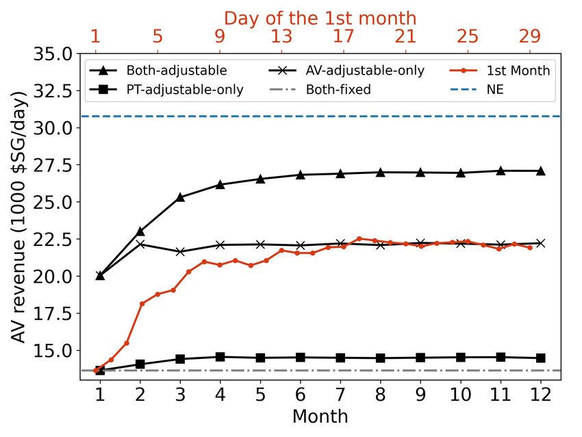
(Fagnant and Kockelman, 2015), land use patterns (Koh and Wich, 2012), and road safety (Zhang et al.,
2016). As a critical component of urban transportation, public transit (PT) systems cannot avoid the impact
of AV. Due to the uncertainty of how the AV systems may evolve, many different scenarios of AV–PT
interactions have been proposed (Lazarus et al., 2018). Some studies argue that AVs will compete with the
PT systems (Levin and Boyles, 2015; Chen and Kockelman, 2016) or even replace them (Mendes et al.,
2017), while others are optimistic about the AV–PT integration, stating that they could be complementary to
each other (Lu et al., 2017; Wen et al., 2018).
     AV–PT integration has been studied under various operation and regulation scenarios. Salazar et al.
(2018) proposed a tolling scheme for an AV–PT intermodal system, which shows a significant reduction
in travel time, cost, and emissions compared to a single-mode scenario. Shen et al. (2018) and Wen et al.
(2018) envisioned the transit-oriented autonomous mobility-on-demand (AMoD) systems in Singapore and
London. However, the integrated AV–PT system requires significant regulatory interventions and operators
willingness to collaborate. In many contexts, the AV and PT operators will likely behave as competitors by
default. There are fewer studies on the competitive perspective of the relationship. Some prior research only
evaluated the effect of AV on PT but did not specify the competition mechanisms between them (Levin and
Boyles, 2015; Childress et al., 2015). Recently agent-based models (ABM) have been used to investigate
the competition. Both Liu et al. (2017) and Mendes et al. (2017) argued that traditional PT services may
not survive once the shared AV services become available; but they only considered the AV–PT competition
to be a single-shot process—how PT systems are affected when AV is introduced—rather than a repeated
process where both AV and PT can adjust their supplies dynamically during the competition.
     Our study examines the competitive perspective where both AV and PT operators are profit-oriented with
dynamic adjustable supply strategies. In classic economics, market competition can ideally lead to optimal
resource allocation. However, due to the common market failures in the transportation industry, regulations
are often imposed, or even a certain level of cooperation is mandated. We examine five regulation scenarios
(Table 1), which can be categorized by a two by two matrix regarding whether the AV operator is allowed to
change the fleet size and whether the PT operator is allowed to adjust headway. The impact of different PT
subsidies on the competition results of five scenarios is also evaluated. Other important regulation aspects,
such as service fare, pricing, and bus routes, are assumed to be fixed across all five scenarios.
                                 Table 1: Regulation scenarios examined in this paper

                                                                    PT supply
                          Regulation Scenarios
                                                          Fixed                 Adjustable
                                       Fixed          Both-fixed           PT-adjustable-only
                        AV supply
                                     Adjustable    AV-adjustable-only     Both-adjustable / NE

    • The “Both-fixed” scenario corresponds to a fully-regulated transportation market without competition
      (Shen et al., 2018). The supplies, fare structure, route network, and service areas are all set by transport
      authorities. Neither AV nor PT is not allowed to change their supply.
    • The “AV-adjustable-only” scenario allows AV to adjust supplies but with all other operation parameters
      (e.g. price) fixed. The PT operators cannot adjust service headways. This is close to the situation
      where the ride-sourcing services, such as Uber and Lyft, are operated independently from transit
      agencies.
    • The “PT-adjustable-only” scenario allows PT operators to adjust the service headways to maximize
      their profits. This gives the PT operators even more flexibility than the well-known ”Scandinavian” or
      ”London” organization models (Costa, 1996; van de Velde, 1999), where the transport authority sets
      the service goals and then contracts out transit services to private operators.

                                                          2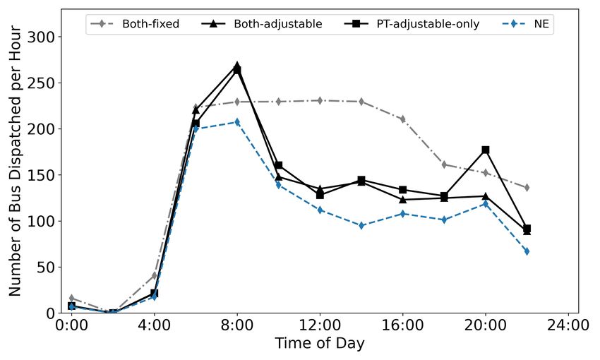
• When both operators are allowed to adjust supplies, we have two different scenarios: “Both-adjustable”
      and “Nash Equilibrium” (NE). These two scenarios have the weakest regulation compared to the
      other three and are close to the situation in the UK (except for Greater London) (Wilson, 1991),
      where all operators are private and compete against each other. The difference between these two
      scenarios can be looked at from two aspects: 1) Conceptually, the both-adjustable scenario can be seen
      as a “constrained” competition while NE “non-constrained” competition. Both-adjustable scenario
      allows both PT and AV to adjust supplies according to a “constrained” profit-maximization strategy.
      Specifically, due to incomplete market information and the regulation from the government, the supply
      updating at each step may not be optimal (see Section 3.5 for details). Therefore, the system may not
      converge to the NE. However, for the NE scenario, we use the iterated best response (IBR) algorithm
      to find the NE. A NE is a profile of strategies such that each strategy is the best response to the
      rest of the profile. That is, each agent maximizes its own utility given the strategies played by the
      others. The supply updating at each iteration is the agent’s best response to the environment and the
      competitor’s strategy. 2) Algorithmically, since AV and PT’s actions at each step are not optimal in the
      both-adjustable scenario, the both-adjustable scenario can be seen as a premature convergence result
      of IBF due to the non-optimal responses of competitors.

    We selected the first-mile connection to the subway station (Lesh, 2013) in Tampines, Singapore as the
study area where there are multiple bus feeder services, and implemented an agent-based model to simulate
the competition process between AV and PT including a heuristic algorithm to update the AV and PT supplies
based on the operators’ historical actions and profits. We evaluated the competition between AV and PT as
well as the system performance from the standpoints of four stakeholders—the AV operator, the PT operator,
passengers, and the transport authority.
    The remainder of this paper is organized as follows. Section 2 reviews the literature and identifies the
research gaps. Section 3 introduces system design, agent behavior, and performance metrics. Section 4
presents the results, and Section 5 concludes the paper.

2. Literature Review

AV is expected to reshape the future transportation system from different perspectives. Many advantages of
AV, such as absolute compliance, expanded service hours, reduced labor forces, and human errors make it an
efficient mode of urban transportation, which enables the reduction of operating costs and serves the travel
demand for fewer fleet sizes (Fernández L. et al., 2008; Alonso-Mora et al., 2017; Spieser et al., 2014).
    Given the promising application of AV, recent studies have examined the impact of AV in different
aspects, such as traffic flow (Talebpour and Mahmassani, 2016), road congestion (Fagnant et al., 2015),
land use (Koh and Wich, 2012), and road safety (Zhang et al., 2016). Talebpour and Mahmassani (2016)
used a micro-simulation model to evaluate the impact of connected and autonomous vehicles on traffic flow
and showed that AV can improve string stability and help prevent shockwave formation and propagation.
Azevedo et al. (2016) applied an integrated agent-based micro-simulation model to design and evaluate the
impact of AV on people’s travel behavior. They found that the new AV technology can change people’s
travel patterns, in terms of mode shares, route choices, and activity destinations. Fagnant and Kockelman
(2014) indicated that each shared AV can replace approximately 11 conventional vehicles, but it adds up to
10% more travel distance than comparable non-shared AV trips. There are also empirical studies in Lisbon
(Martinez and Viegas, 2017), Toronto (Kloostra and Roorda, 2019), and New Jersey (Zhu and Kornhauser,
2017), which reveal that the AV technology can reduce traveled vehicle kilometers and emissions (Martinez
and Viegas, 2017), average travel time (Kloostra and Roorda, 2019), and the number of vehicles on the road
(Martinez and Viegas, 2017).

                                                      3
However, despite the large volume of recent research on the impact of AV, research focusing on the
AV–PT interaction is limited. Two major relationships between AV and PT have been discussed in the
literature.
     First, AV and PT can be complementary and integrated. AV and PT can be cooperative in a way that AV
is integrated as a part of the PT system for social welfare. In line with this assumption, Ruch et al. (2018)
used a simulation model to analyze whether AV can substitute the rural PT lines. They found such a service
can operate at a lower cost and with a higher service level when the PT lines are short and are underutilized.
Similarly, Shen et al. (2018) designed an AV–PT integration system with AMoD as an alternative to low-
demand bus routes, which showed that the integrated system has the potential to enhance service quality,
occupying fewer road resources and being financially sustainable. Another cooperative scenario is the multi-
modality between AV and PT. For example, Yap et al. (2016) conducted a stated preference survey to analyze
the use of automated vehicles as the egress mode of train trips. They found that AV is a good alternative for
first-class train passengers. Liang et al. (2016) used an integer programming model to study AV as a last-mile
connection to train trips, which showed that using automated taxis can reduce the pick-up cost and improve
profits. Vakayil et al. (2017) proposed a hybrid transit system where AMoD serves as the first- and last-mile
feeder for the subway. The results show that an integrated system can provide up to 50% reduction in total
vehicle miles traveled. These studies provide sufficient analysis toward the AV–PT integration relationship.
The co-operation strategies for AV and PT are also designed (Salazar et al., 2018).
     Second, AV can be competitive with traditional PT when AV is operated privately and competes for
market share and profit. The analysis of this scenario is very limited. Using a multiclass four-step model,
Levin and Boyles (2015) found that the transit ridership will decrease when AV is introduced. Similarly,
Childress et al. (2015) used an activity-based model to evaluate the impact of AV, which revealed a reduction
in PT’s mode share. Liu et al. (2017) simulated the impact of shared AV based on a case study in Austin,
Texas, and showed that conventional PT services may not survive once the shared AV services become
available. Mendes et al. (2017) developed an event-based simulation model to compare the shared AV
services with the proposed light rail services in New York City and found that AV is more cost-efficient in
providing the same level of service. Basu et al. (2018) applied an activity-driven agent-based simulation
approach to test the impact of AV on mass transit and found that AMoD indirectly acts as a replacement to
mass transit.
     Understanding how AV competes with PT is critical for managing future PT services and developing
sound intervention on the private transportation market. However, existing studies addressing the AV–PT
competition focused on the static interaction process, i.e., they only considered what will happen when AV is
introduced as a one-shot game. However, as competitors, it is highly likely that AV and PT will dynamically
adjust the operation strategies in the market as repeated games. These interactive dynamics have not been
considered in the literature. Moreover, most existing studies only evaluate the AV’s impact on the mode share
of PT, without a comprehensive assessment of the cost and benefit of different stakeholders in the system,
including operators, passengers, and transport authorities.
     In this study, we used an agent-based model to simulate the competition between AV and PT, with
both parties trying to increase their profits. We also comprehensively evaluated the system from different
stakeholders’ perspectives, including the financial conditions, the level of service, vehicle kilometer traveled
(VKT), and transport efficiency, aiming to fill the research gap in the literature.

3. System design

We used the Tampines Planning Area in Singapore as the study area to apply our AV–PT competition
model. We focused on the first-mile trips heading to the Tampines Mass Rapid Transit (MRT) station from
surrounding residential blocks. Walking and buses are currently the dominant modes for first-mile trips (Mo
et al., 2018). Bus service in Singapore is highly regulated by the Land Transport Authority (LTA), which

                                                       4
is responsible for its fare structure and route design. The LTA contracts out bus services to different bus
operators on a five-year basis. Note that as walk and bus are currently dominant travel modes, AV may have
a great potential to increase its ridership and compete with PT in this first-mile market.

3.1. Basic assumptions
Based on the characteristics and the operational structure of the Singapore transport system, we make the
following assumptions for the AV–PT competition model.

  (a) System-level

         • Travel mode: Before AV entering the market, walking, bus, and ride-hailing are the only travel
           modes available for the first-mile trips. After AV emerges, ride-hailing will be replaced by the
           AMoD. This assumption is based on the Singapore autonomous vehicle initiative policies (Land
           Transport Authority, 2017).
         • Traffic conditions: We perform a mesoscopic simulation; microscopic features such as signal
           system and driving behavior are not considered in this study. As AVs and buses in the first-mile
           market only account for a small proportion of traffic flows on roads, time-dependent exogenous
           congestion is considered. The speeds of AVs and buses on each road for different times of day
           are pre-obtained from the Google Map API.
         • Demand and supply: The spatial and temporal distributions of travel demand are assumed to be
           fixed for all simulated days. The supply of AV and PT can be adjusted for competition. The fixed
           demand assumption holds when the residential population and infrastructures do not change
           substantially in an area (especially within a short-time period). It can reflect the early stage of
           the market when AV is introduced.
         • Information: The AMoD and PT’s supply information is complete and in real-time for passengers’
           mode choice decisions.

  (b) Agent-level

         • Ownership: PT and AMoD are both operated by private enterprises but under government
           regulation, i.e., they are in a constrained competition (but NE scenario can be seen as an
           unconstrained competition).
         • Objective: PT and AMoD are able to adjust their supply to improve their profits.
         • Fare: PT and AMoD’s fare structures are fixed by the government and cannot be changed.
         • Operating cost and subsidies: PT and AMoD’s operating cost is proportional to their fleet size
           and driving distance. There is no operation subsidy for PT based on the current Singapore policy
           (Gopinath and Kuang, 2018). However, we test several hypothetical scenarios with different
           levels of subsidies to enrich the discussion. Details are shown in Section 3.7 and 4.5.
         • Constraints: PT has a lower bound and an upper bound for the bus headway. AMoD has an upper
           bound for the maximum fleet size.
         • Dynamic intraday supply: AMoD and PT’s supply can be different in different time periods in a
           day.
         • Supply updating frequency: AMoD can update the next day’s supply strategy at the end of each
           day. PT can only update its supply strategy after a sufficiently long time (30 days in this study;
           more discussion in Section 3.5). For the NE scenario, there is no definition of supply updating
           frequency (see Section 3.6 for details).

                                                     5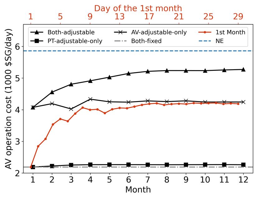
To summarize, the AMoD updates the supply daily by adjusting the vehicle fleet size in each time interval
of the next day and PT adjusts its supply by changing the headway for each bus route in different time intervals
in a month.
     Price adjustment is also a common practice to increase profit in market competition. However, to isolate
the impact of the supply change, we only focus on supply in this study, assuming that the prices are fixed for
both PT and AMoD. Moreover, given the price regulation history of the LTA, it is very likely that the AMoD
will be regulated on the fare structure to avoid price wars (Singapore Public Transport Council, 2019). Future
research can explore a combined model incorporating supply change and pricing.

3.2. Study area
Tampines is a 6.86-km2 mixed residential and commercial area located in eastern Singapore (Figure 1a). It is
centered around the Tampines MRT station, which is one of the busiest MRT stations in Singapore (Housing
& Development Board, 2015). Fifty-one bus stops serve Tampines, with 26 bus routes connecting to the
MRT station. Three of them are dedicated feeder routes to the subway. The other 23 are passing-by routes.
All 26 routes are included in the simulation model. We chose Tampines for the case study to illustrate the
feasibility of our model because 1) it possesses a significant first-mile demand to the MRT station, and 2) it
houses a large volume of bus supply, which provides a non-trivial testbed for competition analysis.
     The first-mile travel demand was obtained from the transit smart card data. The dataset covers all PT
trips in August 2014. A normal workday in August 2014 was selected as the study date. Since the smart
card data in Singapore include both tap-ins and tap-outs, the accurate date and time of each entry and exit
activity are recorded, as well as the boarding and alighting stops/stations, which allows us to extract complete
first-mile demand by counting passengers who tap into the Tampines MRT station. The temporal distribution
of first-mile travel demand on the study day is shown in Figure 1b. A total of 51,850 passengers entered the
Tampines MRT station on the study day.

3.3. Stakeholders and system evaluation
We evaluated the interests of multiple stakeholders in the AV–PT competition. Table 2 identifies four
key stakeholders (passengers, AMoD operators, PT operators, and transport authority) and their evaluation
indicators.
    The main interests of passengers are the level-of-service and modal choice. The level-of-service indicators
include travel cost, total travel time, waiting time, and generalized travel cost —calculated as the sum of
walking time, waiting time, and riding time multiplied by the corresponding value of time (VOT). It is a
comprehensive value that incorporates both travel time and travel costs. The VOTs were derived from the
estimated choice model in Table D.1. In terms of modal choice, the number of travelers choosing walking,
buses, and AV was recorded, respectively.
    The interests of AMoD and PT operators, based on our profit-orientation assumption, are financial
viability and supply. The financial viability indicators include operating cost, revenue, profit, and market
share, while the supply indicates the number of AV/bus supplied.
    For the transport authority, efficiency and vehicle kilometer traveled were considered. The average load
per vehicle is one of the indicators of transport efficiency, which is calculated using the total passenger travel
distance divided by the total vehicle travel distance. We considered the vehicle kilometers traveled (VKT)
and total passenger car equivalent (PCE). The unit PCE for a bus was set as 3.5 in this study (Ahuja, 2007).
    These indicators were recorded in the simulation process, which shows the entire changing profile during
the competition between AV and PT. The time of the day distribution of some indicators was also recorded.

3.4. Agent behavior
The overall simulation system is composed of three main types of agents: buses, AMoD vehicles, and
passengers. The PT system is derived from Shen et al. (2018)’s study, which has been calibrated and

                                                       6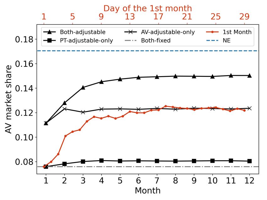
(a) Study area

                      (b) Time-of-day distribution of first-mile demand to Tampines MRT station

                                          Figure 1: Study area and demand

validated with real-world data. Here we give an overview of the behavior of the agents, with detailed
formulation given in Appendix A.

   • Passengers’ mode choices are based on mixed logit models using trip-specific variables (waiting
     time, in-vehicle time, and monetary cost) and individual-specific variables (household income); if a
     passenger chooses the bus or AMoD, a maximum waiting time is considered to avoid a shortage of
     services. The passenger changes to other modes if the maximum waiting time is reached
   • AMoD dispatching is based on the first-come-first-serve principle upon passengers’ requests. The
     vehicles follow the shortest paths from pick-up locations to the MRT station. When there is no empty
     vehicle available, the dispatching center will then look for vehicles with passengers who agree to share
     their trips. Every day, the AMoD operator updates the fleet size of each time period of the day to
     increase its profit.
   • Buses follow the existing routes given by the LTA. Each month, the operator for each bus route
     independently optimizes its profit by changing the headway of each time period of the day.

                                                         7
Table 2: Evaluated indicators of stakeholders

                  Stakeholder                Interests                          Indicators
                                                                                 Travel cost
                                                                              Total travel time
                                          Level of service
                                                                               Waiting time
                   Passengers                                             Generalized travel cost
                                                                             Walking demand
                                           Mode choice                          Bus demand
                                                                                AV demand
                                                                               Operation cost
                                                                                  Revenue
                                        Financial viability
                AMoD Operators                                                     Profit
                                                                               Market share
                                              Supply              Average number of AV provided per hour
                                                                               Operation cost
                                                                                  Revenue
                                        Financial viability
                  PT Operators                                                     Profit
                                                                               Market share
                                              Supply                 Number of bus dispatched per day
                                                                        AV average load per vehicle
                                        Transport efficiency
                                                                        Bus average load per vehicle
               Transport Authority                                                AV VKT
                                     Vehicle kilometer traveled                  Bus VKT
                                                                          Total PCE (AV and PT)

3.5. Competition process
An agent-based simulation model is used to perform the AV PT competition process. There are four sets of
input variables/parameters: simulation setting parameters θ, initial supply strategies of the bus S (0)
                                                                                                     B , initial
                               (0)
supply strategies of AMoD S A , and the first-mile demand D. The detailed notations and values used are
given in Table 3. The values of these constants were chosen based on the Singapore context (details in
Appendix A).
    The supply, profit, and supply changing units are all time-specific for AV, which means that for different
days and different time periods they may have different values. For buses, these variables are time- and route-
specific. The pseudo-code for the competition process (both-adjustable scenario) is shown in Algorithm
1.
    As shown in Algorithm 1, the overall framework aims to simulate the interaction between AV and PT
over time period T. One-Day-Sim is a pseudo function of running the simulation for a single day given the
supply, demand, and θ, which is considered as the engine of the simulation model. In this function, each
agent will follow the behaviors mentioned in Appendix A.
    The profits of AMoD and PT can be obtained after running this function. The profit, supply, and supply
change unit are then used as the input of function SupplyUpdate (shown in Algorithm 2), deriving the
updated supply strategies and new supply change units for AV and PT. Since we assume that the AV supply
updating frequency is daily, this function is executed for AV every day, while it is executed for PT every NB
days, considering the limited flexibility of PT planning.
    In practice, the PT schedules do not adjust frequently. A reasonable period should be more than three
to six months, which allows the transit operators to notify the passengers and gives people enough time to
adapt to the new schedule. Based on our numerical test, however, given a specific bus schedule, the system
will stabilize in one or two weeks when only the AMoD updates its supply. Therefore, any values of NB
that are greater than two weeks are equivalent because the system state will not change after two weeks. In
this study, NB = 30 days was used to simulate the long-period updating frequency of the bus. The system
evaluation indicators (Table 2) were recorded during the simulation and returned at the end of the model.

                                                              8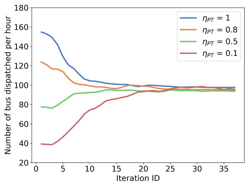
Table 3: Notations and values of system parameters

     Categories                                   Parameters/Variables                                            Value
                                                Duration of simulation (T)                                      365 days
                                         Supply changing unit reduced factor (γ)                                   0.75
                                              Passenger choice lag factor (α)                                       0.5
                                         Passenger mode choice parameters (β)                                See Table D.1
                                          Passenger maximum AV waiting time                                      10 min
                                          Passenger maximum bus waiting time                                     30 min
                                          Passenger ride-sharing-agreement rate                                    50%
                                               AV supply time interval (i A)                                     1 hour
                                           AV supply updating frequency (N A)                                     1 day
Simulation setting                                AV fixed operation cost                                   4 SGD/hour·veh
parameters (θ)                                  AV variable operation cost                                   0.12 SGD/km
                                               AV base distance of fare (db )                                     1 km
                                                     AV base fare ( fb )                                        3.4 SGD
                                                AV distance-based fare ( f )                               0.22 SGD/400 m
                                            AV detour discount rate of fare (λ)                                      2
                                               AV supply lower bound (S AL )                                         0
                                               AV supply upper bound (SU     A)                                    150
                                          AV initial supply changing unit (C Aini )                            10 vehicles
                                               Bus supply time interval (iB )                                    2 hour
                                           Bus supply updating frequency (NB )                                   30 days
                                                    Bus operation cost                                       2.71 SGD/km
                                                       Bus dwell time                                             30 sec
                                                           Bus fare                                          0.77 SGD/trip
                                             Bus headway upper bound (SU      B)                                2100 sec
                                              Bus headway lower bound (SBL )                                     210 sec
                                        Bus initial headway changing unit (CBini )                                3 min
                                 Bus headway of route l in time interval t on day d (SBl,t,d )                Intermediate
    Bus supply S B                Bus headway arrangement on day d (S (d)              l,t,d
                                                                             B = [SB ]l,t )                   Intermediate
                                         Bus initial headway arrangement (S (0)    B )                     See Appendix A.3
                                 Number of AV supplied in time interval t on day d (S t,d      A )            Intermediate
    AV supply S A                     AV supply strategies on day d (S (d) A  =   [S t,d
                                                                                     A t ] )                  Intermediate
                                             AV initial supply strategies (S (0)
                                                                               A  )                        See Appendix A.2
     Demand D                                  Demand of first-mile trips D                                  See Figure 1b
                                      AMoD profit in time interval t on day d (pt,d     A )                   Intermediate
                                                                          (d)       t,d
                                      AMoD profit vector on day d ( p A = [p A ]t )                           Intermediate
                                AV supply changing unit in time interval t for day d (C At,d )                Intermediate
     Supporting                 AV supply changing unit vector on day d (C (d)               t,d
                                                                                  A = [C A ]t )               Intermediate
     variables                    Bus profit of route l in time interval t on day d (pl,t,d B )               Intermediate
                                                                     (d)      l,t,d
                                        Bus profit vector day d ( p B = [pB ]l,t )                            Intermediate
                          Bus headway changing unit of route l in time interval t for day d (CBl,t,d )        Intermediate
                                                                                  (d)
                              Bus headway changing unit vector on day d (C B           = [CBl,t,d ]l,t )      Intermediate
*   Values of “intermediate” means the intermediate variables in the model.

                                                                     9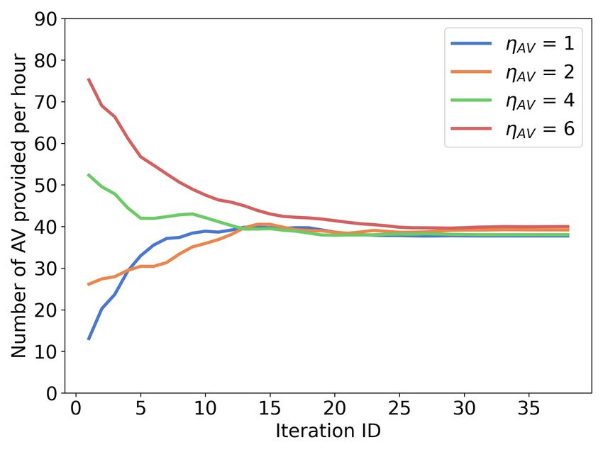
Algorithm 1 AV-PT competition (both-adjustable scenario)
 1:   procedure AV-PT competition(θ, S (0)                    (0)
                                                        B , S A , D)
 2:      Initialize p (0)             (0)         (1)      (0)
                        A = 0, p B = 0, S A = S A , S B = S B
                                                                  (1)      (0)

 3:      Initialize C (1)
                        A = C A , C B = CB
                                  ini     (1)      ini

 4:      Let day counter d = 0
 5:      while d < T do
 6:          d = d+1
 7:           p (d)    (d)                            (d) (d)
                A , p B = One-Day-Sim(S B , S A , D | θ)
 8:          S (d+1)
                A     , C (d+1)
                           A      = SupplyUpdate( p (d)      A , pA
                                                                    (d−1) (d)
                                                                         , S A , C (d)
                                                                                   A )
 9:          if d mod NB == 0 then
10:                S (d+1)
                     B      , C (d+1)
                                B       = SupplyUpdate( p (d)     B , pB
                                                                        (d−N B ) (d)
                                                                                , S B , C (d)
                                                                                          B )
                                   (d)
11:                Initialize C A = C A       ini

12:          else
13:                S (d+1)
                     B       = S (d)
                                  B
14:                C (d+1)
                      B       =  C (d)
                                   B
15:       return the system evaluation indicators (Table 2)

     It is worth noting that Algorithm 1 is designed for the both-adjustable scenario. When AV or PT are
not allowed to update their supplies, Algorithm 1 is revised with the corresponding supply updating steps
removed. The IBR algorithm for estimating NE (i.e. the NE scenario) is different from Algorithm 1 and thus
elaborated in Section 3.6.
     In terms of supply updates, we proposed a heuristic algorithm, which applied to both AMoD and PT.
Specifically, for AMoD, at the beginning of a day, the algorithm determines the AV fleet size for each hour
in the day. For PT, at the beginning of a month, the algorithm determines the PT headway for each route and
each hour for all days in the month.
     In this study, we assume the profits across different time periods and routes are independent, which leads
to a simple univariate optimization problem for each route and time period combination. For example, pl,t,d  B ,
the profit of bus route l at time interval t on day d only depends on the headway of route l at time interval t
on day d. Then, we can adjust the supply of l in the same time interval SBl,t,d to improve the corresponding
profit as a single-variable optimization problem. Similarly for AMoD, if the profit pt,d                   t,d−1
                                                                                        A is greater than p A    ,
                              t,d−1
the last change in supply C A       will lead to the profit increase. Thereupon, we can continue increasing the
fleet size of the same time period on the next day.
     If the change in profits between two supply strategies becomes sufficiently small (the threshold was set
to be 5%), we reduce the size of the changing unit by γ (i.e., C t,d+1 = γ · C t,d+1 ). This setting ensures the
convergence of the results.
     We acknowledge that the heuristic algorithm is a simplification for the profit maximization problem
because the profits of different time periods and routes are likely to be dependent on each other, especially
when the routes have overlapping stations. Nonetheless, we apply this simplified algorithm for the following
reasons: 1) The concept of this algorithm is in line with the reality, where information is incomplete and
every adjustment is a trial of a new supply strategy based on previous experience; 2) This heuristic algorithm
indeed yields an improved profit, which satisfies the initial purpose of adjusting the supply by the operators;
and 3) Capturing the dependency will require a much more complicated optimization problem, which we
suggest as a future research topic.
     We implemented the model on AnyLogic 8.1. The simulation is executed for T = 365 days to ensure
that the competition process converges.

                                                                   10
Algorithm 2 Supply updating
1: procedure SupplyUpdate( p (d) , p (d−N ) , S (d) , C (d) )
2: Let the index of elements in p (d) , p (d−N ) , S (d) and C (d) correspond with each other. (i.e., the k-th
element of p (d) , p (d−N ) , S (d) and C (d) represents the information of same time interval and same route.)
3: Initialize k = 0
4: while k < (length of p (d) ) do
5: k = k +1
6: Let pk,d , pk,d−N , S k,d C k,d be the k-th element in p (d) , p (d−N ) , S (d) and C (d) , respectively.
7: if pk,d > pk,d−N then
8: C k,d+1 = C k,d
9: else
10: C k,d+1 = −C k,d
11: S k,d+1 = S k,d + C k,d+1
12: if S k,d+1 violates the upper or lower bound constraints then
13: Set S k,d+1 equal to the upper or lower bound
14: C k,d+1 = γ · C k,d+1
15: if the difference between pk,d and pk,d−N is small enough then:
16: C k,d+1 = γ · C k,d+1
(d+1)
17: Let S = [S (k,d+1) ]k and C (d+1) = [C (k,d+1) ]k
18: return S (d+1) , C (d+1)
3.6. Iterated best response for solving Nash Equilibrium
For a competition game, one of the most important tasks is to find the NE if it exists. In this study, as
the environment (e.g., daily demand patterns and infrastructure layouts) does not evolve over time, the
competition between AV and PT with adjustable supplies can be seen as a static game1 . One way to solve
the pure NE in a static game is the IBR algorithm. In the IBR, each player in the game chooses strategies
iteratively, and every action they have selected is the best response (or one of the best responses) to the other
players’ strategies (Nash et al., 1950). The success of IBR depends on the context of a game. It has been
shown that IBR can always converge to a pure NE for any finite potential game, i.e., games in which the
payoffs of all players to change their strategies can be expressed using a single global function called the
potential function (Monderer and Shapley, 1996). There are also some counterexamples of coordination
games where IBR does not converge. However, in this study, it is hard to provide a theoretical analysis of the
pure NE existence and the performance of IBR because the payoff (i.e. profit) of each player is calculated
from an agent-based simulation without analytical forms. Therefore, we first implement the IBR and discuss
its convergence with numerical examples in Appendix B.
The details of the IBR algorithm is shown in Algorithm 3 and 4, where I is the maximum number of
iterations and ϵ¯ is a predetermined threshold for the termination of the best response algorithm. The best
response at each iteration is solved by using the SupplyUpdate algorithm for a specific player many times
(while fixing the supply for another player) until the profit increment is small enough. Compared to the
both-adjustable scenario where SupplyUpdate is only implemented once per step, the supply strategies at
each iteration in the NE scenario is closer to the optimal. Therefore, both-adjustable scenario can be seen as
a premature convergence result of IBF due to non-optimal responses of PT. However, we have to admit that
Algorithm 4 is still a heuristic way to find the best response, in which the results may still not be optimal.
1 Note that though this is a static game, the competition can still be seen as a dynamic process, where AV and PT react to each
other’s strategies as opposed to previous studies without supply updating.
11Algorithm 4 can be seen as uni-variate adaptive step size random searching, which is capable of finding
an optimal solution for convex function but may converge to a local optimum for a non-convex function
(Schumer and Steiglitz, 1968). As the profit functions of AV and PT have no analytical form, we cannot
provide more theoretical analysis here. In Appendix B, we test the convergence results of the proposed
IBR with respect to different initial AV and PT supplies numerically. And it is found that the system can
always converge to a similar supply level (which can be seen as an approximated pure NE). This validates
the effectiveness of the IBR algorithm proposed in this study.
Algorithm 3 Iterated best response for solving the Nash Equilibrium
1: procedure IBR(θ, S (0) (0)
B , S A , D)
2: Initialize p (1) (1) (1) (0)
A = 0, p B = 0, S A = S A , S B = S B
(1) (0)
3: Initialize C (1) ini (1)
A = C A , C B = CB
ini
4: Let iteration ID i = 0
5: while i < I do
6: i =i+1
7: S (i+1)
A , SB
(i+1)
=BestResponse(S (i) (i) (i) (i)
A , S B , C A , C B , θ, D)
8: p (i+1)
A , pB
(i+1)
= One-Day-Sim(S (i+1) (i+1)
B , S A , D | θ)
9: for k= 1:length of p (i+1) A do
10: if the difference between p(k,i+1) A and p(k,i)
A is small enough then:
k,i+1 k,i
11: CA = γ · CA
12: for k= 1:length of p (i+1)
B do
13: if the difference between p(k,i+1)
B and p(k,i)
B is small enough then:
14: CBk,i+1 = γ · CBk,i
15: return the system evaluation indicators (Table 2)
3.7. Scenarios settings
There is a rich space for all the value combinations of θ, as shown in Table 3. Each value combination
represents a distinct assumption of competition markets—some are realistic and some are not. It is not the
focus of this study to systematically explore all possible scenarios. From the market organization perspective,
we only focus on the five regulation scenarios introduced in Section 1 (Table 1).
In addition, we conduct another set of experiments with respect to different subsidy levels provided to the
PT. Specifically, in the case study (Section 4.5), we test two different subsidy schemes: demand-based and
supply-based. The demand-based subsidy is provided to PT operators on a per passenger served basis, while
supply-based subsidy on a bus kilometer operated basis. The sensitivity analysis for subsidy can be seen from
two aspects. First, it reflects different schemes of revenue and cost calculation. Demand-based subsidies can
be seen as the sensitivity analysis for revenue calculation while supply-based for cost calculation. Second,
subsidies can be seen as positive externalities of passengers using PT. From this angle, PT’s objective is
not only profit but also social welfare. Providing subsidies to PT can be seen as a way for the government
to internalize the positive externalities. Note that we approximate the change of social welfare using the
increase or reduction of government subsidy in this article, while acknowledging that social welfare involves
a broader category of considerations, including equity, caring for disadvantaged social groups, fostering
social interaction, etc. We leave the broader discussion of the impact of public transportation on social
welfare for future research.
12Algorithm 4 Best response
1: procedure BestResponse(S A, S B , C A, C B , θ, D)
2: Initialize p (0) (1) (1)
A = 0, S A = S A, C A = C A
3: Let day counter d = 0
4: while ϵ > ϵ¯ do ▷ Find the best response for AV
5: d = d+1
6: p (d) (d) (d)
A , p B = One-Day-Sim(S B, S A , D | θ)
7: S (d+1) , C (d+1) = SupplyUpdate( p (d), p (d−1), S (d) (d)
A , CA )
A
∑ A (k,d) ∑ (k,d−1) ∑ A(k,d−1) A
8: ϵ = |( k p A − k p A )/ k p A |
(d+1)
9: A = SA
S BR
10: Initialize p (0) (1) (1)
B = 0, S B = S B , C B = C B
11: Let day counter d ′ = 0
12: while ϵ > ϵ¯ do ▷ Find the best response for PT
13: d ′ =′ d ′ +′ 1 ′)
14: p (d ) (d )
A ′ , pB = One-Day-Sim(S (dB , S BR
A , D | θ)
(d +1) ′
(d +1) ′) ′ −1) ′) ′)
15: SB , CB = SupplyUpdate( p (d , p (d , S (d , C (d )
∑ (k,d′) ∑ (k,d′−1) ∑ (k,d′−1) B B B B
16: ϵ = |( k pB − k pB )/ k pB |
(d′ +1)
SB = SB
BR
17: return S BR A , SB
BR
4. Results and discussion
4.1. PT perspective
Figure 2 presents the indicators of interest for PT operators, including revenues, operating costs, profits,
supplies, and market shares. Each point in the graph represents the average value of the corresponding
month (same for all the following graphs).
The final PT profit of the PT-adjustable-only scenario is higher than those in all other scenarios because
there is no AV competition in this scenario, and is the lowest in the AV-adjustable-only scenario, reflecting
the competition of AV reducing the profit of PT. Both the revenue and operating cost of PT decrease over
the simulation period, but the operating cost shows a sharper reduction. Both the revenue and the cost of the
NE scenario are the lowest among all scenarios, indicating that the market share of buses is reduced in this
scenario. However, in terms of PT profit, the NE scenario is roughly at the same level as the both-adjustable
scenario, which means that the bus supply is similarly optimized towards profit in the two scenarios.
The number of buses dispatched per day and PT’s market share (Figure 2d and 2e) have a similar declining
trend. Since buses do not change supply in AV-adjustable-only and both-fixed scenarios, the supply curves
of these two scenarios are flat. The bus supply and market share decrease with AV competition and reach
the lowest levels in the NE scenario.
13(a) PT revenue (b) PT operation cost (c) PT profit
(d) PT supply (e) PT market share
Figure 2: Indicators of PT’s interest over the simulation process
One important observation is the additive effect of bus and AV supply adjustments. Take the bus market
share as an example. The curve of PT-adjustable-only scenario roughly represents how the PT operator
gradually "gives up" the unprofitable market share. The AV-adjustable-only curve shows how much market
share is grabbed by AV (i.e. the impact from AV supply adjustment). The both-adjustable scenario shows
the additive effect of two, which is nearly the sum of the two reductions. Moreover, the NE scenario has the
lowest PT market share among all, indicating a more "aggressive" bus supply optimization strategy. Later
results suggest that although the bus supply is significantly reduced in the NE scenario, the generalized travel
cost is reduced on average.
In addition to the total supply, we consider the change in temporal and spatial distributions of the supply
before and after adjustment (Figure 3). In the temporal dimension, the numbers of dispatched buses for
most time periods except for the morning peak (6:00–10:00) are reduced. This implies that the PT operator
concentrates the supplies to the morning and evening peak periods, which have higher demands and are more
profitable. In the spatial dimension, some routes (e.g., 29_1, 28_2) are allocated with higher frequencies,
while some routes (e.g., 291_2, 292_1) are adjusted to a lower service rate. The routes with increased and
reduced supplies are shown in Figure 3c and 3d, respectively. Overall, the increased-supply routes are short
and cost-efficient and they cross the residential areas and are directly connected to the MRT station. The
routes with decreased supply are long and sinuous and greater reductions in the operating cost are achieved by
decreasing the supply of these routes. Therefore, the change in the spatial distribution is related to an implicit
coordination within the bus routes (even if our algorithm does not consider the inter-route coordination). To
summarize, the PT operator reduces the supply for higher-cost routes and transfer the service to the lower-cost
routes, resulting in a more profitable operation scheme. On both the spatial and temporal distributions, the
NE scenario resembles the results of both adjustable, but with each route and time period slightly lower.
14(a) PT supply temporal distribution
(b) PT supply spatial distribution
(c) Routes with increased supply (NE) (d) Routes with reduced supply (NE)
Figure 3: Spatial and temporal distribution changes in PT supply. Note that both-fixed scenario represents the initial distribution
before the supply adjustment.
4.2. AMoD perspective
As Figure 4 shows, AMoDs revenue, operating cost, and profit increase rapidly at the beginning and then
stabilize. The AMoD operator provides more services to improve its profit in the competition. As shown in
Figure 4d and 4e, the AMoD’s supply and market share keep increasing during the first few months and then
become stable. The major change in the AMoD’s supply happens in the first month. When both AV and PT
can adjust—including the both-adjustable and NE scenarios—the profit of AV is higher. The NE scenario
can achieve the highest AV profit and the largest market share, and the both-adjustable scenario rank the
second. The bus supply adjustment not only improves the profit of the bus but also benefits that of AV. This
15is because the initial bus service is over-supplied for the first-mile market. When the bus operator is allowed
to adjust its supply, some of the yielded unprofitable travel demand is served by AV. This observation is in
line with the previous research on the AV–PT integration system (Shen et al., 2018). Therefore, when PT is
oversupplied, although we assume that AV and PT compete with each other, they still implicitly show some
extent of cooperative behavior, resulting in higher profits for both. However, this cooperative feature is only
manifested when the bus changes its supply. The AV supply adjustment only unilaterally benefits itself.
(a) AMoD revenue (b) AMoD operation cost (c) AMoD profit
(d) AMoD supply (e) AMoD share
Figure 4: Indicators of AMoD’s interest over the simulation process. The first-month curve (red, with upper x-axis) for the AV-
adjustable-only and both-adjustable scenarios are the same because the bus supplies stay the same, and AV does not change in the
other two scenarios. Therefore, only one curve is shown for the first month.
For the AMoD’s operating cost (Figure 4b), the value in the NE scenario is the highest, followed by the
both-adjustable and AV-adjustable-only scenarios. This corresponds to the supply levels shown in Figure
4d. We also observe the additive effect of supply adjustment on the AV profit and market share. Different
from the effect on bus supply, the two changes both benefit AV. Thus, the both-adjustable scenario has higher
profit and market share than the AV-adjustable-only and the PT-adjustable-only scenarios. The NE scenario
has the highest AV revenue, operation cost, and also the highest profit and market share among all scenarios.
Similar to our analysis for PT, we also examine the time-of-day distribution of the AMoD supply before
and after the adjustment. As shown in Figure 5, the final supply patterns of NE, both-adjustable and AV-
adjustable-only scenarios are similar. After 12 months of adjustment, the supply was re-distributed across
time. More supply was provided in the morning and evening peak hours, which is considered more profitable.
The supply in off-peak hours (e.g., 11:00–13:00) stayed the same or became even lower. These temporal
changes correspond to the demand distribution in Figure 1b.
4.3. Passenger perspective
Figure 6 plots the changes in the level-of-service indicators: travel cost, total travel time, waiting time, and
generalized cost. Passengers’ travel cost shows different patterns: it decreases in the PT-adjustable-only
16Figure 5: Time of day distribution of AV supply
scenario and increases in all other scenarios, although the magnitude of the changes is small. Because AV
is more expensive than PT, when AV starts to compete and serve more demand, the average travel cost will
increase. When there are only buses adjusting the supply, a greater number of people will switch to walking
and only a small proportion of people will convert to AV (Figure 7)—the average travel cost will decrease.
The NE scenario observes the highest average travel cost due to the highest market share of AV.
All scenarios show decreasing trends for the total travel time. In the PT-adjustable-only scenario,
passengers’ travel time and travel cost both decrease after the adjustment of the bus supply, which implies
absolute benefits to passengers. Conversely, in the both-adjustable and AV-adjustable-only scenarios, the
directions of the changes in the travel time and cost differ. To capture the combined effect of travel time and
travel cost, we calculated the generalized travel cost based on the method described in Section 3.3.
As shown in Figure 6d, passengers’ generalized travel cost decreases in all scenarios, among which the
NE scenario shows the largest decline and both-adjustable scenario ranks the second. The supply adjustment
of buses and AV not only benefits the operators but also the passengers. The major contributing factor to the
changes in generalized travel cost is the decrease in travel time.
Another important indicator for passengers is waiting time. In the PT-adjustable-only scenario, passen-
gers’ waiting time increases as a direct consequence of the reduction of the bus supply (Figure 6c). In the
AV-adjustable-only scenario, passengers’ waiting time decreases because of the increased AV supply. In the
both-adjustable scenario, we observe a combined effect of the two. The gap between the first month and
both-fixed scenario is caused by the significant increase in the AV supply in the first month. Starting from
the first month, passengers’ waiting time gradually increases because the effect of bus supply reduction starts
to manifest. Nonetheless, due to the opposite effect from the AV side, the increase in waiting time is not
as pronounced as in the PT-adjustable-only scenario. The converged waiting time is still shorter than the
both-fixed scenario. The NE scenario has a slightly higher waiting time than the both-fixed scenario.
17(a) Travel cost (b) Total travel time
(c) Waiting time (d) Generalized travel cost
Figure 6: Level of service change
Figure 7 shows the passenger mode choice: the demand for AV increases, the demand for buses decreases
and the demand for walking varies across scenarios. In the both-adjustable and PT-adjustable-only scenarios,
more people turn to walk due to the reduced bus supply, whereas in the AV-adjustable-only scenario, fewer
people walk because of the increased supply of AV.
In addition to the aggregate demand changes, we explore the attributes of the passengers who change
their mode choices, i.e. from bus to AV or walking. For illustration purposes, we only show the analysis for
the both-adjustable scenario. We examine two passenger attributes, the household income and the distance
from home to the MRT station. People who originally chose buses were set as the control group. People who
changed their travel modes from bus to AV or walking were set as the experimental group. Our purpose is
to test whether there is a statistically significant difference between the control groups and the experimental
groups in their household income and distance to the MRT station. Table 4 summarizes the results of the
two-sample Kolmogorov-Smirnov (KS) test. For household income, the attributes of the people who changed
their mode choice from bus to AV are significantly higher than those of the control group. Higher-income
people tend to change from bus to AV after a decline in the bus supply. However, for people who chose
walking, household income does not show a significant difference. In terms of the distance to the MRT
station, the results for both experimental groups are significantly different from those for the control group.
People who live near MRT stations tend to walk more, while people who live far from MRT stations tend to
convert to AV. This implies that the interaction of AV and PT may sharpen people’s travel mode choices and
increase the dependence on cars for people living far from subway stations.
18(a) AV demand (b) Bus demand (c) Walking demand
Figure 7: Change of passenger mode choices
Table 4: KS Test Results for the AV–PT Scenario
Attributes Groups Mean (Std.) KS Statistics p-values
Baseline 4760.3 (3689.5) N.A. N.A.
Household Income (SGD) Experiment (Bus to AV) 5134.9 (3697.0) 0.061 0.000*
Experiment (Bus to Walk) 4731.3 (3668.9) 0.008 0.795
Baseline 1065.0 (333.1) N.A. N.A.
Distance to MRT Station (m) Experiment (Bus to AV) 1112.7 (320.4) 0.064 0.000*
Experiment (Bus to Walk) 933.1 (313.5) 0.166 0.000*
- Control groups are set as reference, so they do not have KS statistics and p-value.
- The larger the KS Statistics, the greater the difference between the two groups.
- *: Significant at 99% confidence level.
4.4. Transport authority perspective
We consider efficiency and vehicle kilometers traveled from the transport authority perspective as shown.
In Figure 8a and 8b, the average load of AV slightly increases in the PT-adjustable-only scenario. However,
in the both-adjustable and AV-adjustable-only scenarios, the AV load decreases considerably in the first
month (the gap between the both-fixed scenario and the first month) and then stabilizes. This suggests that
to maximize profit, ride-sharing behavior is inhibited in the model. Since travel distance is usually short
in the first-mile scenarios, ride-sharing is less likely to happen or generate higher profits. Considering the
proposed price structure of AMoD, serving two passengers with two vehicles separately may yield more
profit. Therefore, although the AMoD operator earns more profit, the AV’s operating efficiency is lower.
In contrast to AV, the average bus load increases for the both-adjustable and PT-adjustable-only scenarios,
which means that after the competition, the buses are operated more efficiently, with not only higher profit,
but also higher average load.
The NE scenario observes relatively low AV average load, and relatively high bus average load, but stays
in the middle positions among all scenarios.
Overall, the VKT of AV increases, while the VKT of buses decreases, which is consistent with the change
in supply (Figure 8c-8e). Since the unit PCE for the bus is large, the shape of the total PCE is similar to that
of the bus VKT. The system total PCE decreases in the both-adjustable and PT-adjustable-only scenarios,
which means that the deregulation of the bus operator has the potential to reduce the environmental impacts.
When the bus system is not allowed to change its supply, the total PCE increases owing to the increase in the
VKT of AV. The NE scenario has the lowest bus VKT, relatively low VKT of AVs, and overall relatively low
total PCE.
19(a) AV average load (b) Bus average load
(c) AV VKT (d) Bus VKT (e) Total PCE (bus + AV)
Figure 8: Change of transport efficiency indicators
4.5. Sensitivity analysis on PT subsidies
In this section, we compare five scenarios of PT subsidies including demand-based subsidies (0, 1, and 2
SGD per passenger trip) and supply-based subsidies (0, 0.5, and 1 SGD per km operated). It turns out the
two subsidy regimes show largely similar results and therefore we focus on the demand-based subsidies in
this section and leave the discussion on the supply-based subsidies in Appendix C.
4.5.1. PT perspective
Figure 9 shows the results of PT’s profit, supply, and market share under three different demand-based
subsidies. As expected higher demand-based subsidies result in an increase in PT profit, supply and market
share because the PT operator earns more money per passenger and thus maintains higher supply and market
share. Critically the PT profit turns positive when the subsidy level is greater or equal to 1 SGD/passenger.
The PT supply and market share of AV-adjustable-only scenario are not affected by the PT subsidy. The
change patterns of PT-adjustable-only, both-adjustable, and NE scenarios are consistent and similar.
20(a) PT profit (b) PT supply (c) PT market share
Figure 9: Impact of demand-based subsidies on PT operators. All bars represent the converged values of the corresponding
scenarios.
4.5.2. AMoD perspective
As shown in Figure 10, AV’s profit, supply, and market share all decrease with the increased PT’s subsidy.
Those changes are more prominent in both-adjustable and NE scenarios. AV-adjustable-only scenario is not
affected because the updating of AV only depends on the environment and PT’s supply, which is fixed by
definition in this scenario. The impact on PT-adjustable-only scenario is negligible.
(a) AMoD profit (b) AMoD supply (c) AMoD market share
Figure 10: Impact of demand-based subsidies on AMoD operators
4.5.3. Passenger perspective
From the passenger’s perspective, we plot travel cost, travel time, waiting time, and generalized travel cost
averaged across all modes. For the travel costs (Figure 11a), we observe a slight decrease in both-adjustable
and NE scenarios, but a slight increase in the PT-adjustable-only scenario. In the both-adjustable and NE
scenarios, the subsidy allows PT to attracts more passengers from AV, thus decreasing the travel cost averaged
over all modes. But in the PT-adjustable-only scenario where AV is not allowed to adjust its supply, the
better PT service mostly attracts walking passengers, which increases the travel cost average over all modes.
The total travel time increases with the PT subsidy in both-adjustable and NE scenarios (Figure 11b) again
because PT subsidies attract some passengers from AV to bus. We also observe a decrease in waiting time
with the increase in subsidy (Figure 11c), suggesting that the effect of increased bus supply on waiting time
dwarfs that of decreased AV supply.
What’s most intriguing is that passengers’ generalized travel costs averaged over all modes increased
(Figure 11d) with higher PT subsidies. Figure 12 separates the generalized costs and demands by the mode
21You can also read