FINAL DEGREE PROJECT - UPCommons
←
→
Page content transcription
If your browser does not render page correctly, please read the page content below
FINAL DEGREE PROJECT

TITLE: A door-to-door route optimizer that includes sustainability
criteria

DEGREE: Bachelor’s Degree in Aerospace Systems Engineering (major
in Air Navigation)

AUTHOR: Carlos Jaime Hermoso

DIRECTOR: Adeline de Villardi de Montlaur

DATE: February 8th 2021
Título: Un optimizador de rutas puerta a puerta que incluye criterios de
sostenibilidad

Autor: Carlos Jaime Hermoso

Director: Adeline de Villardi de Montlaur

Fecha: 8 de febrero del 2021

Resumen
En este proyecto se expone la metodología utilizada para desarrollar un
software capaz de predecir el medio de transporte óptimo para una ruta
puerta a puerta. Los criterios utilizados para comparar los diferentes medios
de transporte son: el precio del viaje, el tiempo total de la ruta, la sensación
de confort que transmite cada sistema de transporte y la huella ecológica que
provoca realizar el viaje. A la hora de escoger la mejor alternativa, el software
tiene en cuenta los pesos que se le otorgan a cada criterio, y a su vez, estos
pesos se pueden repartir en función de las preferencias del usuario. De esta
forma la solución óptima cambia según la importancia que pueda tener cada
criterio para un tipo de usuario u otro.
Una vez operativo, se utiliza el software para averiguar cuales son los
mejores medios de transporte para ciertas rutas específicas. También se
emplea para entender qué efecto tiene en las soluciones un escenario donde
solo importa el coste y el precio del viaje, respecto a un escenario en el que
se introducen criterios medioambientales. Finalmente también se aprovecha
el funcionamiento del software para descubrir cómo varían las mejores
soluciones de medios de transporte según usuarios con distintos perfiles.
Title: A door-to-door route optimizer that includes sustainability criteria

Author: Carlos Jaime Hermoso

Director: Adeline de Villardi de Montlaur

Date: February 8th 2021

Overview

In this project, the methodology used to develop a software capable of
predicting the optimal means of transport for a door-to-door route is exposed.
The criteria used to compare the different means of transport are: the price of
the trip, the total time of the route, the feeling of comfort that each transport
system transmits and the ecological footprint that the trip causes. When
choosing the best alternative, the software takes into account the weights that
are assigned to each criterion, and in turn, these weights can be distributed
according to the user's preferences. In this way, the optimal solution changes
according to the importance that each criterion may have for one type of user
or another.
Once operational, the software is used to find out the best means of
transportation for specific routes. It is also employed to understand what effect
a scenario where only the cost and price of the trip has on the solutions,
compared to a scenario in which environmental criteria are introduced. Finally,
the operation of the software is also exploited to discover how the best
transportation solutions vary according to users with different profiles.
CONTENTS

LIST OF FIGURES ...............................................................................................I

LIST OF TABLES ................................................................................................II

LIST OF ABBREVIATIONS ...............................................................................III

INTRODUCTION ................................................................................................IV
 I.          Motivation ................................................................................................................IV

 II.         Goals ........................................................................................................................IV

 III.        Outline .....................................................................................................................IV

 IV.         Acknowledgments ...................................................................................................V

1. TRANSPORT DATA......................................................................................1
1.1.       Car ................................................................................................................................1

          1.1.1.              Distance ...................................................................................................1

          1.1.2.              Time ..........................................................................................................2

          1.1.3.              Price .........................................................................................................2

          1.1.4.              Footprint ..................................................................................................5

1.2.       Airplane........................................................................................................................6

          1.2.1.              Distance ...................................................................................................6

          1.2.2.              Time ..........................................................................................................7

          1.2.3.              Price .......................................................................................................10

          1.2.4.              Footprint ................................................................................................10

1.3.       Train............................................................................................................................11

          1.3.1.              Distance .................................................................................................11

          1.3.2.              Time ........................................................................................................11

          1.3.3.              Price .......................................................................................................12

          1.3.4.              Footprint ................................................................................................12

 1.4.        Energy resources ...................................................................................................13

 1.5.        Comfort ...................................................................................................................14
2. MULTI-CRITERIA DECISION MAKING .....................................................17 2.1. VIKOR method ...............................................................................................................18 2.2. Weights ..........................................................................................................................21 3. SOFTWARE ................................................................................................26 3.1. Inputs .............................................................................................................................26 3.2. Searches ........................................................................................................................27 3.3. Calculations...................................................................................................................27 3.4. Matrix .............................................................................................................................27 3.5. VIKOR.............................................................................................................................28 3.6. Outputs ..........................................................................................................................28 3.7. UML Diagram .................................................................................................................29 3.8. Classes ..........................................................................................................................31 4. RESULTS ....................................................................................................35 4.1. Cost vs time scenario ...................................................................................................38 4.2. Cost vs time vs emission balanced scenario.............................................................40 4.3. Multi criteria user based scenario ...............................................................................42 4.4. Comparison of the results of the scenarios ...............................................................47 5. CONCLUSIONS ..........................................................................................48 5.1. Future work ...................................................................................................................48 REFERENCES ..................................................................................................50 ANNEX A. DATA MODELING OF THE DIFFERENT CRITERIA USED TO COMPARE MEANS OF TRANSPORT .............................................................54 Annex A.1 Model for calculating travel time by car in relation to distance ........................54 Annex A.2 Extra cost vs Saved time, compared to cheaper but slower routes .................54 Annex A.3 Price of fuel and tolls against distance according to national routes..............55 Annex A.4 Model for calculating footprint by car in relation to distance ...........................55 Annex A.5 Amount of CO2 proportional to a passenger per km (gCO2 / RPK) .................56 Annex A.6 Behavior of the train ticket price according to the search dates......................57 Annex A.7 Results of the comfort survey ..............................................................................58
Annex A.8 Comfort trends based on survey responses to four cities with different
distances ...................................................................................................................................62

ANNEX B. EXAMPLE OF THE RESPONSE IN JSON FORMAT OF A
REQUEST TO THE SKYSCANNER API ..........................................................64

ANNEX C. RESULTS TABLES IN THE THIRD EXPERIMENT SCENARIO....65
I

                        LIST OF FIGURES
•   Fig. 1.1 Price of fuel (blue) and tolls (green) against distance according
    to searches from Castelldefels-Barcelona in [Via Michelin] for a “Citroën
    C4 1.6L 110 CV”. Gasoil price: 1.16 €. International routes

•   Fig. 1.2 Trend line for fuel price vs distance according to searches from
    Barcelona in [Via Michelin] for a Citroën C4 1.6L 110 CV. Gasoil price:
    1.16 €

•   Fig. 1.3 Trend line for fuel price plus toll price vs distance according to
    searches from Barcelona in [Via Michelin] for a Citroën C4 1.6L 110CV.
    Gasoil price: 1.16€

•   Fig. 1.4 Departure Delay Causes in 2020 and 2019 according to
    Eurocontrol [Eurocontrol, 2020]

•   Fig. 1.5 Flight time versus flight distance according to searches on
    FlightRadar24 [FlightRadar24]

•   Fig. 1.6 Energy resources needed against distance for car, airplane and
    train

•   Fig. 1.7 Answers to the question: "What means of transport do you
    consider most comfortable to go to the following destinations?”

•   Fig. 2.1 Weights of different groups of people

•   Fig. 3.1 Steps of optimization software

•   Fig. 3.2 UML Diagram of the software

•   Fig. 4.1 Q values in the six routes from Castelldefels for a “Two-Criteria”
    scenario

•   Fig. 4.2 Q values in the six routes from Castelldefels for a “Balanced”
    scenario

•   Fig. 4.3 Number of times that each means of transport has been the best
    solution among the 6 groups

•   Fig. 4.4 Number of times that each means of transport has been the
    worst solution among the 6 groups
•   Fig. 4.5 Average Q value for the six groups in the six routes from
    Castelldefels

•   Fig. 4.6 Average Q value for the six groups
II
LIST OF TABLES
• Table 2.1 Matrix of alternatives and criteria
• Table 2.2 Step 1: Best and worst values f i* and f i−
• Table 2.3 Step 2: Sj and Rj for each alternative
• Table 2.4 Step 3: Qj for each alternative
• Table 2.5 Values from 1 to 6 (1 Less important 6 Most important)
between groups
• Table 3.1 Matrix Mij with all criteria
• Table 3.2 Description of the functions of the “VIKOR method” class
• Table 3.3 Description of the functions of the “Weights” class
• Table 3.4 Description of the functions of the “Matrix” class
• Table 3.5 Description of the functions of the “Calculations” class
• Table 3.6 Description of the functions of the “Road router” class
• Table 3.7 Description of the functions of the “Flight router” class
• Table 3.8 Description of the functions of the “Rail router” class
• Table 4.1 Search prices by means of transport (€)
• Table 4.2 Travel times according to the means of transport
• Table 4.3 Ecological footprint emitted by each of the means of transport
(Kg CO2)
• Table 4.4 Relative comfort of each means of transport based on the
distance of the route (%)
• Table 4.5 Decrease in Q value in experiments 4.2 and 4.3 compared to
experiment 4.1III
LIST OF ABBREVIATIONS
AHP Analytic Hierarchy Process
API Application Program Interface
AVE Alta Velocidad Española
ATFM Air Traffic Flow Management
ETA Estimated Time Arrival
ETD Estimated Time Departure
ESRS Environment Strategy Reporting System
IFEU German institute for energy and environmental research
JSON JavaScript Object Notation
MADM Multi-Attribute Decision-Making
MCDM Multi-Criteria Decision Making
MODM Multi-Objective decision-making
RENFE Red Nacional de Ferrocarriles Españoles
RPK Revenue Passenger Kilometers
UIC International Union of Railways
UML Unified Modeling Language
VIKOR Vlse Kriterijumska Optimizacija I Kompromisno ResenjeIV
INTRODUCTION
I. Motivation
Efforts to achieve global goals in the fight against climate change must be a
priority in these times. Means of transport are major contributors of carbon
dioxide and nitrous oxide emissions to the atmosphere, with the air transport
industry causing around 2% of global CO2 emissions [ATAG, 2019]. Assuming
that efforts in the aviation sector are not as ambitious as in other sectors,
emissions from passenger volumes could reach 22% of global emissions by
2050 [Cames et al., 2015]. Transport in general is responsible for more than
30% of CO2 emissions in the EU, of which 72% comes from road transport
[Europarl, 2019]. The use of other transport system such as the train can save
around 80–90% of CO2 emissions compared to the same trip with a flight
[Dällenbach, 2020]. The choice to change the means of transport chosen for a
more sustainable one is usually when the user feels a great obligation (personal
norms) or accepts that, for example, the use of the car can produce negative
consequences for the environment and feels personal responsibility for the
consequences [Abrahamse et al., 2009]. This project aims to help users to
choose between different types of transport to make a route based on their
preferences. For this, Multi-Criteria Decision Making (MCDM) techniques will be
used. These methods can handle quantitative and qualitative criteria between
different alternatives, regardless of the units between the different criteria
[Pohekar and Ramachandran, 2004]. The result will be the optimal trajectory (or
alternative) given the chosen criteria.
II. Goals
The objective of this project is to develop a software capable of deciding the
best alternative means of transport for a door-to-door trip. To make this
decision, we want to include environmental criteria to the most common criteria
when making a decision, such as cost, travel time or the comfort of different
means of transport. Once the software has been developed, it will be used to
find out which are the best alternatives on different routes of different distances,
or how the solutions vary according to the weight that each of the criteria
receives.
III. Outline
• Section 1: Transport data that will be used as criteria to compare one
alternative of mean of transport with the other ones.
• Section 2: Multi-Criteria Decision Making method used to solve the
optimization problem and to find the best solution from several
alternatives with several attributes.V
• Section 3: Software development to know the best alternative to a door-
to-door route using the data from Section 1 and the methodology from
Section 2
• Section 4: Results to experiments with different routes and different
weights using the software
• Section 5: Conclusions and future work to improve the software and
make it available to the public
IV. Acknowledgments
I want to thank my tutor Adeline for her involvement in the development of this
work. For having made it possible for the project to go ahead with the ideas that
we both had and for making the experience very positive by being able to have
the freedom to experiment and be creative. Thank her for her consistency with
the weekly follow-up and, above all, for all her involvement in the last weeks to
correct and advise when conditions were not the best. This project is dedicated
to her and her young son.1
1. TRANSPORT DATA
The first section of this project focuses on obtaining data for the different means
of transport. This data will be treated later as a multi-criteria problem to be able
to compare which means of transport meets the different criteria better than the
rest. The criteria that will be taken into account will be the following:
• Cost of making the door-to-door trip
• Total travel time
• Footprint issued by the corresponding means of transport
• Comfortability of the means of transport
The first three criteria are real numerical data while comfort is subjective and in
order to convert it into a numerical data a survey has been carried out to
understand the perception that users have about the different means of
transport.
The different forms used to obtain the different numerical data are shown below.
This part of the project has required research on existing models or the use of
third-party services capable of providing the required information. Some third-
party services may provide the information directly to the software through free
Application Programming Interface (API). Others, on the other hand, have been
useful to generate an approximation model for the project based on
experiments carried out with their services. For the ecological part, the criterion
that has been followed to define the emitted footprint has been carbon dioxide
emissions, however it is also important to highlight the energy resources used
by the different means of transport to make their movement possible.
1.1. Car
The first mean of transport to analyze is the car. Below are the methods used to
obtain the cost, time and footprint data of taking a road trip
1.1.1. Distance
To obtain any distance by car between two points, Google API’s Directions
[Google Directions API] has been used. This API is free for a limited number of
requests and has a proportional cost to the number of requests made. For this
project, this API was carried out as it is useful due the amount of necessary
requests for its use; and so to carry out research of interest is less than the limit
that Google considers appropriate for it to stop being free. In order to use the
API, it is required to register with the Google account in Google Cloud Platform
and start a new project. Google provides you with a key to access its services.
With this key and following the established format, you can directly query the
Google Directions API to find out the data that Google Maps normally providesA door-to-door route optimizer that includes sustainability criteria 2
when a route search is performed between two locations. The good thing about
using the Google Directions API is that the information that Google Maps
provides when performing a search is obtained in JavaScript Object Notation
(JSON) format. This format makes it easier to interact with the data allowing the
development of software, as will be seen in section 3, capable of automatically
querying the Google Directions API and obtaining the necessary data to later
use them as a comparison with the others means of transport. The distance of
the trip is not a data to compare, but it is useful for the cost and footprint models
that will be seen below.
1.1.2. Time
Travel time by car is one of the answers that the Google Directions API provides
when performing a search.Despite the existence of certain variability in the
estimation of a car trip due to factors such as traffic, weather or works on
certain roads, the API allows this possible variation in time to be ignored by
having real-time information on the state of the road. The response is the same
as provided by Google Maps when searching for a route on the web or in the
APP. In any case, there is the possibility of calculating the travel time by car
from the distance of the trip. When traveling on the highway, the speed of the
vehicle is usually constant, being able to estimate the time with the distance
from linearly.
Via Michelin is another resource used for this project since, like Google, it also
has a route finder capable of predicting travel time [Via Michelin]. To achieve a
linear approximation, several searches have been carried out between different
routes in the Via Michelin application, noting the travel distance and the
estimated time that Via Michelin services calculate for each route. By making a
scatter plot between all the distance-time points obtained in the search, a linear
regression can be performed with a coefficient of determination of 0.96 (see
Annex A.1) that allows estimating the travel time through the distance with an
equation. It is not as accurate an estimate as obtaining travel time through
Google, which has live traffic services, but it can be useful in case of losing
connection with the Google API and used as an alternative method .
1.1.3. Price
Calculating the price of a car trip is more complicated than calculating the travel
time, as the price will depend either on the type of vehicle for its consumption or
on the type of fuel. It will also depend on the price of the country's roads where
you travel.
At this point, a small distinction with what would be a future work of this project
is made, in which this software is used as a comparator in a website and on an
app version; and on the other hand, the research project that has been carried
out to determine any conclusions of interest. To develop a future application
with a specific budget, there is the possibility of using the ViaMichelin payment
API, which returns data of interest such as the price of traveling by car,
considering type of vehicle and fuel price at the time of the search. For the3
research of this project, the free resources offered by ViaMichelin have been
used to try to model the cost of car trips.
Via Michelin's official page allows you to use route search resources for free.
The procedure carried out to estimate price has been the same as for
estimating time, through a linear regression (Section 1.1.2 and Annex A.1). That
is, various routes have been searched, and the distance, fuel price and toll price
data have been recorded. In order for the data of the study in section 4 to be as
accurate as possible, it has been decided that the routes to be analyzed will all
be located in Castelldefels (Barcelona) because this will be the starting location
for the experiments.
In Fig 1.1 it can be seen for some of the selected routes (routes with
international destinations), highlighted in blue the cost of fuel and in green the
tolls cost. The vehicle used for these routes is a Citroen C4 1.6 L 110 CV and
the Diesel Price at the time of the search was € 1.16.
Fuel Cost (€) Toll Cost (€)
350
262,5
Price (€)
175
87,5
0
667 1004 1196 1369 1743
Distance (Km)
Fig. 1.1 Price of fuel (blue) and tolls (green) against distance according to
searches from Castelldefels-Barcelona in [Via Michelin] for a “Citroën C4 1.6L
110 CV”. Gasoil price: 1.16 €. International routesA door-to-door route optimizer that includes sustainability criteria 4
Looking at the blue bars of Fig 1.1, it can be seen how the price of fuel
increases with the distance of the trip, making it possible to approximate it with
a linear regression, since the consumption of the car is directly proportional to
the distance (Fig 1.2). On the other hand, the cost of tolls (green bars in Fig 1.1)
has a greater difficulty to predict, since its dependence in this case is not with
the distance but with the destination of the route and the countries it crosses.
350
y = 0,109x + 3,0994
R² = 0,9949
280
Fuel Cost (€)
210
140
70
0
0 250 500 750 1000 1250 1500 1750 2000
Distance (Km)
Fig. 1.2 Trend line for fuel price vs distance according to searches from
Barcelona in [Via Michelin] for a Citroën C4 1.6L 110 CV. Gasoil price: 1.16 €
Via Michelin offers its users the possibility of knowing the cheapest route and
the fastest route. In some routes the result of the two of them was the same or it
changed just a little bit to select one road over another. But in other cases, there
was a difference between picking the route with the least tolls or the fastest,
regardless of the price. These cases have been taken into account in the
investigation. In Annex A.2 it can be seen that the relationship between the time
gained for choosing the fastest route and the price paid in tolls has no
relationship, this being a very different value according to each case
Another of the patterns found in the research is, that within the searches for
national routes, it is easier to find routes without tolls (regardless of the extra
time). However, in most international routes they require mandatory tolls (for
example, the “vignette” in Switzerland of approximately 40 € per year,
compulsory if you enter Swiss territory) that increase the cost of journey making
it more difficult to find a slower but cheaper route.
In Annex A.3 it can be seen the price of fuel and tolls against distance according
to national routes.
.5
Total Cost vs Distance
350
y = 0,1756x + 5,2576
R² = 0,8182
280
Total Cost (€)
210
140
70
0
0 250 500 750 1000 1250 1500 1750 2000
Distance (Km)
Fig. 1.3 Trend line for fuel price plus toll price vs distance according to searches
from Barcelona in [Via Michelin] for a Citroën C4 1.6L 110CV. Gasoil price:
1.16€
In Fig 1.3, the total cost (fuel + toll) of traveling by car is modeled with a
regression line for all the cases used in the research. As it has been explained,
there are several alternatives that can make the trip more expensive or cheaper
on a voluntary basis (choosing one route or another) or involuntarily (when
crossing through certain countries). The trend line of all cases would have a
coefficient of determination of 0.81, caused almost entirely by the large variation
in the price of the toll in each case. For this reason, for the experiments in
section 4, we will use routes from Castelldefels with real data on toll and fuel
costs, such as those found in this section, in order to improve the precision of
our experiments. For the rest of the searches carried out with the software, the
Total cost vs Distance model in Fig 1.3 will be used.
1.1.4. Footprint
To calculate the footprint of the car trip, the value of carbon dioxide emissions
emitted by the vehicle during the trip will be used. As with the travel time, the
consumption of a vehicle on the highway is usually constant, as it is
proportional to the speed of the vehicle. As most of the trip takes place at a
constant speed, it is effective to estimate CO2 emissions based on the distance
calculated in section 1.1.1. To make this linear model that relates emissions-
distance, two external resources have been used. First of all, the services of Via
Michelin are used again. All the searches used to find out the price in section
1.1.3 also include information on the carbon dioxide emissions emitted. On the
other side, the EcoPassengers emissions calculator has also been used [Ifeu,
2010]. This service is better defined in section 1.3.4 where the model used forA door-to-door route optimizer that includes sustainability criteria 6
train emissions is explained as the EcoPassengers emissions calculator is
developed in cooperation with International Union of Railways (UIC) [UIC]. In
any case, it also has a solid scientific methodology to determine data from other
means of transport than the train. Thanks to the information from these two
sources, it has been possible to collect enough data to create our own model.
After putting together several results in a scatter plot, see Annex A.4, a trend
line is obtained with a coefficient of determination of 0.9975. The resulting
equation is equation (1.1)
fcar = 0.2161 dcar + 5.3715 (1.1)
Where fcar is footprint calculated in Kg of CO2 and dcar is distance in Km.
1.2. Airplane
One of the main goals of this project is to be able to compare the movement
from point A to point B through different kinds of transport systems in the most
precise way possible. This precision, as will be discussed throughout the
project, may have limitations due to different factors such as lack of resources
or difficulties generating a standard model to obtain data through another
variable.
In order to calculate the data through air transport as accurately as possible, a
series of steps has been carried out that allow the user to locate the closest
airport to the two search points. When making the air route calculations in the
software, the time, price and footprint of the plane trip are taken into account.
But also, the movement by vehicle from the Initial location chosen by the user to
the departure airport, and from the arrival airport to the destination location are
added to the final data. This section only explains the procedure to obtain the
air travel data, since the resources of section 1.1 are used for the calculations of
routes from the main locations to the respective airports.
1.2.1. Distance
The distance between airports in a straight line will be necessary to model the
travel time and the emitted footprint. To calculate the distance in a straight line,
the Haversine formula (1.2) has been used
d=R c (1.2)
Where R is the equivolume radius of the Earth (6371 Km) and:7
c = 2 atan2( a, (1 − a)) (1.3)
Where a is:
a = sin2(Δlat /2) + cos(lat1) cos(lat 2) sin2(Δlong/2) (1.4)
Where:
Δlat = lat 2 − lat1 (1.5)
Δlong = long2 − long1 (1.6)
The inputs lat1 , lat 2 , long1 , long2 correspond to the latitudes and
longitudes of the origin airport and destination airport respectively. These can
be obtained from the response JSON of the Google Directions API, therefore,
when calculating the routes by car to the respective airports, the coordinates of
both will be used to calculate through this method the distance in a straight line
that separates it.
1.2.2. Time
It is difficult to predict the exact time of a plane trip since there are several facts
that can modify the departure time and the pre-established arrival time of a
flight. Looking at the Eurocontrol records [Eurocontrol, 2020] we can see that in
November the average departure delay was 5.8 minutes per flight and the
arrival delay was 4.8 minutes per flight. These figures are lower than the ones
on 2019: 8.4 minutes per flight and 7.3 minutes per flight respectively due to the
effect of the COVID-19 global pandemic, which has caused the air traffic
network to decline by 61.6% compared to November of the previous year.
Following the data from All-Causes Delay to Air Transport in Europe November
2019 and taking this 2019 data as a reference (to avoid working with the
exceptional data of 2020 due the global pandemic), the average delay in
departure for each flight is divided into the different causes that appear in Fig
1.4A door-to-door route optimizer that includes sustainability criteria 8
2020 2019
9
Average Delay / Flights (mins)
7,5
6
4,5
3
1,5
0
Re
Ai
AT
AT
O
G
M
AT
O
TO
th
ov
th
rli
is
FM
F
F
ac
TA
ce
er
er
ne
M
M
er
tio
L
lla
nm
W
Ai
En
Ai
W
na
ea
ne
rp
rp
ea
en
Ro
ry
o
or
t
o
th
he
rt
t
us
ut
t
er
r
e
Departure Delay Causes
Fig. 1.4 Departure Delay Causes in 2020 and 2019 according to Eurocontrol
[Eurocontrol, 2020]
Saving the reasons mentioned above that can cause a delay in the take-off or
landing of a flight, modifying your Estimated time of departure (ETD) and
Estimated time of Arrival (ETA), the exact travel time between one city and
another is usually quite a lot similar. The exact duration of a flight cannot be
predicted due to Air Traffic Flow Management (ATFM) or weather reasons for
example, but for this work it has been considered enough to approximate the
distance-time relationship by means of a linear approximation. In order to make
this possible, historical data of several flights have been collected from the
official FlightRadar24 page [FlightRadar24]. For each flight, the duration of the
last 7 times that flight has traveled the same route has been averaged.
Considering flights of very short distances to long distances, the result can be
seen on Fig 1.59
Flight time vs Distance
1000
y = 0,0675x + 22,369
R² = 0,9903
875
750
Flight time (min)
625
500
375
250
125
0
0 1750 3500 5250 7000 8750 10500 12250 14000
Distance (km)
Fig. 1.5 Flight time versus flight distance according to searches on
FlightRadar24 [FlightRadar24]
In the graph of Fig 1.5 it is shown how as soon the distance increases, the
deviations from the average line are greater. This variation depends mainly on
the orientation of the route. Due to the Polar Jet Stream in the northern
hemisphere [NASA, 2011] accelerated air currents that follow the rotation, the
London - New York flight can last an hour longer from the earth and that are
caused by the convergence of cold air descending from the Arctic together with
masses of warm air from the tropics. For this reason, to approximate the travel
time following a linear function, it has been considered appropriate to divide it
into three different sections. A single approach for flights less than 4000 km and
two different approaches for flights over 4000 km with a heading, following the
rotation of the earth and with an adverse heading. However, for the experiments
of this project, the distances of the routes are all less than 2000 km since the
objective is to compare the alternatives of airplane with those of train and car in
situations in which they can compete. For distances much greater than 2000 km
it is quite difficult to imagine a scenario in which the airplane is not the best
option for the trip. For this reason, the equation used for the experiments of this
project is equation (1.7)
tair = 0.0675 dair + 22.369 ; {100 < dair < 2000} (1.7)A door-to-door route optimizer that includes sustainability criteria 10
Where tair is the flight time in minutes and dair is the distance between airports
in km. The formula, apart from being limited to greater distances, is also limited
to distances less than 100 km to avoid impossible scenarios
1.2.3. Price
The flight market is somewhat fluctuating and adapts to the laws of supply and
demand [El Mundo, 2013]. Factors such as aircraft capacity, historical demand,
aircraft model, frequencies for that route, competition or anticipation of
purchase, among others, are studied daily by the 'Revenue management'
departments. Specific software for optimization to decide what price can offer
for the request that an end customer or travel agency is making at that time [El
Mundo, 2013]. For this reason, approximating the price of the flight in a static
way, such as a linear approximation, has been done to estimate the time
regarding the distance and the heading of the flight in section 1.2.1 it is more
complicated.
Luckily thanks to RapidAPI it has been possible to have free access to the
SkyScanner API [SkyScanner API] which allows you to know the price of a flight
for a specific day at the time the search is being carried out. This is something
very interesting since it turns the project software into a non-static program, so
that the optimal route results can vary depending on the day the experiments
are carried out or the day the trip is to be made. The SkyScanner API allows
requests to be made automatically with the software and the API returns a
JSON from which the price information between the two airports can be
extracted.
1.2.4. Footprint
The global aviation industry produces some more than 2% (781 million tonnes)
of all human CO2 emissions (36 trillion tonnes in 2015) also Aviation is
responsible for 12% of CO2 emissions from all transport sources, compared to
74% from road transport [Europarl, 2019]. In section 1.1.4, it was explained how
carbon dioxide emissions for a car trip can be modeled through a linear
expression because consumption for most of the trip is usually constant. This
also happens for the plane, but only for long distances. When it comes to short
distances, CO2 emissions are much higher than for long distances and it cannot
be modeled with the same equation. This value is not constant because the
highest intensity of carbon emitted by an aircraft occurs in the takeoff and
landing phases. This reason causes that, for short distances, the kg of CO2
emitted per km are higher because although the km of travel are not high, the
take-off and landing emissions continue to have a great weight. Once the
approximately 2,500 km of travel has been exceeded, the emissions from cruise
speed, takeoff and landing stabilize and the relationship between distance and
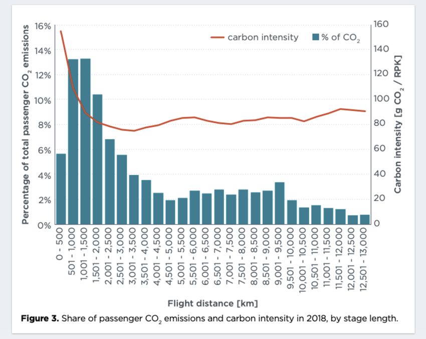
footprint begins to be linear as the distance value increases [ICCT, 2019].
In Annex A.5 you can see the graph of [ICCT, 2019] that determines the amount
of CO2 proportional to a passenger per km (gCO2 / Revenue Passenger
Kilometers (RPK)) according to the distance of the trip. Using the information in11
this graph, a model has been developed capable of calculating the total
emissions of a passenger according to the distance of the trip (kgCO2 / km).
The equations resulting from this model are the following:
fair = 99.079 exp(0.1123 dair /1000); {100 < dair < 1500}
(1.8)
fair = 42.5 dair /1000 + 127.5; {dair > 1500}
(1.9)
Where fair is footprint calculated in Kg of CO2 and dair is distance in Km.
1.3. Train
The third and last means of transport used for this project is the train. The steps
used to obtain the cost, time and footprint data of rail travel are explained
below.
1.3.1. Distance
As seen in section 1.1.1, calculating the distance by train will be done using the
Google Directions API. The API allows searching for the route for rail transport
including the number of transports systems necessary to get from the origin to
the final destination. Therefore, the train distance that will be used in the
software in this case will be the sum of the distances of all the trains necessary
for this route. In this case the distance will be necessary to approximate the
price and the footprint.
1.3.2. Time
From the same Google Directions API’s request in section 1.3.1, the travel time
is obtained for each of the journeys made on the route. Carrying out different
searches, it is appreciated that the train journey between two points usually
requires a greater number of stopovers if the journey is not between two large
cities or, in the case of Spain, if the Alta Velocidad Española (AVE) high-speed
network does not arrive. This reason makes the dependence of time on
distance more difficult to achieve through a linear regression since the origin
and destination locations play an important role. For this reason, for the
software in section 3, the relative time values of each of the trains on the
journey, the number of stopovers and the total travel time are obtained directly
from the API.
A door-to-door route optimizer that includes sustainability criteria             12

           1.3.3.                   Price

Getting the price of train travel has a certain degree of complexity. As in section
1.2.3, train prices are adapted to the market and vary depending on the
software and the companies experts in charge of adjusting the price. In order to
estimate the value of prices trying to follow a pattern, a study has been carried
out along the same routes as in section 1.1.3. Through the official website of
National Network of Spanish Railways or Red Nacional de Ferrocarriles
Españoles (RENFE) the price for different routes has been analyzed by
comparing the price of the train ticket every day between one month and two
months in advance [RENFE]. The station of origin of this study has always been
Barcelona-Sants, the closest station to Castelldefels from which the vast
majority of medium and long-distance trains depart. As already happened in
section 1.1.3 future work wants to improve the accuracy of the software in price
searches for all types of stations, for example through a payment API that works
the same as the SkyScanner API, that allows us to know tickets price for free at
the time of the search. But for the experiments of this project it has been
deepened in knowing well the prices according to the day and the destination
from Barcelona. After this procedure, the price has been determined by a linear
regression, determined by the distance with a coefficient of determination of
0.94, see Equation (1.10).
This study also consists of interesting results such as the behavior of the price
with respect to the weeks in advance with which the search is carried out or the
variation that exists between one day of the week and another. All the results of
this study are attached in Annex A.6.

                                ctrain = 0.0623 dtrain + 7.1893             (1.10)

Where ctrain is cost calculated in € and dtrain is distance in Km.

           1.3.4.                   Footprint

The footprint calculation has been produced using the resources of
EcoPassenger, a web tool that behaves like a calculator to compare energy
consumption and CO2 emissions from different ways of transport. This software
is developed between the UIC, the Foundation for Sustainable Development,
German institute for energy and environmental research (IFEU) and HaCon
(software). These calculations are fed by the UIC Environment Strategy
Reporting System (ESRS) methodology [ESRS, 2016]. This calculator allows to
know, among other data, the carbon dioxide emissions for a rail route between
two stations. This resource has been used to take various samples and note the
relationship between distance and footprint. Doing the linear regression
between all the samples, equation (1.11) is obtained to approximate the
footprint with the distance of the trip.
13
ftrain = 0.0123 dtrain + 0.8136 (1.11)
Where ftrain is footprint calculated in Kg of CO2 and dtrain is distance in Km.
1.4. Energy resources
In the previous sections, the procedure used to calculate the footprint on the
different routes has been explained for each of the three means of transport,
taking into account the distance of the journey. This footprint is calculated from
the carbon dioxide emissions emitted only during the route. In order to more
accurately compare the environmental impact, the "Well to the wheels" process
of the energy sources used for these transportation systems, mainly gasoline,
diesel, kerosene and electricity, should be considered.
This chain begins with the extraction and processing of the primary energy
used, for example crude oil, gas... It continues with the transport in pipes, ships,
trucks or trains to the conversion plants and refineries. Finally, there is transport
to gas stations or warehouses in the case of fuel or transformation in the case
of electricity. From here, the energy is ready to be used in the corresponding
means of transport.
All these steps involve an energy expenditure. The efficiency of this process
depends on the efficiency of all the individual steps, the energy sources used
and the transport distances in each country. ESRS collects the energy
production data of each country used by EcoPassenger to compare energy
consumption, CO2 emissions and other environmental impacts between
different means of transport.
Thanks to EcoPassenger resources, a study has been carried out to compare
the energy resources used by each means of transport according to distance.
The searches used for this study were the same as those in section 1.3.4. in
which the footprint of the train with respect to the distance was determined
based on CO2 emissions. The results have been those of Fig 1.6.A door-to-door route optimizer that includes sustainability criteria 14
Car Airplane Train
Energy resources / Primary energy: Liter 120
105
90
of Gasoline equivalent
75
60
45
30
15
0
250 405 560 715 870 1025 1180 1335 1490 1645 1800
Distance (Km)
Fig. 1.6 Energy resources needed against distance for car, airplane and train
Analyzing the graph in Fig 1.6 we can see how, despite being the most polluting
means of transport, the amount of energy resources consumed to increase the
distance of the trip through the plane increases more slowly than that of the car
and the train. It is important to note that the calculations for the car are made
considering 1.5 passengers which is the European average utilization [Ifeu,
2010]. As already mentioned earlier in this project, a large part of the resources
used by the aircraft are destined for take-off and landing operations [ICCT,
2019], so the increase of these resources with distance is not affected in the
same way as its two other competitors.
1.5. Comfort
Another reason why a person makes the decision to opt for one means of
transport over another is the feeling that these produce when experiencing a
trip in them. Seat size, space, possibility of making a stop, sharing the seat next
to you with a known or unknown person, fears, phobias... There are many
subjective criteria that can affect the selection decision. All these reasons are
personal decisions and in this project they have wanted to collect under the
word comfort.
In order to work with comfort as one of the other three criteria that have been
seen so far (cost, time and footprint), an attempt has been made to find a
pattern that relates the comfort that a group of people perceives from each
transportation system according to the distance of the trip.
To this end, a survey of 127 people was carried out between January 15 and
17, 2021. The population in this survey was known people, mostly students and15
residents of the Catalunya region. The survey questions (visible in Annex A.7),
have been focused precisely on people residing in the region of Catalonia so
that the distance reference was the same for all. In this survey they have been
made to choose between the 3 types of transportation system to make different
trips to other cities. These cities coincide with those of the experiments in
section 4.
Car Airplane Train
8%
45 %
Valencia 49 % Madrid
55 % 37 %
6%
4% 3% 3%
18 %
Sevilla Paris
79 %
95 %
Fig. 1.7 Answers to the question: "What means of transport do you consider
most comfortable to go to the following destinations?"
For these 4 destinations the results have been mixed. For the shortest distance,
Valencia, the option chosen by practically half of the respondents was the car,
while the plane received only 6% of the votes. As destinations move away from
Catalonia, the trends for these two modes of transport are reversed. The plane
begins to feel more comfortable for a trip to Madrid, and it is the favorite option
for Seville. To travel to Paris the votes of the plane go up to 95%. On the other
hand, the car is no longer perceived as comfortable for distant routes, receiving
very few votes. The train, however, has been perceived as the best option forA door-to-door route optimizer that includes sustainability criteria 16 the trip to Madrid, receiving more than half of the votes for this medium-distance trip. The results of these four questions will be used to designate the value of comfort in the experiments in section 4. The routes chosen for these experiments include the cities mentioned in the survey, thus the method to assign a numerical value to comfort within the problem is to assign to each transportation system the percentage of votes they have received on each of the routes. Given the tendency of the three means of transport to be perceived as comfortable according to the distance of the trip, for the remaining routes of the experiment that are not those mentioned in this survey, an approximation has been made based on the trends of the three means of transport. In Annex A.8 you can see these approximations graphically. In any case, in order to find a more precise relationship between comfort and distance, it would be necessary to know the perception of users for more routes and for a larger population of respondents. All the methodologies to obtain data on the different means of transport seen in this section will be implemented in the optimization software. Section 3 explains how and when the necessary searches and calculations are carried out to obtain the input data of the problem and subsequently determine the best transport alternative for a route. The intermediate step between the input data and the output results will be seen in the next section, where the mathematics used to solve a problem is explained in which the objective is to determine the best alternative taking into account more than one criterion.
17

2.                MULTI-CRITERIA DECISION MAKING

Multi-Criteria Decision Making (MCDM) is a branch of a general class of
Operations Research models which deal with the process of making decisions
in the presence of multiple objectives [Pohekar and Ramachandran, 2004]. This
methodology allows finding the best feasible solution based on the established
qualitative criteria. This project requires a MCDM problem to find the best
transport alternative based on different criteria such as cost, time, footprint and
comfort. The MCDM methods can be divided into two: multi-attribute decision-
making (MADM) and multi-objective decision-making (MODM) methods [Hwang
and Yoon, 1981]. The difference between both methodologies is that in multi-
attribute problems, the alternatives are predetermined and the best solution
(best alternative) is achieved by comparing the alternatives with respect to their
attributes. For MODM the alternatives are not predetermined, a group of
objective functions is optimized under a series of limitations.
Within the MADM, one can distinguish between five types of methodologies
[Hajkowicz and Collins, 2007] [De Brito and Evers, 2016]:

     •   Scoring methods: simple methods based on the evaluation of
         alternatives using basic arithmetic. For example: SAW and CORPAS
     •   Pairwise comparision methods: useful methods to obtain the weights of
         the different criteria and evaluate subjective criteria by comparing the
         alternatives with each other. A well-known example is the Analytic
         Hierarchy Process (AHP) method
     •   Outranking methods: In this type of method, each solution shows a
         degree of dominance over the others in some criterion. Examples are the
         PROMETHEE and ELECTRE methods.
     •   Utility / value methods: This methodology implements degrees of
         satisfaction for each attribute of each alternative. Examples of these
         methods: MAUT and MAVT
     •   Distance-based methods: These methods calculate the distance
         between each alternative and a specific point. This point can be one that
         satisfies a number of conditions or a sweet spot between different
         attributes. An example of the latter case is the Higher Criteria
         Optimization And Compromise Solution or “Vlse Kriterijumska
         Optimizacija I Kompromisno Resenje” (VIKOR) method

For this project, the MCDM method used is the VIKOR method. The VIKOR
method orders the different alternatives of the problem (car, airplane and train)
by “closeness” to the ideal solution [Pohekar and Ramachandran, 2004] based
on the criteria established for each of them (price, time, footprint and comfort).
The objective to find a solution considered as optimal, will be to try to achieve
the lowest price, the shortest travel time and the smallest possible ecological
footprint, while the comfort criterion of each transportation system for the
distance of the trip is the greatest possible. A trade-off between all the criteria
will order the different transport alternatives from the optimal solution or best
solution, to the worst alternative.
A door-to-door route optimizer that includes sustainability criteria 18
2.1. VIKOR method
This section explains the steps of the VIKOR method to determine the “closest
to ideal” solution [San Cristobal, 2011] between the different means of transport.
This process begins by defining the objectives and criteria of the problem. For
this, it will be necessary to use the methodologies of section 1 to obtain
information on the different values that receive the criteria of cost, time, footprint
and comfort. With these values, a matrix is created from which the three
characteristic steps of the VIKOR method will be carried out. These steps will
allow obtaining a numerical value, called Q, which will allow us to compare the
alternatives from best to worst.
Next, Table 2.1 shows the matrix that will be used in this section to explain the
VIKOR method through an example. The alternatives are the rows of the matrix
and the criteria to take into account are the columns. The values in the matrix
are random data used only for the demonstration of this example of the VIKOR
method.
Table 2.1 Matrix of alternatives and criteria
Cost (€) Time (min) Footprint (Kg Comfort (%)
CO2)
Car 50 400 80 30
Airplane 90 90 150 30
Train 70 200 20 40
Once the problem matrix is defined, the three steps of the VIKOR method
begin. The first step will be to determine the f i* and f i− values that represent the
best and worst values of each criterion. This value will depend on each criterion,
if you want to maximize or minimize the value of each of them. In this case, it is
wanted to minimize cost, price and footprint, but instead comfort is a criterion to
be maximized since the objective is to obtain the highest percentage possible.
Table 2.2 shows these values named “best" (f i*) and “worst" (f i−) according to
the desire to maximize or minimize the result of the criterion.19
Table 2.2 Step 1: Best and worst values f i* and f i−
Cost (€) Time (min) Footprint (Kg Comfort (%)
CO2)
f i* 50 90 20 40
f i− 90 400 150 30
The second step is to calculate the Sj and Rj values. These values are unique
for each of the alternatives and correspond to the mathematical formulas (2.1)
and (2.2) respectively. In order to calculate these values, the fixed values of
Table 2.2 and the weight that each alternative receives are necessary. The
weight corresponds to the percentage of relative importance that each of the
criteria receives. The objective is to capture the preferences of passengers on
the different criteria and convert this subjective information into percentage
weights. The methodology for assigning weights used to carry out the
experiments in section 4 will be detailed in section 2.2 For the explanation
example of this section, the weights (wi) used are also random and correspond
to the following: 30% cost, 35% time , 20% footprint, and 15% comfort. This is
more important for time and cost values and less important for footprint and
comfort.
n
wi( f i* − fij )/( f i* − f j−)
∑
Sj = (2.1)
i=1
Rj = m a xi[wi( f i* − fij )/( fi * −fi)] (2.2)
Using formulas (2.1) and (2.2) for the example, the Sj and Rj values of Table 2.3
corresponding to each of the alternatives are obtained.
Table 2.3 Step 2: Sj and Rj for each alternative
Sj Rj
Car 0,592 0,35
Airplane 0,65 0,3
Train 0,274 0,15A door-to-door route optimizer that includes sustainability criteria 20
The third step will be to determine the Qj value. The Qj value is what allows us
to rank the “closest to ideal” solutions [Pohekar and Ramachandran, 2004]. It
will be done from equation (2.3) and it will be necessary to use the values of S*,
S − and R*,R − that represent the maximum and minimum value of Sj and Rj as
it happened in the first step. ν is used as a group maximum utility weight [1]. It
takes values between 0 and 1 but normally 0.5 is used. In this example we will
use 0.5
Qj = ν(Sj − S*)/(S − − S*) + (1 − ν)(Rj − R*)/(R − − R*) (2.3)
The goal is for the results of Qj to be 0 or as close to 0. This will determine the
best solution. The ranking from best to worst alternative will be determined by
Qj values from lowest to highest. Table 2.4 shows the results of Qj through
formula (2.3) for this example of the VIKOR method.
Table 2.4 Step 3: Qj for each alternative
Q
Car 0,923
Airplane 0,875
Train 0,0
In the case of this example, the VIKOR method has determined that for the
values in Table 2.1 and with weights of: 30% cost, 35% time, 20% footprint and
15% comfort, the best solution is the train, the second best option would be the
airplane and finally the car.
The last step of the VIKOR method involves validation of the compromise
solution through two criteria:
• "Acceptable advantage": The condition Q (A(2) - Q (A(1))> = DQ is met;
where A(1) is the alternative with the lowest value of Q, A(2) the second
best alternative and DQ = 1 / (J-1).
• "Acceptable Stability in decision making": Alternative A(1) apart from
having the best value of Q must also have the minimum value of S and /
or R.You can also read