Integrating climate, health, resilience, and bill savings into the cost-optimal deployment of solar plus storage on public buildings

Integrating climate, health, resilience, and bill savings into the cost-optimal
 deployment of solar plus storage on public buildings

 by

 Amanda Farthing

 A thesis submitted
 in partial fulfillment of the requirements
 for the degree of
 Master of Science
 (Environment and Sustainability)
 in the University of Michigan
 April 2021

Thesis Committee:
 Professor Michael Craig, Co-Chair
 Professor Tony Reames, Co-Chair

This page is intentionally left blank.

Abstract
Climate change, public health, and resilience to power outages are of critical concern to local
governments and are increasingly motivating investments in on-site solar and storage.
However, designing a solar plus storage system to co-optimize for climate, health, resilience,
and energy bill benefits requires complex trade-offs that are not captured in current analyses.
To fill this gap, we integrate climate and health benefits into the REopt Lite optimization model
using forward-looking, location-specific marginal emissions factors and health costs. Using
this novel framework, we quantify the impact of including energy bill, climate, health, and/or
resilience benefits on the cost-optimal sizing, battery dispatch, and economic returns of solar
plus storage on three public building types across fourteen U.S. cities. We find that monetizing
and optimizing for climate and health benefits, as compared to only energy bill savings and
resilience, increases the net present value of the modeled solar plus storage systems by $0.2
million to $5 million. Due to changes in the cost-optimal battery dispatch, our expanded
optimization results in additional climate and health benefits of $0.50 per dollar invested, as
compared to optimizing for only energy bill savings and resilience. Our results illustrate
significant differences across geographies and building types, highlighting the need for site-
specific analyses of the costs and benefits of solar plus storage.

 i

Acknowledgements
This material is based upon work supported by the National Science Foundation Graduate
Research Fellowship under Grant No. DGE 1841052. This research was informed by valuable
insights from the City of Ann Arbor Office of Sustainability & Innovations, the Washington
D.C. Department of Energy & Environment, and the National Renewable Energy Laboratory
Modeling and Analysis Group. This work would not have been possible without the guidance,
expertise, and support of my advisors, Dr. Michael Craig and Dr. Tony Reames.

I would also like to thank my parents and sister—Colin, Lisa, and Heather—for their
unwavering love and support throughout the peaks and valleys of the last two years.

 ii

Table of Contents
 Abstract .............................................................................................................................................. i
 Acknowledgements........................................................................................................................... ii
 List of Acronyms and Abbreviations ............................................................................................ iv
 1. Introduction .................................................................................................................................. 1
 2. Methods ......................................................................................................................................... 3
 2.1 REopt Lite Modeling Framework ............................................................................................................ 3
 2.2 Valuing Benefits of Reduced Emissions.................................................................................................. 4
 2.2.1 Marginal emissions rates....................................................................................................................... 4
 2.2.2 Climate benefits .................................................................................................................................... 6
 2.2.3 Health benefits ...................................................................................................................................... 7
 2.3 Valuing Benefits of Increased Resiliency ................................................................................................ 8
 2.4 Model Application across United States .................................................................................................. 9
 2.5 Sensitivity Analysis ............................................................................................................................... 14
 3. Results ......................................................................................................................................... 15
 3.1 Cost-Optimal System Sizing .................................................................................................................. 15
 3.2 System Economics ................................................................................................................................. 16
 3.3 Optimal Battery Dispatch ...................................................................................................................... 19
 4. Discussion .................................................................................................................................... 21
 References ....................................................................................................................................... 23
 Appendix A: Discussion of marginal emissions rates scaling approach ................................... 31
 Appendix B: Supplementary tables and figures.......................................................................... 32
 Appendix C: Sensitivity analysis .................................................................................................. 39

 iii

List of Acronyms and Abbreviations

BAU business as usual
CAIDI Customer Average Interruption Duration Index
CapEx capital expenditures
CRB Commercial Reference Building
DER distributed energy resource
DSM demand side management
EPA U.S. Environmental Protection Agency
ITC investment tax credit
k thousand
kW kilowatt
kWh kilowatt hour
LCC life cycle cost
LMP locational marginal price
M million
MACRS modified accelerated cost recovery system
MW megawatt
MWh megawatt hour
NEEDS National Electric Energy Data System
NEM net energy metering
NERC North American Electric Reliability Council
NPV net present value
NREL National Renewable Energy Laboratory
O&M operations and maintenance
PV photovoltaics
REC renewable energy credit
ReEDS Regional Energy Deployment System
REopt Lite NREL’s Renewable Energy Optimization Lite model
ROI return on investment
SOC state of charge
solar plus storage solar photovoltaic and/or battery storage systems
SRMER short-run marginal emissions rate
t metric ton
TOU time of use
VDER value of distributed energy resources
VoLL value of lost load
VOS value of solar

 iv

1. Introduction
In the United States, the electricity sector accounts for 25% of greenhouse gas emissions1 and
11% of air pollution-induced premature mortalities.2 As extreme weather events increase,3 the
U.S. power system is also seeing more frequent “major disturbances and unusual
occurrences”—increasing tenfold from 2000 to 20204 and resulting in economic losses and
loss of life.5,6 Moreover, the burdens of climate change, air pollution, and power outages result
in stark inequities—having been shown to disproportionately impact people of color and less
affluent communities.7–11

With the ability to offset emissions from grid-purchased electricity and to provide power
during blackouts, on-site solar photovoltaics and battery storage (solar plus storage) are well-
poised to simultaneously reduce climate, health, and outage damages along with the system
owner’s energy bill costs. Grid-connected distributed solar installations in the U.S. have grown
over the past two decades, from just under 800 annual installations in 2000 to over 374,000 in
2019 (Figure 1).12 Meanwhile, the percentage of these systems that integrate storage has also
increased to a respective 1.4% and 5% for small and large non-residential systems in 2019
(Figure 1) and is expected to continue to grow.13,14

 400
 U.S. Grid-Connected, Percent of PV Systems in
 Distributed PV 14% Full Sample with Storage
 Small Non-Residential
 12%
Number of Systems

 Large Non-Residential
 10%
 (1,000s)

 8%

 6%

 4%

 2%

 0 0%
 2000 Installation Year 2019 2016 2017 2018 2019

Figure 1. (left) Number of annual installations of grid-connected distributed PV in the U.S. and
(right) storage attachment as percentage of installed distributed PV systems (Source: LBNL Tracking
the Sun 2020).12,14

Given the increasing adoption of solar plus storage, many analyses quantify various costs and
benefits of these technologies in diverse siting and operational contexts. A comprehensive
understanding of the costs and benefits of solar plus storage can inform policy instruments
(e.g., value of distributed energy resources (VDER) tariffs),15–17 insurance valuations,18 equity
considerations,19–22 investment decisions,23–26 and operational strategies.27–29 However,
capturing the collective impact of climate, health, resilience, and energy cost savings within
the cost-optimal deployment of solar plus storage remains a challenge that has yet to be
addressed.

When paired with microgrid technologies (e.g., appropriate inverters, controls, and electrical
infrastructure),30 solar plus storage can increase resilience, keeping critical loads powered
when the primary grid is down. Particularly in the context of critical services and resilience

 1

hubs, powering loads through an outage can reduce economic losses and mitigate suffering or
loss of life. Considering resilience within solar plus storage system design can result in larger
cost-optimal systems and increased resilience.23,24,31 The value of resilience is typically defined
as the economic value of avoided outages, calculated as the quantity of load powered through
an outage multiplied by a value of lost load (VoLL).18,24,32–35 Estimates of VoLL in the
literature vary widely due to differences in methodologies (e.g., macroeconomic vs.
willingness-to-pay studies), the end user-group studied, and the assumed outage duration.33
Many previous studies have addressed and optimized for microgrid resilience.23,24,36–42 Laws
et al. (2021) provides the first model to co-optimize microgrids for annual grid-connected and
resilience benefits under uncertain outages, while accounting for additional islanding costs and
arbitrary utility tariff structures.43 In this study, we build upon the work of Laws et al. (2021),
which is implemented in the National Renewable Energy Laboratory’s (NREL’s) open source
REopt Lite model,44 by further integrating climate and health impacts.

Analyses of climate and health benefits of distributed energy resources (DERs) typically focus
on solar energy (without the time-shifting ability of storage) and assume pre-determined
system sizes.19,45–47 When assessing the emissions impacts of an incremental change in
electricity consumption, it is recommended to assume an associated change in production from
the marginal generator, rather than considering the average emissions intensity of the grid.48,49
Many studies assume that the marginal generator is always a natural gas plant,16,17,50,51 while
others assume that the marginal generator differs between off-peak and on-peak hours,52 varies
hourly based on dispatch modeling results,53 or utilize regressions of historical generation and
emissions levels to estimate marginal emissions factors.19,47 Studies that have addressed the
combined emissions impact of solar plus storage have done so in the context of isolated
microgrids,54–57 predefined schedules of demand response actions,58 while optimizing battery
dispatch for alternative objectives (e.g., reducing grid reliance),27 or while considering general
life cycle assessment emissions factors for technology components.59,60 Avoided CO2
emissions are typically valued using the social cost of carbon from the U.S. Interagency
Working Group.19,61–63 Avoided criteria air pollutants are typically valued as the compliance
cost for emissions reductions from power plants or the estimated cost of medical expenses or
mortality risk from emissions, although these damages are less frequently explicitly recognized
in value of distributed solar literature and policies.15,16,64

We extend the literature by incorporating climate and health impacts, along with resilience,
into the cost-optimal sizing of grid-connected solar plus storage. In contrast to previous work,
we use location-specific and forward-looking marginal emissions factors and location- and
season-specific marginal health costs. Valuation of climate and health impacts is particularly
relevant for local governments, who own numerous properties, are responsible for wellbeing
of their constituency, and are increasingly making climate commitments.65 Resilience is also
particularly salient for local governments, given that they must maintain power to critical
infrastructure during blackouts, often provide the first line of response during disasters, and
are well-poised to create resilience hubs to serve vulnerable community members.66,67

Using our model, we quantify the impact of including climate, health, and/or resilience costs
and benefits on the optimal system sizes, economic returns, and battery dispatch of solar plus
storage projects for three public building types across 14 U.S. cities. Our analysis demonstrates

 2

how local governments’ cost-optimal deployment of solar plus storage would change when
considering the costs of emissions damages and power outages in conjunction with investment
costs and energy bill impacts.

2. Methods

2.1 REopt Lite Modeling Framework

To quantify climate and health impacts of solar plus storage, we incorporate forward-looking
marginal emissions costs of grid-purchased electricity into the National Renewable Energy
Laboratory’s (NREL’s) Renewable Energy Optimization (REopt) Lite model, an open-source
Julia package.44 To quantify the value of resilience, we utilize the method from Laws et al.
(2021).43

When applied to solar plus storage systems, the REopt Lite model seeks to minimize the life-
cycle cost (LCC) of electricity purchases by determining optimal technology sizes and the
hourly storage dispatch strategy. For the full formulation of REopt, see Cutler, et. al. (2017).68
Within the model, the utility costs, building load, and renewable generation in year one are
assumed to represent a typical year. REopt Lite thus solves a single-year optimization, ensuring
operational constraints are met in each hour, to determine year one cash flows. Cash flows for
subsequent years are adjusted based on user-supplied rates of change for future costs (e.g.,
utility and O&M costs) and are discounted to determine the LCC of an investment.

Prior to our work, REopt Lite’s solar plus storage life-cycle cost minimization included capital
costs (Ccap), operations and maintenance costs (CO&M), the net cost of utility-purchased
electricity (Celec), and resilience costs (Cmaxoutage and Cmg). We extend this optimization to
include climate (Cclimate) and health (Chealth) costs such that our objective becomes:

 = !"# + $&& + '('! + )"*$+,"-' + )- + !(.)",' + /'"(,/ (1)

The value of resilience is captured by Cmaxoutage, which represents the maximum outage cost
and Cmg, which represents the cost to enable the microgrid system to operate in isolation from
the grid.43 Cclimate and Chealth represent climate and health costs, respectively, associated with
grid-purchased electricity.

The net electricity cost (Celec) represents energy and demand charges minus compensation for
net exports to the grid. The calculation of energy bill savings given an arbitrary utility tariff is
described in the REopt Lite documentation.69 In this work, we incorporate traditional cost
considerations, as well as resilience, but focus mainly on the valuation of climate and health
benefits.

Figure 2 provides high-level model inputs, data sources, and relevant sections of this paper.

 3

Figure 2. Overview of model inputs and outputs, along with relevant sections of this paper related to
the valuation of climate, health, and resilience benefits.

The net present value (NPV) of a proposed investment is calculated as the difference between
the “business-as-usual” (BAU) life-cycle costs (LCCBAU)—in which a building has neither
solar nor storage—and the “investment case” life-cycle costs (LCCinv)—in which the model
determines the optimal system sizes (Eq. 2).

 = 012 − .34 (2)

If the given investment in solar and storage results lower lifetime costs than the BAU case,
then the NPV will be positive, and the investment is considered cost optimal. Analogously, we
define the net climate, health, and resilience benefits of solar plus storage as the difference
between these respective costs in the BAU and investment cases.

2.2 Valuing Benefits of Reduced Emissions

We quantify the climate and health benefits of solar plus storage based on reduced emissions
from grid-purchased electricity due to these technologies. We do not account for upstream or
end-of-life emissions associated with solar or storage. We estimate the hourly costs (or
damages) of CO2, SO2, and NOx as the product of each pollutant’s marginal emissions rate,
marginal damage cost, and net load. The hourly net load reflects net grid purchases, i.e., grid-
purchased electricity minus any exports to the grid from the battery and/or PV system.

2.2.1 Marginal emissions rates

We assume a change in grid-purchased electricity in a given hour due to on-site solar and
storage results in an associated increase or decrease in generation from the marginal energy
source. We obtain forward-looking hourly marginal energy source data at the balancing area
scale from NREL’s Cambium database.70 We utilize the marginal energy source (as opposed
to marginal generator) to account for time-shifted generation needs resulting from energy-
constrained marginal generators (e.g., batteries).71 Cambium datasets are based on projected
generator fleets from the Regional Energy Deployment System (ReEDS) model72 and hourly
fleet operations from the PLEXOS production cost model.73 Modeled grid data are available
for every other year between 2018 and 2050; we assume odd-numbered years have the same
generation profile as the previous even-numbered year. We use results from the Mid-Case
Scenario, which assumes default or median model inputs regarding the future generation mix
and includes existing policies as of June 2020.74

 4

From the hourly marginal energy source, we obtain marginal emissions rates for pollutants that
impact the climate (carbon dioxide (CO2)) and public health (sulfur dioxide (SO2) and nitrogen
oxides (NOx)), for each year of the analysis period (2021-2046).

For climate damages, we consider only emissions of CO2. While pollutants such as methane
(CH4) and nitrous oxide (N2O) also contribute to climate damages, the CO2-equivalent
emissions of non-CO2 pollutants are relatively small for grid-sourced power.69 We utilize
hourly short-run CO2 marginal emissions rates (SRMERs) from Cambium at the balancing
area scale. The hourly SRMER (t CO2/kWhenduse) is the end-use emissions rate of the marginal
energy source and is already adjusted for transmission, distribution, and efficiency losses in
delivery to the end user.

For health damages, we consider only the impacts of SO2 and NOx, which affect human health
through their secondary formation of PM2.5. Together, these species account for
approximately 82% of mortalities caused by power plant emissions (~75% from SO2 and 7%
from NOx).75 Direct emission of PM2.5 also contributes a significant amount (~14%) to PM2.5
exposure and associated mortalities from the electricity sector and should be considered in
future work.75 Future marginal emissions rates for criteria air pollutants are not available from
Cambium or other public datasets. Instead, we calculate historic plant-level emissions rates for
SO2 and NOx using the U.S. Environmental Protection Agency’s (EPA’s) National Electric
Energy Data System (NEEDS) v6 database of U.S. power plant characteristics.76 We calculate
each plant’s SO2 and NOx emissions rates [t/kWh] as the heat rate [Btu/kWh] multiplied by
the SO2 Permit Rate [lbs/mmBtu] and Mode 4 NOx Rate [lbs/mmBtu], respectively. We use
the Mode 4 NOx Rate, which assumes state-of-the-art combustion controls are in place, in
anticipation of these controls becoming more widely adopted. We subsequently calculate the
average SO2 and NOx emissions rates by plant type and NEEDS region. NEEDS regions
generally represent subdivisions of the 8 North American Electric Reliability Council (NERC)
regions. We map region- and plant type-specific SO2 and NOx emissions rates to the
corresponding hourly marginal energy source in the corresponding Cambium balancing area
using the mapping scheme in Table B1.

The resulting average hourly marginal emissions rates (merplant) for SO2 and NOx are
subsequently adjusted for transmission and distribution losses using the hourly marginal
distribution loss rate (Lyr,hr) as reported in the Cambium dataset.71 As a result, we obtain end-
use marginal emissions rates (merenduse) for SO2 and NOx for each hour (hr) of the year, for
each year (yr) of the analysis period (Eq. 3).

 '38+9' #("3, (3)
 mer56,/6 = mer56,/6 ∗ 31 + 56,/6 5

Since the REopt Lite model determines an optimal hourly battery dispatch strategy for a single
year, we cannot utilize hourly marginal emissions rates with profiles that vary year to year.
Instead, to account for both hourly variability and annual trends, we select the midpoint year
of the analysis to represent the profile (or shape) of the marginal emissions rates for CO2, SO2,
and NOx. We then scale the mid-point year hourly profiles based on the respective total
marginal emissions of CO2, SO2, and NOx in each year of the analysis.

 5

For a 25-year analysis beginning in year 2021, we thus have three sets of 25 marginal emissions
profiles (merhr,yr ) that reflect the CO2, SO2, and NOx hourly marginal emissions shape of 2033
(each hour is scaled from the corresponding hour in 2033), but maintain the total per kWh
damage from marginal emissions over each analysis year. Figure 3 shows an example of the
resulting hourly profiles over a 24-hour period for 2021-2046. Selecting the profile of the
midpoint year accounts for the fact that more emissions-intensive generators are on the margin
less often as the years progress from 2021 to 2046 and thus avoids over- or under-sizing the
system. For further explanation and justification of this approach, see Appendix A.

 CO2 SO2 NOx
 0.001
 1.4

 1.2 0.0008
 0.01
 1
t/MWh

 t/MWh

 t/MWh
 0.0006
 0.8
 0.005
 0.0004
 0.6

 0.4 0.0002
 0
 5 10 15 20 5 10 15 20 5 10 15 20

 Hour of day Hour of day Hour of day
Figure 3. Example CO2 (left), SO2 (center), and NOx (right) hourly marginal emissions rates, scaled to
reflect the shapes of the 2033 (mid-point year) hourly profiles. Example shown is for the city of
Chicago for one day for the years 2021-2046.

2.2.2 Climate benefits

To monetize the social damages caused by CO2 emissions, we use the social cost of carbon
dioxide (SC-CO2) from the U.S. government’s Interagency Working Group.63 For our baseline
scenario, we utilize $52 per metric ton of CO2 (in $2020 assuming a three percent discount
rate). Consistent with the literature, we assume marginal damage costs in each year of the
system’s lifetime can be approximated by this 2020 marginal damage cost (prior to
discounting).19,59,61

 !(.)",'
We calculate the total climate damage cost ( 56 ) in each year (yr) of the analysis period
(A) as:
 !(.)",' = - ∗ 9 3 ∗ 5 ∀ ∈ (4)
 56 ; /6 /6,56

The total climate-related cost (Cclimate) is calculated as the NPV of the annual climate costs,
using the electricity off-taker’s discount rate (d) (Eq. 5). This total cost is incorporated into the
model objective in scenarios in which climate costs are considered.
 !(.)",' (5)
 !(.)",'
 56
 = = 9
 (1 + ) 56
 56∈1

The climate benefit ( !(.)",' ) of a given system is the difference between the climate costs
 !(.)",' !(.)",'
in the BAU ( 012 ) and investment cases ( .34 ) (Eq. 6). The climate benefit can be
negative.

 !(.)",' !(.)",'
 !(.)",' = 012 − .34 (6)

2.2.3 Health benefits

The marginal health damage of air pollutants is highly dependent on the local population and
atmospheric conditions.77 These marginal damages are also highly seasonally-dependent, with
a U.S. average of 80% of power plant mortality damages attributable to emissions from April
to September.75 To estimate location- and season-specific marginal health damages for
emissions of SO2 and NOx, we use the Estimating Air pollution Social Impact Using
Regression (EASIUR) model.78 EASIUR utilizes reduced-form air quality modeling to
estimate the increase in public health burden caused by a marginal increase (one additional
metric ton) of PM2.5 precursor emissions (including SO2 and NOx) in a given location. Public
health burden is calculated as an increase in mortality (premature deaths) in downwind
populations caused by inorganic PM2.5 exposure, using a $8.6 M ($2010) value of statistical
life (VSL) and a concentration-response relation from the American Cancer Society.77 The
resulting marginal damage costs are available at a resolution of 36 km x 36 km, for each of the
four seasons, for three emissions elevations (ground-level, 105 m, and 300 m). We assume
emissions occur at the building location, given that the exact location of the marginal energy
source is not available. We assume the income and population year is 2021 and adjust the
results to $2020. We use seasonal estimates for 105 m elevation, given that most power plants’
stack heights are at or below this height.79 Similar to our approach to the SC-CO2, we assume
that damage estimates in each year can be approximated by 2021 damage estimates (prior to
discounting). Previous studies have shown annual damages obtained from EASIUR to be
comparable to, yet slightly lower than, damage estimates obtained using other integrated
assessment models, e.g., AP219 and AP3 and inMAP.61
 /'"(,/
We calculate the annual health damage cost ( 56 ) for each year (yr) of the analysis period
(A = {0, 1, 2,...,n}) as:

 #$%&'#
 !" = # # $mec(
 )*! /0
 ∗ netload#" ∗ +,,.,
 !
 + c(
 1*" 1*
 ∗ netload#" ∗ mer#",!"
 "
 5 ∀yr ∈ A (7)
 (∈) #"∈)3"

where s indexes the season in S={winter, spring, summer, fall} and the seasonal marginal
emissions costs for SO2 and NOx (mecSO2 and mecNOx) are in units of $2020/t of pollutant. The

 7

marginal costs are each multiplied by the hourly net load (netload [kWh]) and hourly end-use
marginal emissions rates (mecSO2 and mecNOx [t/kWh]), for each hour (hr) in the set of hours
corresponding to each season (SHr). The annual health cost is the sum of damages from SO2
and NOx over each hour of the year.

The public health cost (Chealth) over the lifetime of the system is calculated as the NPV of the
 /'"(,/
annual health costs ( 56 ), using the electricity off-taker’s discount rate (d) (Eq. 8). This
total cost is incorporated into the model objective in scenarios in which health costs are
considered.
 /'"(,/ (8)
 /'"(,/
 56
 = = 9
 (1 + )56
 56∈1

The health benefit ( /'"(,/ ) of a given system is the difference between the health costs in
 /'"(,/ /'"(,/
the BAU ( 012 ) and investment cases ( .34 ) (Eq. 9). The health benefit can be
negative.

 /'"(,/ /'"(,/
 /'"(,/ = 012 − .34 (9)

2.3 Valuing Benefits of Increased Resiliency

The methods used to value resilience within the REopt Lite Julia Package and the associated
model constraints are described in previous work.43 Below, we summarize key components of
the valuation approach with slight modifications considering the unique assumptions of this
research.

The outage cost is the maximum expected outage cost (Cmaxoutage) over set T of possible outage
start times (t0). We assume the outage occurs annually and adjust the annual cost with a present
worth factor (pwf):

 A+,"-'
 )"*A+,"-' = max J ,4 K ∗ , ∀ B ∈ (10)
 ,4

In our baseline scenario, we consider an outage of 15 hours, the average duration of major
outages in 2020,4 occurring with 100% probability. Ideally, we would model the outage at each
hour of the year for every scenario; however, this approach proved computationally intractable.
To reduce the computational intensity of the models while still capturing the uncertain nature
of major outages, we determine the set of outage start times (T) for each building that results
in the 95th percentile of total unserved load in absence of a microgrid. That is, we simulate a
15-hour outage in each hour of the year (assuming no microgrid exists), determine the 438
hours that represent the 5% worst times to experience an outage, and use this set T in all
optimization scenarios for that building. Appendix B includes histograms showing the outage
start hours in set T by month and hour of the day.

 8

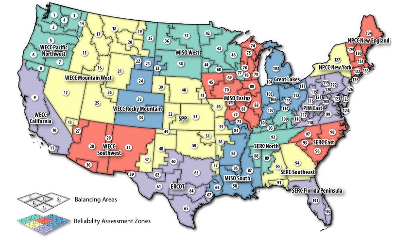
The cost of each simulated outage is the value of lost load (VoLL) [$/kWh] multiplied by the
total unserved load (UL) over all hours (hr) of the outage (where the outage starts at time t0
and lasts until time t0+d):
 
 A+,"-'
 = ∗ 9 (11)
 ,4 /6
 /6∈$+,"-'

Estimates of the VoLL for public buildings are limited. Given the far-reaching impacts of an
outage to public facilities—which may provide core health or safety services or be a resilience
hub for residents66,80—we utilize economy-wide estimates of the VoLL. Several review papers
show that economy-wide estimates for mid- to long-duration outages fall within $4-
$40/kWh81–84 (in varying dollar years) while others have estimated the cost of a 16-hour power
outage in the U.S. to range from $70-$140/kWh (in $2020) when accounting for indirect
impacts.81

In this research, we draw upon these wide-ranging estimates and assume that the economy-
wide impacts of a mid-duration (15-hour) outage has a minimum cost of $4/kWh and a
maximum cost of $140/kWh. We subsequently estimate outage costs for different public
facility types based on whether they provide critical or emergency services and whether they
will serve as a resilience hub for community members during an outage (Table 1). Critical or
emergency facilities are assumed to incur costs at the high end of our defined range. We
estimate the cost of an outage to a resilience hub to be the midpoint value and the cost to a non-
critical and non-resilience hub facility to be at the low end of the range. VoLL is assumed to
be constant throughout the year. This approach to differentiating the VoLL is unique and is
constrained by limited data for public facilities; future research in this area will be valuable.

Table 1. Estimated VoLL for different public facility types for a 15-hour outage.

 Facility type VoLL ($2020/kWh)
 Critical or Emergency Service $140
 Resilience Hub $72
 Non-critical, Non-resilience Hub $4

The resilience benefit ( 6'9.(.'3!' ) is calculated as avoided outage costs minus the microgrid
upgrade cost.
 )"*$+,"-' )"*$+,"-' )- (12)
 6'9.(.'3!' = ( 012 − .34 ) − .34

2.4 Model Application across United States

We apply our model to three public building types (hospital, secondary school, and warehouse)
in 14 U.S. cities (Albuquerque, Atlanta, Baltimore, Boulder, Chicago, Duluth, Helena,
Houston, Los Angeles, Miami, Minneapolis, Phoenix, San Francisco, and Seattle). These
building types serve differing roles during a power outage: a hospital provides critical services,
a secondary school can serve as a community resilience hub, and a warehouse may serve no
special role. For each building, we determine the cost-optimal solar plus storage system size

 9

and economic outcomes when considering bill savings, resilience, climate, and/or health
impacts (Table 2). Our 14 locations span unique climate zones and balancing areas (Figure
4).71,85,86 We assume each building has already been deemed suitable for solar given, e.g., roof
vintage and loading capacity.

 Seattle, WA

 Duluth, MN
 Helena, MT

 Minneapolis, MN

 San Francisco, CA Chicago, IL

 Baltimore, MD
 Boulder, CO

 Albuquerque, NM

 Los Angeles, CA Atlanta, GA
 Phoenix, AZ

 Houston, TX

 Miami, FL

Figure 4. Locations for buildings modeled in this study along with balancing areas and reliability
assessment zones used to develop Cambium datasets (Source: Cambium Documentation 202071).
(MISO: Midcontinent Independent System Operator; NPCC: Northeast Power Coordinating Council;
SERC: SERC Reliability Corporation; SPP: Southwest Power Pool; WECC: Western Electricity
Coordinating Council)

Table 2. Optimization scenarios, associated acronyms, and LCC calculations used in this study.

 Monetized
Acronym value streams Objective value (minimization)
 B Bill savings = !"# + $&& + '('!
 Bill savings,
 BR = !"# + $&& + '('! + )"*$+,"-' + )-
 resilience
 Bill savings,
 BRCH resilience, = !"# + $&& + '('! + )"*$+,"-' + )- + !(.)",' + /'"(,/
 climate, health

We hold several inputs constant across locations, including project finance assumptions (Table
3); technical and cost assumptions for PV and battery storage (Table 4); anticipated outage
characteristics (Table 5); available roof space for solar by building type (Table 6); critical load
percentage by building type (Table 6); VoLL by building type (Table 6); and the social cost of
carbon. Inputs we vary across locations are building loads (Table B2); marginal emissions
costs (Figure 5); marginal emissions rates of grid-purchased electricity; utility tariff
assumptions (Table B3); and net energy metering (NEM) rates.

Given the 25-year life a PV system, we run our analysis from 2021 to 2046. We assume the
projects are directly owned and entirely financed by the local governments, and thus we do not

 10

consider tax benefits (e.g., MACRS and ITC). Incorporating alternative financing models,
while outside the scope of this research, could make investments more financially attractive
for local governments.

In our baseline scenario, we assume an annual outage of 15 hours (the average duration of
major U.S. outages in 20204). We estimate the critical load for each facility based on whether
it provides critical services or could serve as a resilience hub during a power outage. The
building-specific VoLL is accordingly assigned using the values from Table 1.

Climate zone-specific building loads are generated from the U.S. DOE Commercial Reference
Building (CRB) models for post-1980 construction for each site.85 We estimate the total roof
area that is suitable for solar as the corresponding CRB total square footage (which is constant
across climate zones) divided by number of floors. We assume 50% of the roof is available to
host solar panels.

We use a SC-CO2 of $52/t ($2020) for all analyses. Figure 5 shows the marginal health costs
from EASIUR of SO2 and NOx by season and location. Marginal health costs are notably higher
in Baltimore, Chicago, Los Angeles, San Francisco, and Seattle than the average across all
cities, marked by the solid horizontal line. Average marginal CO2, SO2, and NOx emissions
rates from 2021-2046 for each location are shown in Figure 6. While these averages illustrate
the difference in emissions-intensity of grid electricity in the 14 locations, in our analysis we
utilize hourly marginal emissions rates as described in Section 2.2.

We model realistic utility rate structures by selecting an appropriate tariff for each building
from the International Utility Rate Database, based on the likely utility company given the
location and any applicable energy or demand limits87 (Table B3). Many of these rates include
time-of-use components. The REopt Lite Julia package simplifies multi-tiered rates by using
the first tier for energy rates and the last tier for demand rates.44 For the sake of comparison,
Table B3 includes the average energy and demand rates in the base case (without solar or
storage technologies). We assume net energy metering (NEM) is permitted for all buildings
and that net excess generation is compensated at the retail rate. All model instances were solved
using the IBM® CPLEX® Optimizer.

Table 3. Financial assumptions for all buildings. All financial values are nominal.

 Parameter Value
 Analysis period 2021-2046
 Discount rate 8.3%*
 O&M cost escalation rate 2.5%*
 Electricity cost escalation rate 2.3%*
 Tax rate 0%
 ITC Not applied
 MACRS Not applied
*These values are the REopt Lite default values, which draw largely from national averages. See documentation
 for sources and assumptions.69

 11

Table 4. Technical and cost assumptions for PV, battery storage, and microgrid systems for all
buildings. All financial values are nominal.

 PV Assumptions Value
 Technical
 Annual degradation 0.5%*
 Rooftop power density 10 watts / sf*
 Inverter efficiency 96%*
 System losses 14%*
 DC/AC ratio 1.2*
 PV tilt 10 degrees*
 Module type Standard*
 Azimuth 180 degrees*
 Hourly PV production Obtained from PVWatts using
 location and system characteristics
 Economic
 Installed cost $2.3/W**
 O&M cost $16/kW/year*
 Battery Assumptions Value
 Technical
 Inverter and storage replacement Year 10*
 Total AC-AC round trip efficiency 89.9%
 Internal efficiency 97.5%*
 Inverter efficiency 96%*
 Rectifier efficiency 96%*
 Minimum/initial state of charge 20% / 50%*
 Can grid charge battery? Yes
 Economic
 Installed cost $840/kW, $420/kWh*
 Replacement cost (year 10) $410/kW, $200/kWh*
 Microgrid Assumptions
 Economic
 Microgrid premium 30% of solar plus storage capital
 cost*
*These values are the REopt Lite default values, which draw largely from national averages. See documentation
 for sources and assumptions.69
 **U.S.-wide median cost for large non-residential PV systems in 2019.14

Table 5. Anticipated outage characteristics

 Parameter Value
 Outage length 15 hours
 Outage start times Hours in the 95th percentile of most
 unserved load in absence of microgrid
 Outage frequency Annual

Table 6. Building type-specific inputs for maximum available roof space, critical load, and VoLL.

 Available roof Building purpose during Critical load [% Value of lost load
 Building type space [sf] outage of total load] [$/kWh in $2020]
 Hospital 24,100 Critical facility 85% $140
 Secondary School 52,700 Community resilience 60% $72
 hub
 Warehouse 26,000 Non-critical 10% $4

 12

SO2 Seasonal Marginal Health Costs
 $120,000
 Win ter
 Spring
 Summer
 Fall
 $80,000 Average

 $40,000

 $0

 N
 D

 L

 CA
 O

 X
 N

 CA
 Z

 A
 T
 M

 FL
 A

 ,I

 ,T
 M

 ,A
 M
 M

 W
 G

 M
 C
 N

 go

 i,
 ,

 o,
 a,

 on

 is,
 r,
 e,
 a,

 h,

 es

 x
 m
 e,

 e,
 de

 ni
 ca

 sc
 en
 nt

 or

 ut

 ol
 qu

 tl
 ia
 st

 l
 ge

 oe

 at
 la

 ci
 m

 hi

 ul

 ap
 ul

 M
 ou
 el
 er

 Se
 an
 At

 An
 Bo

 Ph
 lt i

 C

 D

 H

 ne
 qu

 H
 Ba

 Fr
 s

 in
 bu

 Lo

 n
 M
 Al

 Sa
 NOx Seasonal Marginal Health Costs
 $50,000
 Win ter
 Spring
 Summer
 Fall
 Average

 $25,000

 $0
 N
 D

 L

 CA
 O

 X
 N

 CA
 Z

 A
 T
 M

 FL
 A

 ,I

 ,T
 M

 ,A
 M
 M

 W
 G

 M
 C
 N

 go

 i,
 ,

 o,
 a,

 on

 is,
 r,
 e,
 a,

 h,

 es

 x
 m
 e,

 e,
 de

 ni
 ca

 sc
 en
 nt

 or

 ut

 ol
 qu

 tl
 ia
 st

 l
 ge

 oe

 at
 la

 ci
 m

 hi

 ul

 ap
 ul

 M
 ou
 el
 er

 Se
 an
 At

 An
 Bo

 Ph
 lt i

 C

 D

 H

 ne
 qu

 H
 Ba

 Fr
 s

 in
 bu

 Lo

 n
 M
 Al

 Sa

Figure 5. Location- and season-specific marginal health costs for SO2 and NOx, assuming a stack
height of 150 meters and income and population years of 2021.

 13

Figure 6. Average marginal emissions rates for CO2, SO2, and NOx over the analysis period (2021-
2046).

2.5 Sensitivity Analysis

We explore the sensitivity of our results to several key assumptions, summarized in Table 7.

Table 7. Parameters varied in the sensitivity analysis.

 Parameter Baseline value Sensitivity values
 Assumed outage length 15 hours • 3 hours
 • 48 hours
 NEM Assumptions Full retail rate • Wholesale rate in all locations

Given differing planning priorities of local governments and the uncertainty of grid outages,
we consider a short (3-hour) and multi-day (48-hour) assumed outage length. A 3-hour outage
corresponds to the 2019 average Customer Average Interruption Duration Index (CAIDI) for
U.S. utilities.88 This metric typically excludes major outage events but is frequently used to
estimate the duration of future outages.23,24,31 Local governments may also wish to plan for
long-duration outages that can have extremely damaging impacts to city operations and
residents’ safety. To reflect this planning scenario, we assume an expected outage duration of
48 hours.

Given uncertainty regarding the future of NEM policies and to demonstrate the relative impact
of NEM on investment decisions, we assume net excess generation is compensated at a
location-specific static wholesale rate. This wholesale or locational marginal price (LMP) is
calculated as the modeled LMPs in the Cambium Mid-Case Scenario for the corresponding
balancing area, averaged over 2021-2046 (Table C1).

 14

3. Results
3.1 Cost-Optimal System Sizing

Figure 7 illustrates the cost-optimal solar and storage system sizes by building type and
optimization scenario. When only considering the benefits of bill savings within the
optimization (Scenario B), it is not cost-optimal to invest in solar in all modeled locations
except Los Angeles, Phoenix, and San Francisco.a The median cost-optimal battery sizing
across locations in Scenario B is 6 kW/12 kWh for the hospitals and zero for the schools and
warehouses. In locations in which storage is cost-optimal, demand cost savings tend to provide
the largest proportion of total benefits.

 Optimal PV sizing
 527
 527 Objective
 500
 B
 BR
 400 BRCH
PV [kW]

 300
 241
 241
 200 183

 100

 0 0 0 0
 0
 Hospital School Warehouse

 Optimal battery power Optimal battery energy
 3
 Objective 25 Objective
 B B
 2.5 22.3 22.3
 BR BR
 20
 BRCH BRCH
 2
 Battery [MWh]
Battery [MW]

 15
 1.5 1.4
 1.3
 10
 1
 7.4 7.5
 0.7
 0.5 0.5 5

 0.006 0 0 0 0.03 0.012 0 0 0 0.09
 0 0
 Hospital School Warehouse Hospital School Warehouse

Figure 7. Box plots of cost-optimal solar and storage system sizes by building type and optimization
scenario. The ends of each box indicate the lower and upper quartiles, the line inside the box marks the
median, and the whiskers extend to the data minimum and maximum, with outliers shown as dots.
Median values for each building type and objective scenario are called out.

a
 This is likely due to a combination of strong solar irradiance and utility rate structures. All modeled buildings
in Los Angeles, and the hospitals and schools in San Francisco and Phoenix have TOU energy and/or demand
rates that align with typical solar generation profiles. The warehouses in San Francisco and Phoenix have
relatively high energy rates.

 15

When co-optimizing for resilience benefits (Scenario BR), it becomes cost-optimal to invest
in the largest possible PV sizes given available space for the 11 of the 14 hospitals and 9 of the
14 schools. The median cost-optimal battery sizes also increase significantly as compared to
Scenario B, to 1.3 MW/22.3 MWh for the hospitals and 530 kW/7.4 MWh for the schools.
This increase in optimal solar plus storage sizing is driven by the high cost of incurring an
outage in the hospital and school buildings, given their high VoLL ($140/kWh and $72/kWh,
respectively) and critical load percentage (85% and 60%, respectively). On the contrary, the
warehouse has a low VoLL and critical load ($4/kWh and 10%), so including resilience in the
optimization has no impact on system sizing.

When additionally optimizing for climate and health benefits (Scenario BRCH), larger system
sizes become cost optimal. The increases are relatively small for the hospital and school
building types, for which large system sizes are already cost-optimal under Scenario BR.
However, for the warehouses, the increases are relatively large, given that in most cases, solar
and storage do not become cost-optimal until climate and health benefits are considered. For
warehouses, the median cost-optimal system sizes increase from zero PV and battery in
Scenario B to 183 kW PV and 27 kW/90 kWh battery in Scenario BRCH.

3.2 System Economics

In Scenario BRCH, the median NPV of the cost-optimal solar plus storage systems for the
hospitals, school, and warehouses are $5M, $3.6M, and $0.2M greater than those of Scenario
BR, respectively (Figure 8). The NPV calculation reflects only those benefits for which the
system is optimized, thus illustrating the perspective of a local government decision-maker
who, by choice or market forces, values bill savings only (Scenario B), or additionally values
resilience (BR) and climate and health (BRCH).

Figure 8. 25-year net present value (NPV) of cost-optimal solar plus storage systems by building type
and optimization scenario. In each case, the NPV includes only those value streams included in the
optimization objective. The ends of each box indicate the lower and upper quartiles, the line inside
the box marks the median, and the whiskers extend to the data minimum and maximum, with outliers
shown as dots. Median values for each building type and objective scenario are called out.

 16

Our sensitivity analysis shows that compensating systems at the wholesale as opposed to net
metering rate negligibly alters the NPV of the modeled systems because export benefits are a
small portion of total benefits. Considering a shorter (3-hr) outage results in a lower NPV for
the hospitals and schools due to lower resilience benefits. Unsurprisingly, a longer (48-hr)
outage results in a higher NPV for the hospitals and schools due to greater resilience benefits.
The NPVs of the warehouses are not influenced by the assumed outage duration due to our
assumed low VoLL for this building type. Notably, the absolute increase in NPV from
Scenarios BR to BRCH is similar to the base case across sensitivity cases. For the hospitals,
optimizing for climate and health benefits (Scenario BRCH) resulted in an NPV increase
ranging from $4.3M (in 3-hour outage case) to $7M (in the 48-hour outage case) as compared
to Scenario BR. For the schools, the NPV increase ranged from $2.35 (in 3-hour outage case)
to $4M (in the 48-hour outage case) (Figure C1).

Even when not considered within the optimization, solar plus storage systems have climate
and health impacts during their operation. Figure 9 illustrates the climate and health “return on
investment (ROI)” by optimization scenario, calculated as:
 056789:; 0A;96:A (13)
 = C and ℎ = C
 59< DC=&? DC8@ 59< DC=&? DC8@

Normalizing by investment costs gives an indication of the additional climate and health
benefits that accrue due to operational strategies, rather than system size. Comparing the BR
and BRCH cases is particularly illustrative, given that in both cases the value of bill savings
and resilience are incorporated. The combined climate and health ROI is much larger for
Scenario BRCH ($0.06 to $2.06 with a median value of $0.57) than for BR ($-0.07 to $1.71
with a median value of $0.06) or B ($-0.07 to $1.71 with a median value of $0.13) (Figure 9).
The median combined climate and health ROI is higher in Scenario B than in Scenario BR
because in several cases solar, but not large storage or microgrid systems, are cost-optimal,
leading to climate and health benefits at a much lower upfront investment cost. However, in
Scenario B, resilience benefits (not depicted in Figure 9) are never incurred.

In Scenario BRCH, health benefits typically exceed climate benefits in the cost-optimal
systems (for all but five of the 42 buildings). In fact, in the case of the Seattle hospital, the
cost-optimal system in Scenario BRCH incurs additional climate damages (amounting to
$340k) compared to BAU operations while accruing $3.8M in health benefits.

 17

Health and Climate ROI under B, BR, BRCH Optimization Scenarios

 B
 BR
 BRCH
 $1.5 y=x
 Health ROI

 $1

 $0.5

 $0

 $−0.05 $0 $0.05 $0.1 $0.15 $0.2 $0.25 $0.3 $0.35
 Climate ROI
Figure 9. Climate and health return on investment (ROI) for each modeled building by optimization
scenario. Note that systems accrue additional non-emissions benefits (i.e., bill savings and/or
resilience), not included in this ROI calculation. A combined climate and health ROI of $1.00 or
greater indicates that with these benefits alone, the system pays itself back.

Previous work accounts for the value of resilience in cost-optimal solar plus system sizing.43
We thus evaluate the additional costs and benefits incurred when co-optimizing for climate
and health (i.e., we compare Scenarios BR and BRCH) in Figure 10. Additional health and
climate benefits vary by location and building type; co-optimizing for these benefits in some
cases results in additional costs. The additional benefits incurred when moving from scenario
BR to BRCH are largely driven by avoided health costs, which range from $463k-$16.3M in
added benefits for the hospitals, $139k-$5.1M for the schools, and $0-$1.2M for the
warehouses. Our sensitivity analysis shows that these additional climate and health benefits
are not sensitive to the assumed outage length or net export compensation rate (Figure C2).

Averaging across the three building types, the combined additional climate and health benefits
(in Scenario BRCH as compared to BR) are relatively high (exceeding $6M) in Chicago,
Atlanta, Duluth, and Minneapolis and relatively low (below $1M) in Albuquerque, Boulder,
Los Angeles, and Phoenix. The locations on the high end of the spectrum have marginal SO2
health costs that are higher than the sample mean in at least one season (Figure 5) and higher
than average SO2 and CO2 average marginal emissions rates (Figure 6). The locations that see
lower additional climate and health benefits (in Scenario BRCH compared to Scenario BR)
have CO2 (with the exception of Boulder) and SO2 average marginal emissions rates that are
lower than the sample mean, and lower than average SO2 and NOx costs (with the exception
of Los Angeles).

For 60% of the modeled buildings, the cost optimal systems in Scenario BRCH have lower
energy bill savings than those of Scenario BR. Across all buildings, an average of $0.27M in
lifetime energy bill savings are forgone when co-optimizing for climate and health benefits
(Scenario BRCH) as compared to Scenario BR. For many of the modeled warehouses, it is not
cost-optimal to invest in solar and storage until climate and health are considered in the

 18

$10M

 hoenix
 Phoe
 $0
 $0 $0

 $5M
 $1M

 Chicago

 Chicago
 $10M

 $0
 $0 $0

 objective, and thus additional capital and O&M costs, along with climate, health, and bill $5M
 $1M
 savings benefits are accrued in Scenario BRCH case as compared to Scenario BR. $10M

 Miami

 Miami
 $0
 $0 $0

 Hospital
 Hospital School
 School Warehouse
 Warehouse Hospital School Warehouse

 Albuquerque
 $5M

 Albuquerque
 $5M $1M
 $1M $10M
 Boulder

 Boulder
 $10M

 $0
 $0 $0 $0
 $0 $0

 $5M

 Minneapolis

 Minneapolis
 $5M $1M
 $1M $10M
 Houston

 Houston
 $10M

 $0
 $0 $0 $0
 $0 $0

 $5M
 $5M $1M
 LosAngeles

 LosAngeles
 $1M

 Helena
 $10M

 Helena
 $10M
 No change
 $0
 $0 $0 $0
 $0 $0

 $5M
 SanFrancisco

 SanFrancisco
 $5M $1M
 $1M $10M

 Duluth

 Duluth
 $10M

 $0
 $0 $0 $0
 $0 $0

 $5M
 $5M $1M
 $1M

 Atlanta
 $10M

 Atlanta
 Phoenix

 $10M Phoenix

 $0
 $0 $0 $0
 $0 $0

 $5M
 $5M $1M
 $1M
 Seattle

 $10M

 Seattle
 Chicago

 Chicago

 $10M

 $0
 $0 $0 $0
 $0 $0
 chool Warehouse
 Warehouse $5M
 Net Resilience Benefit
 $5M
 $1M
 Baltimore

 Baltimore
 $1M $10M
 $10M
 Miami

 Hospital School Warehouse
 Miami

 $1M Net Resilience Benefit CapEx + O&M
 Boulder

 $0

 CapEx + O&M
 $0 Hospital
 $0
 $0
 Energy Bill Benefits School $0 Warehouse
 $0
 Net Resilience Benefit
 Boulder

 $5M
 Health Benefits$1M
 School Energy Bill Benefits Warehouse CapEx + O&M Net Resilience Benefit
Boulder

 Boulder

 $10M $5M $1M
 Albuquerque

 $5M
 Albuquerque

 $0 Health Benefits
 $10M Climate Benefits Energy Bill Benefits $1M CapEx + O&M
 Net Resilience Benefit
 Boulder

 $5M $10M Boulder
 $1M
 Net
 Climate BenefitsResilience Benefit CapEx + O&M Health Benefits Energy Bill Benefits
 Boulder

 $0
 Figure$0
 10.
 Net Additional
 Resilience BenefitcostsCapEx
 $0
 and benefits
 + O&M $0accruedEnergy
 in Scenario
 Bill
 BRCH as compared
 Benefits Climate
 to Scenario BR
 Benefits
 by
 Health Benefits
 $0
 $0 building type
 CapEx + O&M
 and location. Net resilience
 Energy Bill Benefits
 is calculated as avoided
 Health Benefits $0
 outage costs minus the microgrid
 Climate Benefits
 $5M
 $0 $1M Net Resilience Benefit
 Minneapolis

 Minneapolis

 $1M upgrade
 $10M cost.
 $0
 $0
 Energy Bill Benefits Health Benefits Climate Benefits Net Resilience Benefit
 CapEx + O&M
 Houston

 $0
 Health Benefits Climate Benefits $0
 Net Resilience Benefit Energy Bill Benefits CapEx + O&M
 3.3 Optimal Battery Dispatch
 Houston

 $0 $0
 $5M
 Climate Benefits Net Resilience $1M
 Benefit CapEx + O&M Health Benefits Energy Bill Benefits
Houston

 Houston

 $10M $5M
 $0 $5M
 Net Resilience Benefit CapEx + O&M $1M $1M
 Energy Bill Benefits Health Benefits
 Houston

 Climate Benefits
 Houston

 The battery
 $10M dispatch strategy strongly influences the climate and health benefits of a solar plus
 Helena

 $10M
 Helena

 $5M
 CapEx + O&M $1M Energy Bill Benefits Health Benefits Climate Benefits
 Houston

 Net Resilience Benefit
 storage
 $0 system. The
 Energy Bill Benefits dispatch
 $0 strategies
 Health Benefits $0
 $0
 vary between the
 Climate Benefits
 three optimization scenarios (Figure
 Net Resilience Benefit
 CapEx + O&M
 $0 11). InHealth
 all scenarios,
 $0
 Benefits the minimum state
 Climate Benefits of charge (SOC) is 20%
 $0
 Net Resilience Benefit and the battery can be charged
 CapEx + O&M
 $0 $0 $1M Energy Bill Benefits
 by the
 $10M grid or solar but cannot discharge
 Benefitto the grid.
 $5M
 LosAngeles

 $1M $0
 Climate Benefits Net Resilience CapEx + O&M Energy Bill Benefits
 Duluth

 Duluth

 $0 Health Benefits
 LosAngeles

 Net Resilience Benefit CapEx + O&M $0 Energy Bill Benefits Health Benefits
 $0 $0 Climate Benefits
 CapEx$5M
LosAngeles

 + O&M Energy Bill Benefits Health Benefits Climate Benefits
 LosAngeles

 $5M $1M Net Resilience Benefit
 LosAngeles

 LosAngeles

 $10M $0 Energy Bill Benefits$5M Health Benefits$1M Climate Benefits $1M Net Resilience Benefit
 $5M $10M$10M CapEx + O&M
 Atlanta

 LosAngeles

 Atlanta

 $1M
 Health Benefits Climate Benefits Net Resilience Benefit CapEx + O&M
 $0
 Energy Bill Benefits
 Climate Benefits
 $0 $0 Net Resilience Benefit CapEx + O&M Energy Bill Benefits
 $0 Health Benefits
 $0 $0
 Net Resilience Benefit CapEx + O&M Energy Bill $0
 Benefits Health Benefits
 $0
 SanFrancisco

 $0 $5M Climate Benefits
 $1M CapEx + O&M $0 Energy Bill Benefits
 $1M
 Health Benefits Climate Benefits
 $0
 Seattle

 $10M
 Seattle
 SanFrancisco

 Net Resilience Benefit
 Energy Bill Benefits Health Benefits Climate Benefits Net Resilience Benefit
 $0
 CapEx + O&M
SanFrancisco

 $0 $0
 SanFrancisco

 Health $5M
 Benefits Climate Benefits Net Resilience Benefit CapEx + O&M
 SanFrancisco

 SanFrancisco

 $5M $1M Energy Bill Benefits
 $10M $0 Climate Benefits $5M Net Resilience Benefit CapEx + O&M $1M Energy Bill Benefits
 SanFrancisc

 $5M $10M $1M
 Health Benefits
 19 Bill Benefits
 Baltimore

 Baltimore

 $10M $1M Benefit CapEx + O&M
 Net Resilience Energy Health Benefits
 Health Benefits Climate Benefits
 CapEx
 $0
 + O&M $0
 Energy Bill Benefits
 $0 Climate Benefits
 $0 Net Resilience Benefit
 $0 $0 Benefits
 Energy Bill Health Benefits Climate Benefits $0 Net Resilience Benefit
 $0 $0
 $1M $0 Net Resilience Benefit CapEx + O&M
 P