A permafrost implementation in the simple carbon-climate model Hector v.2.3pf
←
→
Page content transcription
If your browser does not render page correctly, please read the page content below
Geosci. Model Dev., 14, 4751–4767, 2021
https://doi.org/10.5194/gmd-14-4751-2021
© Author(s) 2021. This work is distributed under
the Creative Commons Attribution 4.0 License.

A permafrost implementation in the simple
carbon–climate model Hector v.2.3pf
Dawn L. Woodard1 , Alexey N. Shiklomanov2 , Ben Kravitz3,4 , Corinne Hartin1 , and Ben Bond-Lamberty1
1 Joint
      Global Change Research Institute, Pacific Northwest National Laboratory, College Park, MD 20740, USA
2 NASA  Goddard Space Flight Center, Greenbelt, MD 20771, USA
3 Department of Earth and Atmospheric Sciences, Indiana University, Bloomington, IN 47405, USA
4 Atmospheric Sciences and Global Change Division, Pacific Northwest National Laboratory, Richland, WA 99352, USA

Correspondence: Dawn L. Woodard (dawn.woodard@pnnl.gov)

Received: 13 November 2020 – Discussion started: 8 January 2021
Revised: 31 May 2021 – Accepted: 4 June 2021 – Published: 30 July 2021

Abstract. Permafrost currently stores more than a fourth of        to explore uncertainty and can be easily coupled with inte-
global soil carbon. A warming climate makes this carbon in-        grated assessment and other human system models to explore
creasingly vulnerable to decomposition and release into the        the economic consequences of warming from this feedback.
atmosphere in the form of greenhouse gases. The resulting
climate feedback can be estimated using land surface mod-
els, but the high complexity and computational cost of these
models make it challenging to use them for estimating un-          1   Introduction
certainty, exploring novel scenarios, and coupling with other
models. We have added a representation of permafrost to            Permafrost – soil that continuously remains below 0 ◦ C
the simple, open-source global carbon–climate model Hec-           for at least 2 consecutive years – underlies an area of
tor, calibrated to be consistent with both historical data and     22 (± 3) ×106 km2 , roughly 17 % of the Earth’s exposed land
21st century Earth system model projections of permafrost          surface (Gruber, 2012), and is estimated to contain 1460–
thaw. We include permafrost as a separate land carbon pool         1600 Pg of organic carbon (Schuur et al., 2018). Recent in-
that becomes available for decomposition into both methane         creases in global air temperature (Stocker et al., 2013), which
(CH4 ) and carbon dioxide (CO2 ) once thawed; the thaw             are amplified at high latitudes (Pithan and Mauritsen, 2014;
rate is controlled by region-specific air temperature increases    Biskaborn et al., 2019), have resulted in widespread per-
from a preindustrial baseline. We found that by 2100 thawed        mafrost thaw (Romanovsky et al., 2010), and simulations
permafrost carbon emissions increased Hector’s atmospheric         from a variety of climate and land surface models across a
CO2 concentration by 5 %–7 % and the atmospheric CH4               wide range of scenarios suggest that this trend will continue
concentration by 7 %–12 %, depending on the future sce-            into the future (Koven et al., 2013; Chadburn et al., 2017).
nario, resulting in 0.2–0.25 ◦ C of additional warming over           As permafrost thaws, its carbon becomes available to mi-
the 21st century. The fraction of thawed permafrost carbon         crobes for decomposition, resulting in the production of car-
available for decomposition was the most significant param-        bon dioxide (CO2 ) and methane (CH4 ) (Treat et al., 2014;
eter controlling the end-of-century temperature change in the      Schädel et al., 2014; Schädel et al., 2016; Bond-Lamberty
model, explaining around 70 % of the temperature variance,         et al., 2016; Nzotungicimpaye and Zickfeld, 2017) that could
and was distantly followed by the initial stock of permafrost      lead to further warming (Koven et al., 2011; Schuur et al.,
carbon, which contributed to about 10 % of the temperature         2015). Accounting for this permafrost carbon–climate feed-
variance. The addition of permafrost in Hector provides a ba-      back generally increases projections of greenhouse gas con-
sis for the exploration of a suite of science questions, as Hec-   centrations and global temperatures (Schuur et al., 2015;
tor can be cheaply run over a wide range of parameter values       Burke et al., 2020) and increases estimates of the economic
                                                                   impact of climate change (Hope and Schaefer, 2015; Yuma-

Published by Copernicus Publications on behalf of the European Geosciences Union.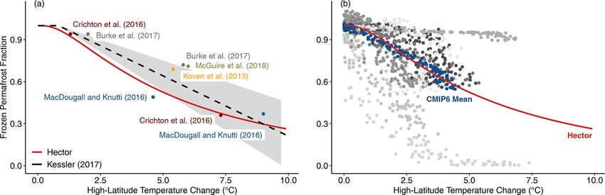
4752                                                     D. L. Woodard et al.: Permafrost in a simple carbon–climate model

shev et al., 2019; Chen et al., 2019). However, the magnitude
of this feedback is still highly uncertain, due to limited data
availability and missing process-based understanding (Burke
et al., 2017, 2020). The potential impact ranges from negligi-
ble to large, with stronger effects possible, particularly over
longer time horizons (Schuur et al., 2015).
   Land surface models, like the Community Land Model
(CLM) and the Joint UK Land Environment Simulator
(JULES), use process-based representations of permafrost
and explicitly model relevant components such as soil heat
flux, soil moisture, hydrology, and vegetation and output
thaw extent and depth, as well as emissions from permafrost
soils (Chadburn et al., 2015; Lawrence et al., 2012). While
high-complexity models benefit from uncertainty quantifica-
tion, they require large numbers of inputs and are compu-          Figure 1. Hector’s default carbon cycle showing fluxes (arrows) be-
tationally expensive, making it difficult to directly carry out    tween each carbon pool. The terrestrial carbon cycle pools can be
uncertainty analysis with these models.                            split into multiple regions, biomes, or other user-defined categories,
   Conversely, simple climate models such as the Model for         so these are shown with multiple boxes. In darker green we show
the Assessment of Greenhouse-gas Induced Climate Change            the addition of our novel permafrost representation in Hector. As
(MAGICC) (Meinshausen et al., 2011) and Hector (Hartin             carbon is exchanged in a variety of forms in Hector, the carbon flux
et al., 2015) sacrifice spatiotemporal resolution and de-          arrows do not correspond to any particular carbon compound except
emphasize process realism in favor of conceptual simplic-          where specified for land emissions. Vegetation, detritus, and soil all
                                                                   emit CO2 , whereas thawed soil produces both CO2 and CH4 emis-
ity and fast execution time. As a result, they can be used
                                                                   sions.
to explore permafrost effects over a wide range of parame-
ters and to analyze the relative significance of various per-
mafrost controls. Similar models have previously been used
to explore permafrost processes such as abrupt thaw that are       global-scale behavior of more sophisticated climate mod-
not yet included in Earth system models (ESMs) (Turetsky           els. Hector’s simplicity and modular design make it easy to
et al., 2020) and to understand structural and parametric un-      change the model’s internal structure, while its fast computa-
certainty (Schneider von Deimling et al., 2015; Chadburn           tion time (∼ 1–2 s) allows for easier interpretation of model
et al., 2017; Koven et al., 2015b). Simple climate models          behavior and facilitates sensitivity and uncertainty analy-
can also be calibrated to emulate the mean global behavior         ses as well as prototyping of new submodules and features.
of Earth system models to a high degree of accuracy (Mein-         Other significant advantages of Hector are its low memory
shausen et al., 2011).                                             requirements, ease of compilation, and optional R interface
   Here, we describe the addition of a permafrost pool and         for setting inputs and parameters and retrieving model out-
a permafrost thaw mechanism to the simple carbon–climate           puts. Here, we focus on Hector’s carbon cycle as relevant
model Hector, with the goal of providing a long-term plat-         to the addition of a permafrost carbon pool; however, for a
form for addressing a suite of science questions. Hector has       detailed description of the structure, components, and func-
been used for a wide range of analyses including climate ef-       tionality of the base version of Hector, the reader is referred
fects on hydropower (Arango-Aramburo et al., 2019), ocean          to Hartin et al. (2015). For subsequent updates, see the Hec-
acidification (Hartin et al., 2016), global building energy use    tor GitHub repository (https://github.com/JGCRI/hector, last
(Clarke et al., 2018), and for exploring the effects of observa-   access: 30 May 2021).
tional constraints on estimates of climate sensitivity (Vega-         Ocean carbon in Hector is exchanged between the atmo-
Westhoff et al., 2019). Including a representation of per-         sphere and four carbon pools that model both physical cir-
mafrost in this model will allow for the consideration of per-     culation and chemical processes in the ocean. Carbon is
mafrost in future such analyses with Hector, and, thanks to        taken up from the atmosphere in the high-latitude surface
Hector’s ability to represent separate biomes or regions, will     box, which transfers some portion of this carbon to the deep
be particularly important for evaluating the specific impacts      ocean carbon pool. Carbon then circulates up to the interme-
of climate change in high latitudes.                               diate ocean layer, to the high- and low-latitude surface pools,
                                                                   and is then outgassed back to the atmosphere from the low-
                                                                   latitude surface pool (Fig. 1).
2   Hector model design                                               Hector’s default terrestrial carbon cycle includes three
                                                                   land carbon pools – vegetation, detritus, and soil – which
Hector (Hartin et al., 2015, 2016) is an open-source, object-      can each be separated across multiple user-defined cate-
oriented simple carbon–climate model that can emulate the          gories (corresponding to, e.g., biomes, latitude bands, or

Geosci. Model Dev., 14, 4751–4767, 2021                                              https://doi.org/10.5194/gmd-14-4751-2021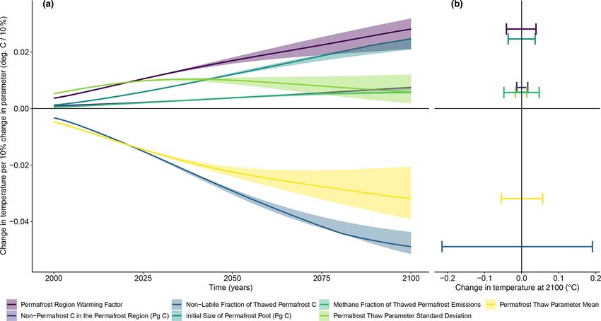
D. L. Woodard et al.: Permafrost in a simple carbon–climate model                                                                 4753

geopolitical units), each with their own set of parameters.       set to 1 by default for all groups but can be adjusted by the
When speaking generally, we will refer to these categories        user:
as “groups” in this text. The vegetation pool takes up car-
                                                                  T [i, t] = wfi · T [t].                                          (6)
bon from the atmosphere as net primary productivity (NPP),
some of which is transferred into the detritus pool, which can    2.1   Permafrost submodel
be decomposed and enter the soil carbon pool. All three land
carbon pools separately emit carbon back to the atmosphere        We added permafrost to Hector as an additional, separate soil
from land use change, and soil and detritus release additional    carbon pool that does not decompose or otherwise interact
carbon through decomposition-driven microbial respiration         with the rest of Hector’s carbon cycle until it thaws. There-
(Fig. 1).                                                         fore, Hector’s land carbon cycle with permafrost includes
   The annual change in atmospheric carbon in Hector, dCdtatm ,   five pools: vegetation, detritus, non-permafrost soil, per-
at time t in units of petagrams of carbon per year is given by    mafrost, and thawed permafrost. Following previous model-
                                                                  ing approaches, we focus on only the top 3 m of permafrost
1Catm                                                             (Kessler, 2017; Koven et al., 2015b), which is also con-
      (t) = FA (t) + FLC (t) − FO (t) − FL (t),            (1)
 dt                                                               sistent with the non-permafrost soil carbon pools in Hec-
                                                                  tor. At each time step, a temperature-controlled fraction of
where FA is the flux of anthropogenic industrial and fos-         permafrost carbon by mass is exchanged between the per-
sil fuel emissions, and FLC is land use change emissions,         mafrost and thawed permafrost carbon pools. In the thawed
both defined as positive to the atmosphere. FO is the             permafrost pool, carbon is available for decomposition into
net atmosphere–ocean carbon flux, and FL is the land–             CO2 and CH4 after subtracting a separately tracked stock of
atmosphere carbon flux, both defined as positive into their       non-labile, or static, carbon in this pool. We define this static
respective pools. FL is defined as NPP (carbon uptake) mi-        carbon fraction within the thawed permafrost pool follow-
nus emissions from heterotrophic respiration (RH) at time t       ing Schädel et al. (2014) as thawed permafrost carbon that
across all n number of user-defined groups:                       is nearly inert and has a turnover time of up to thousands
           n
           X                  n
                              X                                   of years. Carbon moves primarily from the permafrost pool
FL (t) =         NPPi (t) −         RHi (t).               (2)    to the thawed pool as temperatures rise in the future, but re-
           i=1                i=1                                 freeze of thawed carbon is also possible in scenarios where
                                                                  emissions reductions allow for potential cooling.
  Heterotrophic respiration for group i at time t (RH[i, t],         For a permafrost carbon pool at time t, Cperm [t], and a
Pg C yr−1 ) includes contributions from both soil (RHs ) and      thawed permafrost carbon pool, Cthawed [t], (both in units
detritus (RHd ) decomposition, although it only includes          of Pg C), permafrost carbon in Hector is exchanged as fol-
emissions from CO2 , not CH4 :                                    lows:
RH[i, t] = RHs [i, t] + RHd [i, t]                         (3)    Cperm [t] = Cperm [t − 1] − 1Cperm [t]                           (7)
RHd [i, t] = frd Cd Q10 [i]T [i,t]/10                      (4)    Cthawed [t] = Cthawed [t − 1] + 1Cperm [t] − Fthawed-atm ,       (8)
RHs [i, t] = frs Cs Q10 [i]T200 [i,t]/10 .                 (5)    where 1Cperm [t] is the change in the permafrost carbon pool
                                                                  at time t due to permafrost thaw or refreeze, and Fthawed-atm
   Detritus and soil heterotrophic respiration are both pro-      is the flux of carbon (in Pg C) from the thawed permafrost
portional to the sizes of their respective carbon pools (Cd       pool to the atmosphere, including both CO2 and CH4 emis-
and Cs , both in Pg C), with a rate that increases exponen-       sions (see Sect. 2.1.1). Assuming a uniform permafrost car-
tially with temperature according to a group-specific temper-     bon density, 1Cperm [t] is given by
ature sensitivity parameter (Q10 [i]). The corresponding frac-
                                                                  1Cperm [t] = (ffrozen [t] − ffrozen [t − 1]) · Cperm [t − 1],    (9)
tions of respiration carbon, transferred annually, from each
pool are given by frs and frd . Detritus respiration increases    where ffrozen [t] is the mass fraction of permafrost carbon re-
with group-specific air temperature change (T [i, t]), while      maining at time t.
soil respiration increases with the 200-year running mean of         To a first approximation, ffrozen [t] can be estimated as a
air temperature (T200 [i, t]), a somewhat arbitrary choice of     function of mean air temperature (global or adjusted by a
smoothing used in Hector as a proxy for soil temperatures in      group-specific warming factor). We calculate ffrozen at each
Hector’s respiration calculations. This dampens the variabil-     time step in Hector following the model reported by Kessler
ity and produces a slower response in soil warming compared       (2017), but we recalibrated the model to use high-latitude
with air temperatures.                                            temperatures, THL (which are proportional to global temper-
   T [i, t] is the change in annual mean temperature (K) in       atures based on a high-latitude warming factor, wfHL ), in-
group i at time t since the initial model period and is modeled   stead of global mean surface temperatures, and we use a log-
as the globally averaged mean annual temperature, T , at time     normal cumulative distribution function (CDF) instead of a
t multiplied by a group-specific warming factor, wfi , that is    linear model:

https://doi.org/10.5194/gmd-14-4751-2021                                              Geosci. Model Dev., 14, 4751–4767, 2021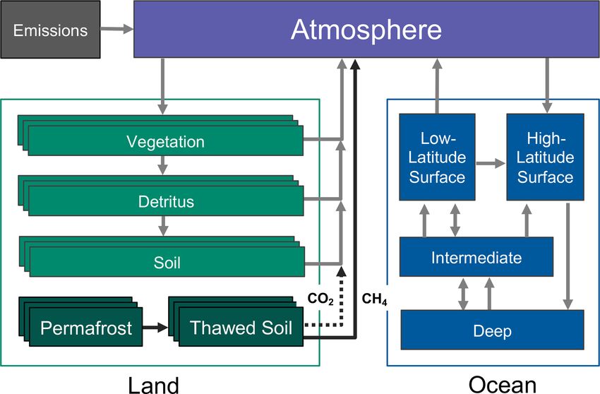
4754                                                      D. L. Woodard et al.: Permafrost in a simple carbon–climate model

ffrozen [t] = 1 − NCDF(log(1THL )|µ, σ )                    (10)    staticc [i, t] = staticc [i, t − 1] + fstatic × 1Cperm [i, t].   (12)
THL [t] = wfHL · T [t],                                     (11)
                                                                        In the case of refreeze, carbon is removed from staticc
where NCDF is the normal cumulative distribution function,          proportional to the amount of static carbon currently in the
and µ and σ are the mean and standard deviation of the log-         thawed permafrost pool. In the interest of computational ef-
normal distribution. These two parameters control the frozen        ficiency, this value is not included as a separate carbon pool
fraction of permafrost as a function of temperature and can be      in Hector; rather, it is simply a variable to track the amount
interpreted as follows: eµ is the temperature at which 50 %         of static carbon within the thawed pool over time.
of the permafrost is thawed, whereas σ controls how sud-                Of the remaining labile carbon in the thawed carbon pool,
den the thaw is around the mean relative to lower and higher        most decomposes aerobically to CO2 from microbial res-
temperatures. Technically, permafrost area could increase in        piration, while a small fraction generates CH4 emissions
the case of cooling temperatures; therefore, the area fraction      from anaerobic respiration. Heterotrophic respiration emis-
could be greater than one. However, because even the most           sions from Hector’s thawed permafrost carbon pool are par-
aggressive climate action scenarios show future temperatures        titioned between CO2 and CH4 based on a CH4 respiration
that stabilize above early 21st century temperatures, we as-        fraction, fCH4 .
sume that permafrost area will never grow more than the                 With the addition of permafrost in Hector, the total het-
starting value.                                                     erotrophic respiration flux of CO2 (RH[i, t]) for group i at
   The lognormal CDF was chosen for several reasons. Its            time t is the sum of heterotrophic respiration in detritus
curvature captures the “activation energy” of permafrost            (RHd ), soil (RHs ), and thawed permafrost (RHpf ):
thaw with respect to temperature for low temperature change
(left side of the curve), and, more importantly, the “dimin-        RH[i, t] = RHs [i, t] + RHd [i, t] + RHpf [i, t].                (13)
ishing returns” of permafrost thaw at higher temperatures
because the more accessible near-surface permafrost has al-            The thawed permafrost CO2 respiration flux, RHpf , is pro-
ready thawed by that point. Additionally, its parameters are        portional to the size of the thawed pool, Cthawed , based on the
readily interpretable in terms of the timing of 50 % per-           static fraction of carbon in that pool, fstatic , and to the fraction
mafrost loss (eµ ) and the rate of permafrost loss around the       of emissions released as CH4 , and increases exponentially
50 % point relative to earlier/later in the process (σ ), which     with the 200-year running mean of temperature, following
facilitates the use of this framework to emulate global per-        the formulation from Hector’s default soil pool.
mafrost dynamics in more complex models. Finally, it is nat-
urally bounded between 0 and 1, which is appropriate as a           RHpf [i, t] =(1 − fCH4 ) · (Cthawed − staticc )
model of the remaining permafrost fraction.                                       · Q10 [i]T200 [i,t]/10                             (14)
   While our tuned lognormal CDF aligns well with previous
model results (see Sect. 2.3), there are a variety of possible         The CH4 respiration flux from thawed permafrost is es-
choices for this functional form, and others can be explored        timated similarly but is added to natural CH4 emissions in
in future model development efforts. Fortunately, the modu-         Hector, which are prescribed at 300 Tg yr−1 (Hartin et al.,
lar design and coding best practices of Hector make it simple       2015) to affect atmospheric CH4 concentrations.
to substitute alternatives for this equation.
                                                                    RHCH4 [i, t] =(fCH4 ) · (Cthawed − staticc )
2.1.1   Permafrost carbon emissions
                                                                                     · Q10 [i]T200 [i,t]/10                          (15)
Even after thaw, only a fraction of permafrost carbon is avail-
able for decomposition. While in reality turnover times of             Thus, the total flux of carbon to the atmosphere from the
soil organic carbon fall anywhere along the range from a few        thawed permafrost pool, Fthawed-atm , is
days to thousands of years (Schädel et al., 2014), we group
                                                                    Fthawed-atm [i, t] = RHCH4 [i, t] + RHpf [i, t].                 (16)
soil decomposition broadly into labile and non-labile pools,
where carbon in the non-labile (static) pool decomposes on             While there are other processes occurring (see Sect. 4)
the order of up to thousands of years and is assumed to be          these are thought to be the major processes controlling
inert for the purpose of this analysis. In Hector, a static frac-   decadal permafrost dynamics (Schuur et al., 2015).
tion of total thawed permafrost carbon, fstatic , is used to de-
termine a separately tracked value of the total static carbon       2.2   Coupled Model Intercomparison Project data
within the thawed permafrost carbon pool (staticc ) at each
time step before decomposition. For group i at time t for all       We used data from Phase 6 of the Coupled Model Inter-
time steps where 1Cperm [i] is positive (permafrost is thaw-        comparison Project (CMIP6) to derive vegetation and litter
ing),                                                               parameters for the permafrost region as well as to validate

Geosci. Model Dev., 14, 4751–4767, 2021                                               https://doi.org/10.5194/gmd-14-4751-2021
D. L. Woodard et al.: Permafrost in a simple carbon–climate model 4755
Table 1. Hector configuration of permafrost-related parameters and initial values based on literature review. Ranges shown are used for the
sensitivity analysis. Cperm (t = 0) was estimated by scaling up 727 Pg C (Hugelius et al., 2014) based on the fraction of permafrost thaw in
CMIP models (Koven et al., 2013). The soil, vegetation, and litter carbon initial values comprise the non-permafrost carbon pools in the
permafrost region, and were estimated from CMIP6 model data and Hugelius et al. (2014). The permafrost thaw parameters µ and σ are
tuned parameters, estimated by optimizing the model against results from Koven et al. (2013) while keeping within the upper and lower
bounds from Kessler (2017).
Hector Estimated
Parameter nomenclature Value range Reference Description
µ pf_mu 1.67 1.43–1.91 Tuned to Kessler (2017) Permafrost thaw parameter
σ pf_sigma 0.99 0.86–1.11 Tuned to Kessler (2017) Permafrost thaw parameter
fstatic fpf_static 0.74 0.4–0.97 Burke et al. (2012, 2013); Static permafrost fraction
Schädel et al. (2014)
Cperm (t = 0) permafrost_c 865 Pg C 740–991 Pg C Estimated from Hugelius Initial permafrost carbon
et al. (2014)
Csoil (t = 0) soil_c 308 Pg C 263–352 Pg C Hugelius et al. (2014) Initial non-permafrost soil C in
the permafrost region
Cveg (t = 0) veg_c 16.5 Pg C 3.17–29.8 Pg C Derived from CMIP6 Initial vegetation C stock in the
model data permafrost region
Clitter (t = 0) litter_c 6.06 Pg C 1.24–10.9 Pg C Derived from CMIP6 Initial detritus C stock in the
model data permafrost region
wf warmingfactor 2.0 1.75–2.25 Meredith et al. (2019) High-latitude warming factor
fCH4 rh_ch4_frac 0.023 0.006–0.04 Schuur et al. (2013); Fraction of thawed permafrost
Nzotungicimpaye and carbon decomposed as CH4
Zickfeld (2017); Schädel
et al. (2016)
our permafrost–temperature curve. Following Burke et al. 2.3 Configuration and tuning
(2020), we include permafrost grid cells above 20◦ N that are
not covered by ice at the start of the historical period. Per- To run Hector with permafrost, we separated the land com-
mafrost is defined by grid cells where the 2-year mean soil ponent of the model into permafrost and non-permafrost
temperature at the depth of zero annual amplitude (Dzaa ) of groups, more intuitively thought of as regions in this con-
ground temperature remains below 0 ◦ C for at least 2 years. text. In the permafrost region all parameters were set to the
In models where the maximum soil depth is less than the values given in Table 1, and we allocated 3 % of the initial
Dzaa , temperature in the deepest available soil layer was global vegetation carbon (equivalent to 17 Pg C) and 11 % of
used. This approximation may result in somewhat underes- the initial detritus carbon (6.1 Pg C) based on the mean share
timating permafrost extent. High-latitude temperatures and of vegetation and litter carbon in permafrost-containing grid
permafrost vegetation and litter values were estimated by cells in CMIP6 models at the end of the historical simula-
masking out non-permafrost grid cells. tion. For the fraction of non-permafrost soil carbon in the
We chose models used in Burke et al. (2020), but sev- permafrost region, we used a value of 13 % of the global
eral of these models did not report the necessary variables non-permafrost soil carbon (equivalent to 308 Pg C, follow-
in the Earth System Grid Federation archive, so we used ing Hugelius et al., 2014). Initial permafrost carbon in Hec-
only ACCESS-ESM1-5, CNRM-ESM2-1, CanESM5, GISS- tor was set to 865 (± 125) Pg C based on the 727 Pg C esti-
E2-1-G, MIROC6, MPI-ESM1-2-HR, MRI-ESM2-0, and mate for near-surface (< 3 m depth) permafrost by Hugelius
NorESM2-LM for comparing our permafrost–temperature et al. (2014) and scaled up based on historical thaw from
relationship (Fig. 2b) and our thaw estimates. Of those mod- Koven et al. (2013) so that the resulting modern value is
els, only NorESM2, CNRM-ESM2-1, ACCESS-ESM1-5, close to 727 Pg C. We did not use the full 1035 Pg C reported
and CanESM5 reported the relevant carbon outputs and were in Hugelius et al. (2014) here, as this includes both frozen
able to be used in estimating vegetation and litter in the per- and non-frozen soil, and we instead allocated the remaining
mafrost region. 308 Pg C to non-permafrost soil in the permafrost region.
https://doi.org/10.5194/gmd-14-4751-2021 Geosci. Model Dev., 14, 4751–4767, 20214756 D. L. Woodard et al.: Permafrost in a simple carbon–climate model We also amplified warming in the permafrost region as a 2014), we make the simplifying assumption that the CH4 constant multiple of global mean temperatures in Hector, to fraction of overall emissions is static over time. As further account for increased rates of warming at high latitudes. We estimates of this relationship are published, we can update set this warming factor, wfHL , to 2.0 (Meredith et al., 2019). our model parameterization. We used the upper and lower bounds (± 1 standard error from the best estimate in Kessler, 2017) to recalibrate the 2.4 Evaluation model in Kessler (2017) to high-latitude temperatures and then fitted our lognormal distribution parameters µ and σ to We ran Hector with and without permafrost feedbacks us- the upper and lower bounds of this adjusted model version. ing forcings from each of four Representative Concentration Following this, we used these parameter ranges to tune the Pathways (RCPs): RCP2.6, RCP4.5, RCP6.0, and RCP8.5 permafrost module against CMIP5 multi-model mean output, (Moss et al., 2010). We chose these scenarios to broadly using the “L-BFGS-B” method from the optim function in demonstrate the impacts of a wide range of future climate the R stats package. We tuned based on the fraction of conditions on permafrost thaw and permafrost-driven car- permafrost remaining over the period from 1850 to 2005 and bon emissions and for ease of comparison with other results. from 2005 to 2100 in RCP4.5 and RCP8.5, as reported in The only difference between our model runs with and with- Koven et al. (2013). Our tuned permafrost thaw–temperature out permafrost feedbacks is that the baseline (no-permafrost) relationship aligns well with previous analyses and CMIP6 configuration of Hector is initialized with Cperm (t = 0) set to data (Fig. 2). We note that thaw fractions derived from our 0 to turn off permafrost feedbacks. Our analysis focused on analysis of CMIP6 model results are not substantially differ- the 21st century, but we also show some longer-term effects ent from CMIP5, as also found by Burke et al. (2020), and of permafrost out to 2300. Hector has not been calibrated tuning to these instead affected our permafrost thaw parame- over this period, however, and these findings should be taken ter values by less than 0.1 %. as provisional. We also ran the model with and without ac- Our tuned model results closely aligned with the findings tive CH4 emissions to estimate the separate contributions of in Koven et al. (2013) and gave us a modern permafrost car- permafrost-driven CO2 and CH4 emissions to the permafrost bon value very close to that in Hugelius et al. (2014) (Ta- carbon feedback. ble 2). The final tuned value of σ that we used as our default Given that much uncertainty remains surrounding per- baseline in this analysis was 0.986, whereas the tuned value mafrost controls, we evaluated the sensitivity of the model to of µ was 1.67, which is at the lowest end of the range we used changes in several of the permafrost-specific controls avail- for tuning. To give a more intuitive sense of this number, eµ , able in Hector across their estimated ranges from the litera- or 5.3 ◦ C, corresponds to the high-latitude temperature dif- ture (Table 1). The parameters that we include are the per- ference since preindustrial at which only 50 % of all shallow mafrost thaw parameters µ and σ , the initial size of the shal- permafrost will remain. low permafrost pool available for thaw (Cperm (t = 0)), the Estimates of the fraction of static carbon (not vulnerable to fraction of thawed permafrost that is not available for decom- decomposition) vary widely and still have a high uncertainty position (fstatic ), the warming factor used in the permafrost (Kuhry et al., 2020), but we use a mean of 0.74 (0.4–0.97) region (wfHL ), and the fraction of thawed permafrost carbon based on estimates by Schädel et al. (2014) with the upper emissions that decomposes to CH4 (fCH4 ). We additionally bound derived from the same analysis and a lower bound include a combined value of the total non-permafrost carbon from the best estimate given in earlier work by Burke et al. (nonpfc ) in the permafrost region across the soil, vegetation, (2012, 2013), which overall found a far smaller static frac- and litter pools. The respective fractions of each pool are de- tion. rived for each value of nonpfc based on a linear fit of their The partitioning between CH4 and CO2 emissions from mean, upper, and lower bound shares. thawed permafrost carbon systems has limited estimates We generated priors for our sensitivity analysis using nor- available in the literature (Dean et al., 2018) and is fairly mal distributions centered on the default values of each pa- uncertain (Schädel et al., 2016; Schuur et al., 2013). It also rameter from Table 1 with standard deviations taken as the depends on soil drainage and anoxia, neither of which are mean difference between the default value and the upper and explicitly modeled in Hector, and it may be substantially af- lower bounds. We then ran Hector with 500 parameter sets fected by abrupt thaw processes (Dean et al., 2018; Turet- randomly sampled from the prior distributions and forced sky et al., 2020). For our default parameterization, we set the with RCP4.5 emissions. We focused on three key climate share of CH4 to be 2.3 % (0.6 %–4 %) of total emissions. The and carbon cycle outcomes: temperature anomalies and at- default value that we chose is based on expert assessment in mospheric CO2 and CH4 concentrations. Based on the ef- Schuur et al. (2013), and the range is from a meta-analysis fects on each outcome in 2100, we estimated the coefficient of incubation data (Schädel et al., 2016) and a recent review of variation, elasticity, and partial variance of each parameter. on the contribution of CH4 to the permafrost feedback (Nzo- Briefly, the coefficient of variation describes the uncer- tungicimpaye and Zickfeld, 2017). While the CH4 fraction is tainty in the parameter (calculated as the parameter variance also known to vary with temperature (Yvon-Durocher et al., divided by the mean), the elasticity describes the sensitivity Geosci. Model Dev., 14, 4751–4767, 2021 https://doi.org/10.5194/gmd-14-4751-2021
D. L. Woodard et al.: Permafrost in a simple carbon–climate model 4757
Figure 2. (a) Lognormal permafrost–temperature relationship (red) in Hector with µ = 1.67 (eµ =5.3) and σ = 0.986, compared with our
high-latitude temperature-adjusted form of the linear model in Kessler (2017) (black). The shaded area shows the upper and lower bounds
given by ± 1 standard deviation from our adjusted version of the best estimate model in Kessler (2017). Additional labeled points show
results from previous modeling studies for comparison. (b) Hector permafrost–temperature relationship (red) shown against CMIP6 data
from individual models (shades of gray) and the mean of the models shown (blue).
Table 2. Values used for tuning Hector’s parameters (column 4) compared against results from Hector after tuning (column 5). The modern
permafrost value in Hector was taken from the year 2010. Koven et al. (2013) values are from the top 50 % of CMIP5 models reported in that
analysis based on the accuracy of modern permafrost area. As we do not consider deep permafrost in the model, values for the remaining
permafrost area in each time period only include permafrost at less than 3 m depth.
Scenario Source Variable Value Hector
– Hugelius et al. (2014) Modern permafrost carbon 0–3 m (Pg C) 727 730
RCP4.5 Koven et al. (2013) Remaining permafrost area 1850–2005 (%) 84 85
RCP4.5 Koven et al. (2013) Remaining permafrost area 2005–2100 (%) 58 56
RCP8.5 Koven et al. (2013) Remaining permafrost area 2005–2100 (%) 29 32
of the model to a relative change in the parameter, and the each parameter, making for simpler computation and easier
partial variance synthesizes these two metrics to describe the interpretation.
relative contribution of uncertainty in a parameter to the total We also visualized the sensitivity of the model to parame-
predictive uncertainty in the model output (i.e., the parame- ter changes more concretely by estimating temperature sen-
ters that have the highest partial variance are those that are sitivity in Hector to unit changes in each parameter over this
highly uncertain and to which the model is highly sensitive; century, and the net effect on temperature in 2100 of varying
parameters that are highly uncertain but to which the model each parameter across its full range (Table 1) in all RCPs.
is relatively uncertain, and conversely, parameters to which This was estimated by running Hector with parameter val-
a model is highly sensitive but whose values are known pre- ues uniformly sampled across each parameter’s range while
cisely, would both have low partial variance). holding all other parameters at their default values. This ne-
We generally followed the approach of LeBauer et al. glects potential interactive effects but, nonetheless, provides
(2013), which sampled from parameter distributions to gen- useful insights about the impact of our parameter choices and
erate an ensemble of model runs that approximate the pos- their uncertainty on our results.
terior distribution of model output that can be used in the
sensitivity analysis. The sensitivity analysis is based on uni-
variate perturbations of each parameter of interest, and the 3 Results
relationship between each parameter and model output is ap-
proximated by a natural cubic spline. The model sensitivity This Hector implementation of permafrost thaw and loss re-
is then based on the derivative of the spline at the parameter produced the magnitude and general temporal trajectory of
median. In our analysis, instead of a cubic spline, we used a globally averaged permafrost thaw simulated by ESMs and
multivariate generalized additive model regression. This al- by simpler permafrost thaw models (Koven et al., 2015a;
lowed us to calculate partial derivatives across the median of Burke et al., 2017; Schuur et al., 2015; McGuire et al.,
2018). In RCP4.5, RCP6.0, and RCP8.5, permafrost losses,
including both thawed permafrost and permafrost carbon
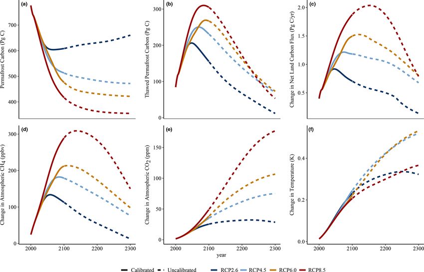
https://doi.org/10.5194/gmd-14-4751-2021 Geosci. Model Dev., 14, 4751–4767, 20214758 D. L. Woodard et al.: Permafrost in a simple carbon–climate model Figure 3. Effect on key climate and carbon outputs of including permafrost in Hector, shown as the difference between a model run with and without active permafrost processes under the default model configuration across RCP2.6, RCP4.5, RCP6.0, and RCP8.5. Results are shown through 2100 (solid lines) as the calibrated period of Hector but are extended to 2300 (dashed lines) to illustrate potential long-term dynamics. The net land carbon flux is the sum of the land–atmosphere carbon fluxes – soil, detritus, and thawed permafrost respiration fluxes of CO2 , thawed permafrost CH4 emissions, land use change, and net primary productivity – and is defined as positive into the atmosphere. that has been decomposed and emitted to the atmosphere, which showed a peak increase of between 1 and 1.5 Pg yr−1 reached 350–450 Pg C by 2100, with the rate of thaw being in RCP8.5, and closer to 0 in RCP4.5 and RCP2.6. This fastest over the 21st century and slowing thereafter (Fig. 3a). somewhat offset the existing land sink over the 21st cen- RCP2.6 is unique in that strong emissions mitigation in this tury, reducing it by between 30 and 60 %. By 2300, the scenario led to cooling temperatures, which allowed for per- influence of permafrost on this flux had dropped to closer mafrost recovery (i.e., refreeze of carbon from the thawed to 1 Pg C yr−1 (Fig. 3c). The inclusion of permafrost in the permafrost pool) to begin by the end of the century in Hector. model had almost no effect on the land–atmosphere flux In all scenarios, the thawed permafrost carbon pool increased purely from non-permafrost C pools. to a peak between the middle and the end of the 21st cen- We found that including CH4 emissions (set to the de- tury, after which losses to CH4 and CO2 from heterotrophic fault fraction of 2.3 % of emissions) in the model resulted respiration began to outpace the carbon inputs from new per- in a 24 %–29 % increase in the effect of the permafrost feed- mafrost thaw. Thawed permafrost carbon stocks were limited back on global mean temperatures, adding around 0.06 ◦ C of in their ability to decompose fully over longer timescales by warming by 2100 across the RCPs. The relatively short life- the labile fraction, although refreeze removed static and la- time of CH4 in the atmosphere (estimated as 9.1 years by bile carbon alike from this pool in RCP2.6. Stocker et al., 2013) means that the effects of the permafrost The influence of permafrost on the net land–atmosphere carbon feedback on atmospheric CH4 concentrations across carbon flux in Hector was strongest while respiration emis- the RCPs followed a similar trajectory to that of thawed per- sions from permafrost thaw were at their peak, after 2100, re- mafrost carbon, although lagged by several years. As the sulting in a maximum increase of around 2 Pg C yr−1 , some- thawed permafrost carbon pool shrank and CH4 emissions what higher than previous findings in Burke et al. (2017) from this pool declined, permafrost-driven changes in atmo- Geosci. Model Dev., 14, 4751–4767, 2021 https://doi.org/10.5194/gmd-14-4751-2021
D. L. Woodard et al.: Permafrost in a simple carbon–climate model                                                                            4759

Table 3. Permafrost results across all RCP scenarios at 2100 for several key carbon and climate outputs. All results are global and summed
across permafrost and non-permafrost regions. The “total” columns are generated by running Hector with the configuration in Table 1, and
the “change” columns give the percent change from a baseline model run without active permafrost.

                                                                                        Scenario
                                                   RCP2.6                    RCP4.5                    RCP6.0                    RCP8.5
  Output                                   Total     Change (%)      Total     Change (%)      Total     Change (%)      Total     Change (%)
  Permafrost carbon (Pg C)                608.5             −26.2    512.8            −37.8    476.1            −42.3    417.0            −49.5
  Net permafrost CO2 emissions (Pg C)     100.9             100.0    120.6            100.0    121.6            100.0    142.3            100.0
  Change in atmospheric CO2 (ppm)         408.4               6.6    539.4              6.9    686.8              5.9    943.8              5.5
  Net permafrost CH4 emissions (Pg C)       2.4             100.0      2.8            100.0      2.9            100.0      3.4            100.0
  Change in atmospheric CH4 (ppbv)       1300.1               9.5   1841.5             10.8   2000.1             11.9   4581.5              6.7
  Non-permafrost soil carbon (Pg C)      1856.6               0.6   1916.9              0.5   1952.0              0.4   1960.9              0.3
  Detritus carbon (Pg C)                   60.6               1.3     63.8              1.1     66.4              0.8     68.5              0.6
  Vegetation carbon (Pg C)                571.5               1.6    608.6              1.5    629.8              1.2    667.7              1.2
  Temperature anomaly (◦ C)                 1.8              14.5      2.8              9.5      3.4              7.0      4.9              4.4

spheric CH4 also dropped off over the 22nd and 23rd cen-                 was thawed by 2100 when all permafrost parameters were set
turies (Fig. 3b, d). The much longer lifetime of atmospheric             to their default values from Table 1. Between 2000 and 2100
CO2 (300 to 1000 years; Stocker et al., 2013) meant that the             this newly available carbon moved from the thawed pool to
permafrost-driven increases remained over the entire model               the atmosphere and then into the ocean and non-permafrost
run time, long after emissions from the thawed permafrost                land carbon pools (Fig. 4). In RCP8.5, 32 % (146 Pg C) was
began to decline. By 2100, permafrost emissions increased                decomposed and emitted to the atmosphere as CO2 and CH4
atmospheric CO2 by between 25 and 50 ppm across all RCPs,                by the end of the century. Of that 32 %, around 100 Pg C
and by 2300, in all but RCP2.6, the permafrost-driven in-                remained in the atmosphere, 23 Pg C was taken up by the
crease in CO2 concentrations had substantially grown to be-              ocean, 6 Pg C was taken up by the non-permafrost soil, and
tween 75 and 177 ppm.                                                    8 Pg C was taken up by vegetation pools. The effect on the
   Permafrost emissions also drove a steady increase in tem-             detritus pool was less than 1 Pg C. Over longer timescales,
perature over the 21st century, continuing to increase through           the fraction of thawed permafrost carbon emitted to the at-
2300, again in all scenarios but RCP2.6. Consistent with pre-            mosphere through respiration grew to nearly 90 % by 2300,
vious findings (e.g., Burke et al., 2017; MacDougall et al.,             although similar proportions of the permafrost-driven car-
2012, 2013), the influence of permafrost on temperature re-              bon release (here including both permafrost carbon and net
sulted in relatively similar effects on absolute temperatures            carbon losses from non-permafrost soils) were taken up by
across all RCPs this century (Fig. 3f – an increase of be-               Hector’s other carbon pools. The higher temperatures also
tween 0.2 and 0.24 ◦ C by 2100). This meant that the effect              drove net losses in non-permafrost soil carbon by 2300 rel-
was relatively less significant in higher-emissions scenarios,           ative to a model run without permafrost, which is included
declining from a 15 % increase in RCP2.6 to a 4 % increase               here with the permafrost carbon in the calculations involv-
in RCP8.5 at 2100 (Table 3). Over longer timescales the tem-             ing non-permafrost carbon pools as Hector does not currently
perature effects grow more distinct by scenario; the high-               have a meaningful way to evaluate carbon sources within a
est absolute permafrost-driven increases in warming were                 pool (Fig. 4).
in RCP4.5 and RCP6.0 (0.52 and 0.53 ◦ C in 2300, respec-                    While scenarios with lower radiative forcing thawed less
tively), leaving RCP8.5 as only the third highest beyond                 permafrost carbon overall, a somewhat higher fraction of
2250 (Fig. 3f), although total temperature change in Hec-                that carbon ended up released into the atmosphere (40 % by
tor was still highest in RCP8.5. This is due to reductions in            2100 and 94 % by 2300 in RCP2.6). Relatively more of the
the effect of additional carbon emissions on radiative forc-             permafrost-driven carbon release was also taken up by the
ing at higher atmospheric carbon concentrations in the model             ocean in this scenario (26 % by 2100 and nearly 60 % by
(Hartin et al., 2015). These temperature changes found by our            2300) thanks to lower mean global temperatures increasing
model are similar to those in several previous studies (Mac-             the solubility of CO2 in seawater, while 53 % (54 Pg C) re-
Dougall et al., 2012; Burke et al., 2017) (see Sect. 4.2).               mained in the atmosphere by 2100 (31 % by 2300; Fig. 4).

3.1   Permafrost effects on carbon pools                                 3.2     Model sensitivity to permafrost parameters

Across the four RCP scenarios, between 259 and 458 Pg C                  Based on the effects on end-of-century temperature change
(in RCP2.6 and RCP8.5, respectively) of permafrost carbon                and atmospheric CO2 and CH4 concentrations, we found that

https://doi.org/10.5194/gmd-14-4751-2021                                                       Geosci. Model Dev., 14, 4751–4767, 2021
4760 D. L. Woodard et al.: Permafrost in a simple carbon–climate model
Figure 4. Changes in carbon stocks in a permafrost-active model run compared to a run without permafrost at 2050, 2100, and 2300 across
all RCPs. The sum of each bar is the total carbon lost from the permafrost pool by that year in each RCP. Results for 2300 should be taken as
provisional because Hector is not calibrated over this period. While more carbon moves from the thawed pool into the atmosphere and then
into the ocean across the three periods shown, a relatively larger fraction of carbon remains in the atmosphere in higher-warming scenarios.
the most significant permafrost control in Hector was the varied the most across the RCPs. Temperature exhibited the
static fraction, which supports similar findings by previous strongest positive sensitivity to changes in the high-latitude
studies (Koven et al., 2015a; MacDougall and Knutti, 2016). warming factor and initial size of the permafrost carbon pool
This accounted for 68 % of the partial variance in tempera- (0.03 ◦ C 10 %−1 and 0.02 ◦ C 10 %−1 , respectively).
ture (around 30 % in CH4 and 72 % in CO2 ) across all three In practical terms, the effects of varying the static frac-
outcomes (Fig. 5). The second most significant parameter in tion over its plausible range (Table 1) on permafrost-driven
terms of temperature was the initial permafrost carbon value, temperature change spanned nearly 0.4 ◦ C by 2100 across all
which accounted for 10 % of the partial variance, followed RCPs, or up to a 0.2 ◦ C impact compared with the default
by the mean thaw parameter (µ, 9 %). The CH4 fraction and value (Fig. 6b). At the extremes of their potential ranges, the
high-latitude warming factor had small effects (6 % and 7 %, permafrost thaw parameter µ, the high-latitude warming fac-
respectively), while varying the standard deviation thaw pa- tor, the initial size of the permafrost pool, and the CH4 frac-
rameter (σ ) and the initial non-permafrost carbon in the per- tion each had net effects of between +0.04 and +0.06 ◦ C
mafrost region across their ranges had almost no impact on compared with a run at their default values. Consistent with
any output variable. The effect of the CH4 fraction was much our findings in Fig. 5, the non-permafrost carbon and per-
more significant in terms of its effects on atmospheric CH4 mafrost thaw parameter σ had only a minimal impact on
(59 %) but had no discernible effect on CO2 concentrations. temperature when varied over their ranges, around 0.01 ◦ C
Over longer timescales (out to 2300), the influence of the each.
warming factor increased somewhat, whereas the influence
of the CH4 fraction on temperature decreased to nearly zero,
which follows from the decline in permafrost-driven changes 4 Discussion and conclusions
in atmospheric CH4 by this time (Fig. 3).
The temperature response of the model to a unit increase Including permafrost in Hector significantly increased end-
in each parameter generally strengthened over time, with the of-century atmospheric CO2 , CH4 , and warming, although
exception of the permafrost thaw parameter σ which had a the impact on atmospheric CH4 was declining somewhat by
larger impact early on before declining to a sensitivity of the end of the model run. The parameter with the most sig-
0.006 ◦ C 10 %−1 (Fig. 6a). Varying the static fraction caused nificant effects on these outcomes was the fraction of per-
the strongest temperature response, a ∼ 0.04 ◦ C decrease in mafrost not available for decomposition, or the static frac-
temperature for every 10 % increase in fstatic at 2100. The tion. This suggests that further research constraining this pa-
permafrost thaw parameter µ had the next strongest sensi- rameter continues to be important for reducing uncertainty in
tivity by the end of this century, −0.03 ◦ C 10 %−1 , and also permafrost estimations moving forward. While other studies
have supported this finding (MacDougall and Knutti, 2016;
Geosci. Model Dev., 14, 4751–4767, 2021 https://doi.org/10.5194/gmd-14-4751-2021D. L. Woodard et al.: Permafrost in a simple carbon–climate model 4761 Figure 5. Sensitivity analysis of the effect of key permafrost controls on end-of-the-century atmospheric CH4 (orange) and CO2 (gray) con- centrations as well as temperature anomalies (dark red), following LeBauer et al. (2013) and forced with RCP4.5 emissions. The coefficient of variation is the ratio between the input parameter mean and variance, and it reflects the parameter’s relative uncertainty; elasticity is the normalized sensitivity of the model to a change in a particular parameter; and the partial variance, or the fraction of variance in the model output that is explained by the given parameter, integrates the elasticity and coefficient of variation to give the overall sensitivity of the model to each parameter. Figure 6. Sensitivity of temperature over the 21st century across RCP2.6, RCP4.5, RCP6.0, and RCP8.5 to variations in each of the key permafrost parameters in the model. Panel (a) shows the sensitivity of temperature in Hector to unit changes in each parameter from its default value, and how that sensitivity varies over time and by emissions scenario. Shaded regions correspond to the range across RCP2.6, RCP4.5, and RCP8.5, and the solid line shows the median. Panel (b) gives the total effect on temperature in 2100 from varying each parameter across its potential range – in other words, how the potential sensitivities in panel (a) translate to practical effects at the end of the century based on the actual ranges of each parameter. https://doi.org/10.5194/gmd-14-4751-2021 Geosci. Model Dev., 14, 4751–4767, 2021
4762                                                     D. L. Woodard et al.: Permafrost in a simple carbon–climate model

Koven et al., 2015a), it is still important to acknowledge that    soils (Elberling et al., 2013). Thawing permafrost itself im-
the significance of any parameters in Hector is limited by the     pacts soil moisture, although predicting these effects is diffi-
simplicity of the permafrost representation that we are able       cult (Wickland et al., 2006). Moisture also affects the balance
to include and may change with more detailed, physically           of aerobic and anaerobic decomposition, determining the ra-
based representations of the processes involved.                   tio of CO2 to CH4 release (Turetsky et al., 2002). For exam-
                                                                   ple, Lawrence et al. (2015) found that permafrost thaw in-
4.1    Model limitations                                           creased soil drying, reducing the CH4 fraction of permafrost
                                                                   emissions to the extent that the global warming potential of
While we attempted to use reasonable values for our model          emissions from the permafrost region was reduced by 50 %.
parameters and calibrated Hector to emulate the behavior           Projections of drying soils due to permafrost thaw are also
of permafrost thaw in global climate models, these results         supported by the analysis in Andresen et al. (2020).
should be taken as demonstrative of this model’s capabilities,        Hector’s permafrost module also only accounts for carbon
rather than conclusive projections, as model parameter values      stored in the top 3 m of soil, as this shallow permafrost is the
can be adjusted as needed to reflect the latest understanding      most vulnerable to both thaw and decomposition (Kessler,
of permafrost characteristics, and this was not our focus here.    2017). However, an analysis accounting for abrupt thaw
It is more important to acknowledge the permafrost dynam-          found higher contributions from deep carbon when including
ics that are not captured in this model’s structure.               these abrupt thaw processes (Schneider von Deimling et al.,
   Hector’s permafrost module parameterizes gradual per-           2015; Anthony et al., 2018). Previous modeling results have
mafrost thaw, following previous development on simple cli-        found that ∼ 2 Pg C may be emitted over the next century
mate models (Kessler, 2017), but leaves off consideration of       from this deeper permafrost (Koven et al., 2015b), or an ad-
abrupt thaw, which has been found to be a potentially sig-         ditional 3 % of total permafrost-driven carbon emissions over
nificant contributor to future permafrost emissions (Turetsky      that time period, but this study also neglected abrupt thaw
et al., 2020), increasing the overall permafrost soil carbon       processes. There may also be a larger contribution from this
emissions by 125 %–190 % above that from gradual thaw              pool over longer-term results as warming would have more
and increasing the contribution of CH4 to those emissions,         time to reach these deposits, although warming in Hector lev-
according to a recent analysis (Anthony et al., 2018). Abrupt      els off beyond the end of the century.
thaw is also missing from current Earth system models, so             While other mechanisms are included in ESMs, and some
our tuning to these models would not account for this mech-        of their effects on permafrost thaw can be implicitly captured
anism, and it may mean that Hector is somewhat under-              through calibration, not explicitly modeling these effects can
estimating the permafrost carbon feedback. Abrupt thaw is          still impact temporal dynamics and the relative strength of
also a key process for permafrost in peatland soils, and a re-     particular outcomes. A key difference between Hector and
cent analysis estimates an additional 40 Pg of permafrost car-     ESMs is spatial representation. While ESMs are spatially
bon stored in peat than had been found previously (Hugelius        explicit, Hector is primarily global, although with separate
et al., 2020). Based on our sensitivity analysis, increasing the   calculations for land regions or other groups. In the case of
initial permafrost by this amount might translate to around a      the results shown here, only a single permafrost category
0.02 ◦ C increase in overall temperature change by 2100.           was used; this combines high-latitude and high-elevation per-
   Thawing permafrost, particularly abrupt thaw processes,         mafrost, although in reality these may be differently affected
can affect geometry and drainage patterns of the landscape,        by climate. Future analyses with this model may choose to
including creating thaw lakes which are persistent sources         further subdivide the permafrost region into more specific
of both CH4 and CO2 (Vonk et al., 2015; Matveev et al.,            categories to better address these different dynamics.
2016). Hector does not include hydrological processes nor             We also made the simplifying assumption that thawed per-
abrupt thaw mechanisms that could account for this effect,         mafrost carbon does not interact with the vegetation or detri-
and this additional consequence of permafrost thaw on emis-        tus pools, and that newly thawed permafrost carbon does not
sions would not have been captured through tuning to CMIP          affect the potential size of the vegetation and detritus pools
models because we only tuned Hector against the fraction           in the permafrost region. This means that our results exclude
of permafrost thaw in each. While we found that permafrost         any potential changes in plant productivity as a result of per-
emissions from Hector’s thawed pool dropped over time as           mafrost thaw, including any due to changes in nutrient avail-
thaw slowed and the thawed pool decomposed, the model is           ability, although the sign of these effects is highly uncertain
missing this longer-term affect of permafrost thaw on CH4          (Frost and Epstein, 2014; Li et al., 2017).
and CO2 emissions in the region.                                      An additional area of focus for future work should be Hec-
   The absence of hydrological processes in Hector also            tor’s handling of heterotrophic respiration in soil, which cur-
means the model misses interactions between permafrost             rently uses a fairly arbitrary 200-year running mean of air
thaw and soil moisture. Soil moisture has been found to play       temperature as a proxy for soil temperature. This controls soil
a critical role in the rate of release of thawed permafrost car-   decomposition and, thus, climate effects in Hector, including
bon, as drier soils release carbon much faster than wetter

Geosci. Model Dev., 14, 4751–4767, 2021                                            https://doi.org/10.5194/gmd-14-4751-2021
D. L. Woodard et al.: Permafrost in a simple carbon–climate model 4763
Table 4. Comparison of Hector’s results to values from previous studies. As Hector does not account for permafrost in terms of area, we
estimated the values for comparison to McGuire et al. (2018) based on the fraction of permafrost lost over this time period, multiplied by the
initial permafrost area in McGuire et al. (2018).
Scenario Source Variable Value Hector
RCP8.5 Burke et al. (2020) Permafrost remaining 2005–2100 (%) 37 32
RCP4.5 McGuire et al. (2018) Permafrost lost 2010–2299 (× 106 km2 ) 4.1 7.4
RCP8.5 McGuire et al. (2018) Permafrost lost 2010–2299 (× 106 km2 ) 12.7 12.2
RCP4.5 MacDougall and Knutti (2016) Cumulative permafrost CO2 emissions 1850–2100 (Pg C) 71 121
RCP8.5 MacDougall and Knutti (2016) Cumulative permafrost CO2 emissions 1850–2100 (Pg C) 101 142
RCP8.5 Schuur et al. (2015), Cumulative permafrost CO2 emissions 2010–2100 (Pg C) 92, 130.9
Koven et al. (2015) 28–113
– Kirschke et al. (2013) Permafrost CH4 flux 2010 (Tg C yr−1 ) 30 20.7
RCP8.5 Koven et al. (2015) Permafrost CH4 flux change 2010–2100 (Tg C yr−1 ) 3.97–10.48 59
RCP8.5 Knoblauch et al. (2018) Relative mineralization of 22 5.7
permafrost C 2010–2100 (g CH4 kg C−1 )
RCP8.5 Crichton et al. (2016), Permafrost-driven temperature change by 2100 (%) 10–40, 4.4–14.5
Burke et al. (2017) 0.2–12
RCP8.5 MacDougall et al. (2012) Permafrost-driven temperature change by 2100 (◦ C) 0.27 0.21
from permafrost, and should be further evaluated against al- (Table 4). The fraction of permafrost remaining in Hector in
ternative functional forms. RCP8.5 by 2100 aligns fairly closely with the results from
Finally, we do not include any insulating effect from snow CMIP6 models estimated by Burke et al. (2020). Even during
and vegetation, which can protect permafrost from warmer the uncalibrated period of Hector, the land area of permafrost
air temperatures (Shur and Jorgenson, 2007). However, this lost still compares well against estimates from McGuire et al.
effect may be small on the global scale, as including such (2018) in RCP8.5, although not as well in RCP4.5.
protected permafrost was not found to substantially alter the Cumulative permafrost CO2 emissions by 2100 were gen-
amount of permafrost thaw over the next century of warming erally higher than previous results in both RCP4.5 and
according to a 2017 analysis by Chadburn et al. (2017), al- RCP8.5 (MacDougall and Knutti, 2016; Schuur et al., 2015;
though this analysis used equilibrium temperatures and does Koven et al., 2015b). The values given in Schuur et al. (2015)
not give us information about the potential for these insula- include the entire permafrost profile rather than 0–3 m as is
tion effects to play a role in mitigating transient thaw. represented in Hector, which implies an even stronger differ-
Of these limitations, we consider the most significant and ence between these results and Hector’s.
likely influential on the magnitude of our results to be the The modern CH4 flux in Hector was around 30 % lower
lack of abrupt thaw processes, including the effects of abrupt than that found by Kirschke et al. (2013), and Hector’s cumu-
thaw on deeper permafrost carbon. Results from Anthony lative CH4 emissions from 2010 to 2100, normalized by the
et al. (2018) suggest that our model may be underestimat- initial permafrost pool size, were much lower than a more re-
ing the permafrost carbon feedback by as much as 20 %– cent estimate from incubation data (Knoblauch et al., 2018).
50 %, although there are still only limited estimates of these However, the increase in the CH4 flux the by the end of the
effects in the literature. The other significant effect on per- century was substantially higher in Hector compared with es-
mafrost emissions estimates in Hector is the lack of hydro- timates by Koven et al. (2015b). The CH4 contribution to
logical processes, which would potentially generate longer- permafrost-driven temperature change estimated by Hector
term increases in emissions from permafrost thaw due to lake was between 24 % and 29 %, somewhat higher than the 16 %
formation. Other mechanisms affecting rates of permafrost given in Schaefer et al. (2014), but just under the 30 %–50 %
thaw are included in CMIP models; thus, we expect to have range given by the expert assessment in Schuur et al. (2013).
captured the net end-of-century effects of these mechanisms Previous estimates of the temperature amplification of per-
through tuning to CMIP outputs. mafrost carbon feedback by the end of the century cover a
wide range: from 0.1 to 0.8 ◦ C in MacDougall et al. (2012)
4.2 Comparison to previous work with a best estimate of 0.27 ◦ C, from 10 % to 40 % of peak
temperature change in Crichton et al. (2016), and from 0.2 %
While our permafrost model is necessarily limited in com- to 12 % of peak temperature change in Burke et al. (2017).
plexity by Hector’s structure and by the need for computa- In Hector, we find a temperature amplification due to per-
tional efficiency, we are able to reasonably reproduce previ- mafrost emissions of 4 %–15 %, or around 0.2 ◦ C, by 2100
ous results from both simple and more sophisticated models across all four RCPs (Table 3), which falls close to the best
https://doi.org/10.5194/gmd-14-4751-2021 Geosci. Model Dev., 14, 4751–4767, 2021You can also read