Deep desiccation of soils observed by long-term high-resolution measurements on a large inclined lysimeter - HESS
←
→
Page content transcription
If your browser does not render page correctly, please read the page content below
Hydrol. Earth Syst. Sci., 25, 3519–3538, 2021
https://doi.org/10.5194/hess-25-3519-2021
© Author(s) 2021. This work is distributed under
the Creative Commons Attribution 4.0 License.

Deep desiccation of soils observed by long-term high-resolution
measurements on a large inclined lysimeter
Markus Merk, Nadine Goeppert, and Nico Goldscheider
Institute of Applied Geosciences (AGW), Karlsruhe Institute of Technology (KIT), Kaiserstr. 12, 76131 Karlsruhe, Germany

Correspondence: Markus Merk (markus.merk@kit.edu)

Received: 5 June 2020 – Discussion started: 2 July 2020
Revised: 31 March 2021 – Accepted: 12 April 2021 – Published: 22 June 2021

Abstract. Availability of long-term and high-resolution mea-      1   Introduction
surements of soil moisture is crucial when it comes to un-
derstanding all sorts of changes to past soil moisture varia-     The understanding of soil moisture dynamics and its cou-
tions and the prediction of future dynamics. This is particu-     pling to climate and climate change is crucial when it comes
larly true in a world struggling against climate change and       to predictions of future variability of soil moisture storage
its impacts on ecology and the economy. Feedback mech-            and exchange with the atmosphere and vegetation. Long-
anisms between soil moisture dynamics and meteorologi-            term data sets of measured soil moisture are of critical im-
cal influences are key factors when it comes to understand-       portance to achieve a better understanding of how these sys-
ing the occurrence of drought events. We used long-term           tems interact and to identify the main drivers for seasonal
high-resolution measurements of soil moisture on a large in-      and long-term soil moisture variations. Drought and feed-
clined lysimeter at a test site near Karlsruhe, Germany. The      back mechanisms between soil moisture and extreme tem-
measurements indicate (i) a seasonal evaporation depth of         peratures are documented in the literature (Lanen et al., 2016;
over 2 m. Statistical analysis and linear regressions indicate    Perkins, 2015; Samaniego et al., 2018). Mass and energy
(ii) a significant decrease in soil moisture levels over the      fluxes in soils are coupled processes (Zehe et al., 2019). Due
past 2 decades. This decrease is most pronounced at the start     to less evaporative cooling during drought periods, temper-
and the end of the vegetation period. Furthermore, Bayesian       atures tend to be higher (Hirschi et al., 2011). A review of
change-point detection revealed (iii) that this decrease is not   soil moisture and climate interactions is given in Seneviratne
uniformly distributed over the complete observation period.       et al. (2010).
The largest changes occur at tipping points during years of          The main drivers of soil moisture dynamics are rainfall
extreme drought, with significant changes to the subsequent       (wetting) and the vegetation period (radiation-driven dry-
soil moisture levels. This change affects not only the over-      ing) (Mälicke et al., 2020). Vegetation can influence the soil
all trend in soil moisture, but also the seasonal dynamics. A     water budget through an increase in transpiration, hydraulic
comparison to modeled data showed (iv) that the occurrence        lift of water from lower soil layers, reduced runoff on steep
of deep desiccation is not merely dependent on the properties     slopes and reduced soil evaporation due to shading (Lian-
of the soil but is spatially heterogeneous. The study high-       court et al., 2012). Other impact factors include soil type, lo-
lights the importance of soil moisture measurements for the       cal groundwater availability, inclination angle and direction
understanding of moisture fluxes in the vadose zone.              of exposition (Schnellmann et al., 2010). Feedback mech-
                                                                  anisms between soil moisture and groundwater resources
                                                                  with weather phenomena like El Niño are also described in
                                                                  the literature (Kolusu et al., 2019; Solander et al., 2020).
                                                                  The 2015–2016 El Niño event is associated with extreme
                                                                  drought and groundwater storage declines in South Africa,
                                                                  while at the same time in eastern African countries south
                                                                  of the Equator an increase in precipitation and groundwa-

Published by Copernicus Publications on behalf of the European Geosciences Union.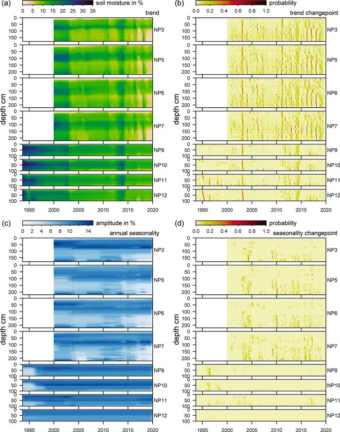
3520                                                                                 M. Merk et al.: Deep desiccation of soils

ter recharge was recorded (Kolusu et al., 2019). Similarly,       as well as determination of incoming water at the land sur-
Solander et al. (2020) found evidence for both increase (east-    face due to precipitation and non-rainfall events like dew or
ern Africa) and decrease (northern Amazon basin, the mar-         fog (Groh et al., 2018). Furthermore, they are used for deter-
itime regions of southeastern Asia, Indonesia, New Guinea)        mination of preferential flow (Schoen et al., 1999; Allaire
in soil moisture storage depending on location. An increase       et al., 2009), particle transport (Prédélus et al., 2015) and
in catchment evapotranspiration was observed during the           contaminant transport in the vadose zone Goss et al. (2010).
past decades (Duethmann and Blöschl, 2018). As groundwa-             There are about 2500 lysimeters installed at around 200
ter recharge is dependent on the availability of excess soil      sites across Europe, around half of them in Germany (Soł-
moisture, aquifers respond to climatic periodicities (Liesch      tysiak and Rakoczy, 2019). In the present study, we analyze
and Wunsch, 2019).                                                long-term soil moisture time series from two large inclined
   Traditionally, soil moisture was determined by taking rep-     lysimeters located in southern Germany. Data from the mon-
resentative soil samples for gravimetric determination, fol-      itoring of this test site have previously been evaluated and
lowing oven drying. The main disadvantage of this method,         published concerning the proper function of the landfill cover
despite being very precise, is its destruction of the sam-        (Zischak, 1997; Gerlach, 2007) and with regard to flow pro-
pling location and the sample itself. Achievement of long-        cesses on steep hillslopes (Augenstein et al., 2015) using
term data sets is challenging using this method. Non-             only much shorter parts of the time series available.
destructive measurement methods include cosmic ray neu-              However, a time-series analysis of all available soil mois-
trons (Rivera Villarreyes et al., 2011; K˛edzior and Zawadzki,    ture measurements from this test site to gain insight into
2016), installation of TDR sensors (Li et al., 2019), thermal     long-term soil moisture variations has not been done previ-
infrared sensors (Yang et al., 2015), resistivity measurements    ously and is the main focus of this study. The inclusion of
like the OhmMapper (Walker and Houser, 2002), capacitance         previously unpublished data from the more recent soil mois-
measurements or neutron probes (Hodnett, 1986; Evett and          ture measurements allows for a more comprehensive analy-
Steiner, 1995). A comparison and a discussion of several          sis of the time series. Using the available data from this test
sensor systems using different measurement principles are         site, it is possible to identify past events that led to signifi-
given in Jackisch et al. (2020), highlighting also the need for   cant changes in the long-term dynamics of soil moisture. The
thorough calibration before the use of such systems. During       main research questions are the following.
this study two calibrated neutron probes were used. Numer-
ical approaches include modeling of depth-dependent soil              – How did the measured soil moisture levels change over
moisture based on surface measurements (Qin et al., 2018)               the past decades?
or modeling of soil moisture for specific locations based on          – Can these changes be described by simple linear mod-
available weather data (Menzel, 1999). Another modeling                 els, or does it require more sophisticated modeling ap-
approach of soil moisture is based on remote-sensing data.              proaches?
This has been done on catchment scale (e.g., Pellenq et al.,
2003; Penna et al., 2009), regional scales (e.g., Mahmood             – Can exceptional hydro-meteorological events that had
et al., 2012; Otkin et al., 2016; Long et al., 2019) and the            a lasting impact on soil moisture levels be identified as
global scale (e.g., Dorigo et al., 2017; Albergel et al., 2020)         tipping points by statistical methods?
with various calculation grid sizes and temporal resolutions.
Analysis of inherent parameter uncertainty in modeled soil            – Are there seasonal differences? During which time of
moisture and implications for current discussions about soil            the year did the greatest change in soil moisture level
moisture dynamics should be considered (Samaniego et al.,               occur?
2012) as well as upscaling of measurements to different tem-
                                                                      – Which part of the soil is affected the most?
poral and spatial scales (Mälicke et al., 2020).
   Lysimeters are also suitable for gaining in-depth knowl-
edge about water balance and water movements in soil,             2    Study site
which is the main reason the lysimeter in this study is op-
erated. It provides a direct measurement of percolation rates     The study site is located in southern Germany (8.337 ◦ N,
through the soil, which makes it suitable for monitoring and      49.019 ◦ E) near the city of Karlsruhe (Fig. 2). The climate in
demonstration of equivalency of the earthen landfill cover        the region is classified as warm temperate, fully humid with
(Abichou et al., 2006). Application of lysimeters, however, is    warm summers or as Cfb according to the Köppen–Geiger
not restricted to monitoring of legally acceptable percolation    classification scheme (Beck et al., 2018; Kottek et al., 2006).
rates but also allows for studies into water and solute trans-    Mean annual precipitation is 760 mm (1990–2007, DWD
port in the vadose zone that would not be possible by other       station 2522, Karlsruhe). Annual precipitation and temper-
means (Singh et al., 2018). Their usage allows for precise de-    atures are shown in Fig. 1. Exceptionally dry years within
termination of evapotranspiration (ET) if soil water storage is   the observation period between 1994 and 2019 are 2003
accounted for to well below the root zone (Evett et al., 2012)    with 566.3 mm and 2018 with 566.7 mm of precipitation.

Hydrol. Earth Syst. Sci., 25, 3519–3538, 2021                                       https://doi.org/10.5194/hess-25-3519-2021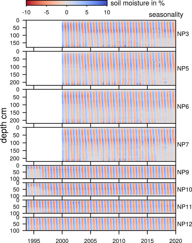
M. Merk et al.: Deep desiccation of soils                                                                                     3521

                                                                   (Berger, 2015). For the year 2002, the porosity of the RL is
                                                                   0.4 (–), usable field capacity 0.25 (–) and the wilting point at
                                                                   0.14 (–). The permeability was estimated as kf = 1.0 × 10⁻⁶
                                                                   (ms−1 ). Formation of preferential flow paths in the lysime-
                                                                   ter led to changes in hydraulic properties over time (Gerlach,
                                                                   2007).
                                                                      Both fields are covered by grass and weeds, depending on
                                                                   the current season. The growth of deeply rooted plants that
                                                                   would damage the sealing system is prevented, and the grass
                                                                   is cut regularly on the complete landfill cover including both
                                                                   lysimeters. In recent years, sheep have been used to limit the
                                                                   growth of vegetation in a more natural way. Further records
                                                                   on the vegetation cover and plant maintenance are not avail-
Figure 1. Precipitation and temperature at stations 2522
                                                                   able.
(January 1994–October 2008) and 4177 (November 2008–
December 2019) (DWD Climate Data Center (CDC), 2020).

                                                                   3     Material and methods

The highest annual precipitation was recorded in 2002 with         3.1    Soil moisture and discharge measurements
981.6 mm, followed by 2013 with 972.4 mm of precipitation.
Mean annual temperature was highest in 2018 (12.33 ◦ C) and        Soil moisture measurements were carried out using two dif-
lowest in 1995 (9.69 ◦ C).                                         ferent neutron probes. A modified Wallingford IH2 neutron
   Two large inclined lysimeters are embedded in the mu-           probe was used until 23 August 2012. From 30 Novem-
nicipal landfill site Karlsruhe-West for mandatory monitor-        ber 2012 onward, a modified Troxler 4300 depth moisture
ing purposes. Cross sections of both lysimters are shown in        gauge was used. Both models used an Am/Be source with
Fig. 3. The first lysimeter (Field 1) was built in 1993 and        activities of 1.85 GBq and 370 MBq, respectively (Augen-
started operation at the end of that year. With a width of 10 m    stein et al., 2015). They were modified to fit into the installed
and a length of 40 m, it has a size of 400 m2 . The mean in-       measurement tubes. Selected measurement points are shown
clination angle is 23.5◦ (43.5 %) with a southern exposition.      in Fig. 2. Neutron probe measurement points (NPs) are con-
The recultivation layer (RL) in this field has a thickness of      structed from steel tubes (∅ 40.5 mm) installed vertically in
100 cm; it is underlain by a drainage layer (DL) with a thick-     the soil column. At neutron probe measurement points 9
ness of 15 cm followed by a mineral clay liner (MCL) and           through 12 (NP9, NP10, NP11, NP12) located in lysimeter
capillary barrier.                                                 Field 1, measurements were carried out on a weekly basis
   The second lysimeter (Field 2, pictured in Fig. 4) was built    until Field 2 was constructed (December 2000). After con-
in 2000, with the first measurements being taken in Decem-         struction of Field 2, measurements were taken monthly in
ber of that year. It consists of two separate fields with a size   Field 1. At the same time, weekly measurements in Field 2
of 10 m by 20 m each, resulting in a total size of 400 m2 . The    at neutron probe measurement points NP3, NP5, NP6, and
mean inclination angle is 23.5◦ (43.5 %) with southern ex-         NP7 started. Measurements were taken in depth increments
position. Results from Field 1 showed that a thicker RL is         of 10 cm until the bottom of the lysimeter was reached (fi-
necessary in order to protect the MCL from drying out. This        nal depth Field 1: between 2.1 and 2.3 m; final depth Field 2:
insight was considered during the construction of Field 2.         between 2.8 and 3.4 m). No measurements were taken at the
The RL in Field 2A has a thickness of 200 cm, and in Field         remaining four points in Field 2. During the period of Jan-
2B it has a thickness of 215 cm. It is underlain by a DL with      uary to June 2014, no measurements were taken at either of
a thickness of 15 cm followed by a mineral clay liner and          the two fields due to ongoing construction of new accessibil-
capillary barrier. Depth across the inclined field varies. Ad-     ity stairs for Field 2.
ditionally, the mineral clay liner is not present in the lower        Discharge from the drainage pipes (Fig. 3) is collected in
half of Field 2B, reducing the final depth of the lysimeter by     cylindrical tubes equipped with magnetic valves at the bot-
50 cm, affecting measurements taken at NP5 and NP6 below           tom. A data logger connected to pressure sensors in each
the RL. The RL was constructed by adding layers of soil on         tube records water levels at regular intervals. Additional data
top of the compacted surface of the previous layer. Use of dif-    points are recorded when the changes in water levels are
ferent materials in the soil layers cannot be ruled out. Further   large. Once the tube is full, the valve at the bottom opens
details on the construction of both fields are given in Augen-     and closes automatically to empty the tube.
stein et al. (2015). The soil properties of the RL relevant to        From changes in the recorded water levels, discharge was
this study have been modeled by Gerlach (2007) using HELP          calculated. The area of the lysimeter field was used to cal-

https://doi.org/10.5194/hess-25-3519-2021                                       Hydrol. Earth Syst. Sci., 25, 3519–3538, 2021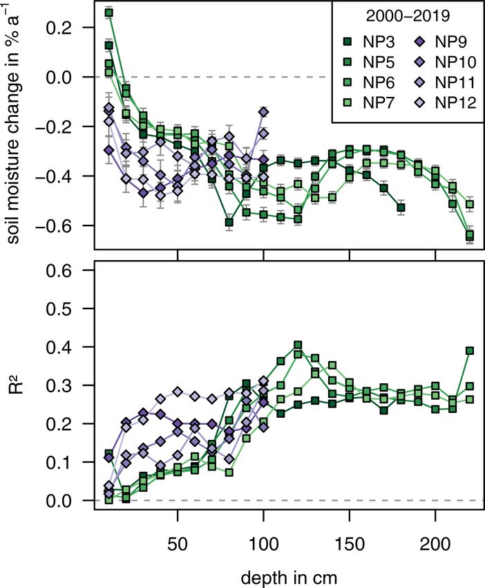
3522                                                                                        M. Merk et al.: Deep desiccation of soils

Figure 2. Location of the study site on a municipal landfill site in Karlsruhe, Germany, and locations of the weather stations used in this
study. Lysimeter 2 consists of two separate fields (Field 2A, Field 2B).

                                                                        culate monthly aggregated discharge per area (mm) from the
                                                                        amount of water that was collected (L).

                                                                        3.2   Additional data

                                                                        Additional data used for this study include daily precipitation
                                                                        and modeled values of usable field capacity (uFC). Daily pre-
                                                                        cipitation data at a station near Karlsruhe are published by the
                                                                        German weather service (DWD) (DWD Climate Data Cen-
                                                                        ter (CDC), 2020). Data for this station (station ID: 2522) are
                                                                        available for the time range until October 2008. Another sta-
                                                                        tion, still in operation by the DWD, is located in Rheinstetten
                                                                        (station ID: 4177), approximately 5 km south of the test site,
                                                                        providing data from November 2008 onward. Locations of
Figure 3. Cross sections of lysimeter Field 1 and Field 2 with the      both weather stations are shown in Fig. 2.
different layers and moisture measurement points.                          The DWD also publishes derived model results for usable
                                                                        field capacity (uFC) (DWD Climate Data Center, 2020) that
                                                                        can be used for comparison of measured soil moisture time
                                                                        series. They are provided for two different soil types and as
                                                                        depth-resolved values for the top 60 cm of the soil column.
                                                                        They are computed by the agrometeorological model AM-
                                                                        BAV. For this study the depth-resolved values for soil mois-
                                                                        ture under grass with sandy loam (wilting point 0.13 (–),
                                                                        field capacity 0.37 (–)) were used. Additionally, soil mois-
                                                                        ture under grass and loamy sand (wilting point of 0.03 (–),
                                                                        field capacity 0.17 (–)) up to 60 cm depth was used. A de-
                                                                        fined constant water content is used as the boundary con-
                                                                        dition at the bottom of the model. Further model input pa-
                                                                        rameters are hourly values of temperature, dew point, wind
Figure 4. Lysimeter Field 2 (visible in the upper part of the image     speed, precipitation, global radiation and reflected long-wave
between vertical beams).                                                radiation. Data were used from five stations (Table 1: 4177,
                                                                        377, 3925, 5275, 257, Fig. 2) and cover a time range from
                                                                        1 January 1991 until 31 December 2019. Values at station
                                                                        3925 are available from 2005 onwards. Measured soil mois-

Hydrol. Earth Syst. Sci., 25, 3519–3538, 2021                                             https://doi.org/10.5194/hess-25-3519-2021
M. Merk et al.: Deep desiccation of soils                                                                                    3523

ture data are not directly comparable to uFC because of a
different scale being used. The uFC of 100 % is defined as
the soil moisture content that cannot be drained by gravity.
Nonetheless, both measured soil moisture and usable field
capacity have similar temporal distribution patterns.

3.3   Theory and calculations

Volumetric water content (θ ) and uFC are expressed as %.
Data analysis and visualization were done in the R system
for statistical computing R Core Team (2020).
   Time series were transformed into a radial coordinate sys-
tem to highlight the asymmetry of the seasonal cycle between
gradual drying and fast re-wetting of the soil. New x and y
coordinates for each measurement were calculated according       Figure 5. Example of the calculation of monthly linear regressions
to Eqs. (1) and (2).                                             for April and September at NP 3 and at a depth of 170 cm.


                dyear                                            each measurement point, depth and month. An example of
x = cos 2 · π ·         ·θ                                 (1)
                 d/a                                             these calculations is shown in Fig. 5 for the months of April
                                                                 and September at NP3 and at a depth of 170 cm.

                dyear
y = sin 2 · π ·         ·θ                                 (2)      Measurements at Field 1 were taken weekly at the start
                d/a
                                                                 of the time series, but the interval changed to monthly mea-
   In these two equations, x and y are the new coordinates       surements later. Therefore, use of all values for regression
in a radially transformed coordinate system, and θ is the vol-   would lead to an overemphasis of the early part of the time
umetric water content in percentage. dyear is the day of the     series, due to the higher number of samples during that time
year. It is divided by the length of the respective year (d/a)   span. To avoid this bias and overemphasis, monthly averages
in order for 2π to equal 1 year.                                 were used. The regressions yielded individual values for the
   Mean soil moisture of the recultivation layer in Field 2      change in soil moisture by month and depth. Additionally,
was calculated as the average of NP3 at depths between 10        further information about the regressions was extracted from
and 180 cm and at NP5, NP6 and NP7 at depths between 10          the results. These include standard deviations and p values
and 220 cm.                                                      for the slopes. The analysis was done with the time series of
   For each individual depth, a linear regression was cal-       uFC in a similar fashion.
culated using all measurements for the years 2000 to 2019           Time-series analyses are sensitive to the selection of a suit-
(see Sect. 3.1). Calculations were done using the lm() func-     able model. To overcome the paradigm of the single-best
tion in the R system for statistical computing (R Core Team,     model approach in time-series decomposition, Zhao et al.
2020). As linear regression can be dependent on the selected     (2019b) implemented a Bayesian model averaging scheme
start and end times, additional regressions were calculated      to approximate complex relationships by the use of Markov
over the complete available time span, based on time series      chain Monte Carlo stochastic sampling. The model space is
cut off before 2004 and between 2004 and 2016. The re-           explored by randomly traversing through combinations of
sulting slopes of these regression lines represent the mean      coefficients. The number and location of individual change
change in soil moisture in %d−1 . A conversion into %a−1         points in seasonality and trend are randomly sampled and all
was calculated by using the average length of 365.2425           candidate models averaged based on how probable each of
d a−1 , according to the Gregorian calendar.                     them is. Results of the model not only include best estimates
   To overcome the limitations of linear regressions when        for model parameters (e.g., location of change points), but
used on data with large seasonal variation compared to a         also their probability distributions. Bayesian change-point
small overall trend, another set of linear trends was calcu-     detection and time-series decomposition were done using the
lated based on monthly averages. The monthly values were         beast() function from the Rbeast package (Zhao et al.,
calculated as averages based on the measured values within       2019a). This divides the time series into seasonal and trend
each month and depth. No weights were assigned to individ-       components, along with change points in both. The period
ual measurements. The time series for all depths were each       was set to 12 for monthly time-series decomposition. The
subdivided into 12 time series, 1 for each month. For ex-        same monthly averaged time series were used as with the
ample, application of this subdivision to the time series at     previous monthly linear regressions.
a depth of 170 cm at NP3 results in 12 time series (Fig. 5).
Linear regressions were then calculated separately, based on
all mean values for each month, giving the average slope for

https://doi.org/10.5194/hess-25-3519-2021                                     Hydrol. Earth Syst. Sci., 25, 3519–3538, 2021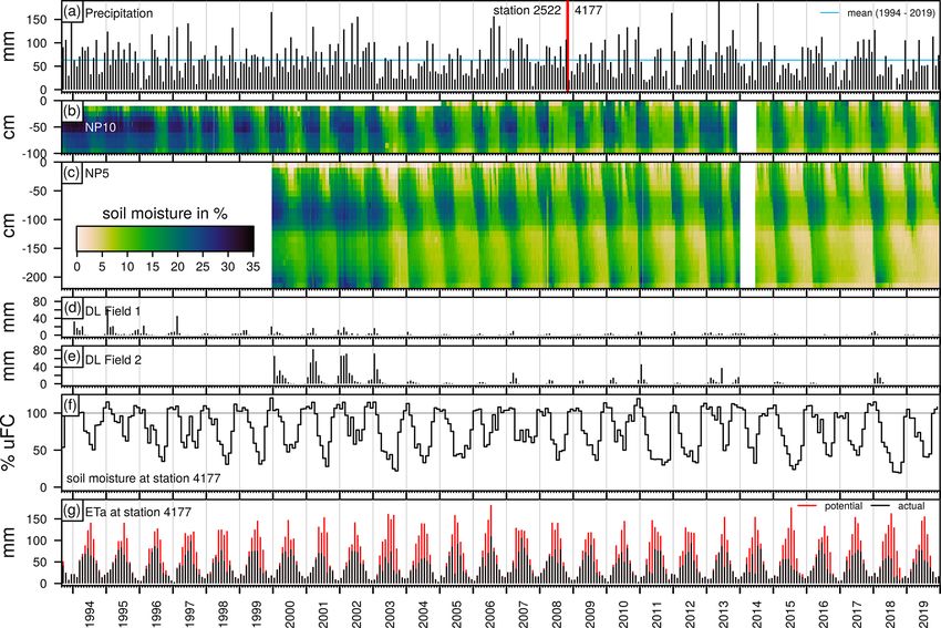
3524                                                                                            M. Merk et al.: Deep desiccation of soils

Table 1. Locations of weather stations and distances to the test site.

                         Station name                 Station ID    Elevation       Latitude    Longitude   Distance
                         Karlsruhe                         2522     112 m a.s.l.    49.0382◦    8.3641◦     2.9 km
                         Rheinstetten                      4177     116 m a.s.l.    48.9726◦    8.3301◦     5.2 km
                         Bad Bergzabern                     377     210 m a.s.l.    49.1070◦    7.9967◦     26.7 km
                         Pforzheim-Ispringen               3925     333 m a.s.l.    48.9329◦    8.6973◦     28.1 km
                         Waghäusel-Kirrlach                5275     105 m a.s.l.    49.2445◦    8.5374◦     29.0 km
                         Baden-Baden-Geroldsau              257     240 m a.s.l.    48.7270◦    8.2457◦     33.2 km

4   Results                                                                ET, once again drying out the lower soil and no re-wetting
                                                                           occurring in the winter months.
                                                                              Soil moisture in Field 1 is higher at the upper slope (NP9)
The study represents a very specific case, and the interpre-               compared to the lower slope (NP12), especially at the start
tation of results is limited to these specific conditions at the           of the measurement series (Fig. A1). As with Field 2, soil
landfill.                                                                  moisture levels are lower after 2003. Because the RL is not
   Measured soil moisture values in the RL at NP5 and NP10                 as thick in Field 1 (100 cm) compared to Field 2 (∼ 215 cm),
are presented in Fig. 6 at the corresponding position on the               re-wetting in the lower soil at depths below 100 cm is not
respective soil moisture profiles and before monthly averages              observable. However, in years with missing re-wetting (e.g.,
were calculated. There is a gap in measurements during the                 2017, 2019) of lower soil in Field 2, a similar gap can be
first half of 2014. Field 2 was built in 1999, and no data                 observed in Field 1 below the MCL (∼ 200 cm). In data
are available prior to the year 2000. In total, over 140 000               from Field 2, depth dependence of soil moisture is clearly
individual soil moisture measurements are shown. Due to                    evident. Higher soil moisture at depths of around 100 cm
grain size and soil properties, the mineral clay liner has a               sharply decreases over the next 20 cm, and downward prop-
higher moisture content (> 25 %). It is overlain by the gravel             agation of the moisture front is also delayed. This effect is
drainage layer, which has a very low moisture content. For                 caused by differences in soil compaction during construc-
evaluation, only soil moisture content of the RL is used in                tion of the lysimeter and possibly the use of different soil
this study (n = 91 198), because it is thought to be the layer             materials. The volume of the lysimeter was filled in several
in the lysimeter that reflects best the processes and moisture             layers and soil consolidated in between each. Porosity and
dynamics found in natural soils.                                           hydraulic conductivity is therefore not uniformly distributed
   From this figure, a seasonal pattern is clearly visible. Soil           over the complete depth of the lysimeter. The greatest differ-
moisture increases relatively quickly in late fall or winter, es-          ences are found at the interfaces of two consecutive stages
pecially in the upper parts of the soil. After reaching a critical         of construction between the strongly consolidated top of the
soil moisture level, discharge from these layers starts more or            underlying layer and the less densely packed bottom of the
less instantaneously and is measured as discharge from the                 overlying layer. The consistent and very distinct break of soil
DL. This wetting period is followed by a more gradual dry-                 moisture over the entire measurement period suggests that
ing period, starting in late spring and lasting until the consec-          there is a distinct change in porosity and hydraulic conductiv-
utive wetting period. The years before 2003 appear to have                 ity between these two layers. Settling down of the soil cover
higher soil moisture content and shorter drying seasons, es-               in the years after construction may additionally change soil
pecially at, but not restricted to, Field 2. This can be seen              properties over time.
for example at NP5 in Field 2, where blue colors, indicat-                    Values of modeled uFC are also shown in Fig. 6 for DWD
ing soil moisture of over 30 %, alternate with green colors                station 4177 under grass and loamy sand.
(15 %) before 2003. After 2003, green colors alternate with
yellow colors, indicating soil moisture below 10 %. In recent              4.1     Drainage data and discharge behavior
years, the re-wetting of the soil during the winter month re-
peatedly did not reach the lower parts of the soil, especially             Discharge from the drainage layer is shown in Fig. 6d and e.
in Field 2. For example, at NP5 at depths between 100 cm                   It follows a seasonal pattern with the highest discharges be-
and 200 cm, yellow colors indicate soil moisture levels be-                ing recorded at the beginning of the year, usually around the
low 5 % for the complete years 2017 and 2019. Measured                     months of January or February. During the summer months,
discharge during these years was significantly lower com-                  discharge is lowest and can be completely absent, especially
pared to the prior years. Despite above-average precipitation              in recent years. The onset of discharge is usually more or less
during the second half of 2017, re-wetting was only observed               instantaneous, with the highest rates of discharge measured
much later in early 2018. Precipitation in 2018 was well be-               around the time discharge starts. Augenstein et al. (2015) an-
low average and paired with a large atmospheric demand for                 alyzed the discharge behavior as a function of the soil mois-

Hydrol. Earth Syst. Sci., 25, 3519–3538, 2021                                                  https://doi.org/10.5194/hess-25-3519-2021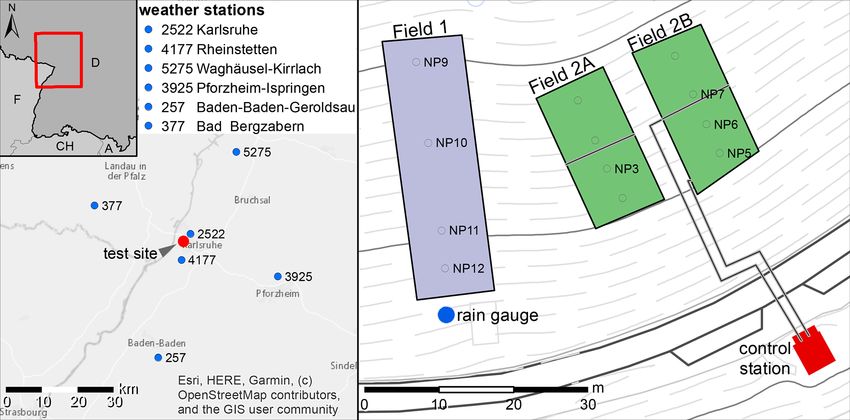
M. Merk et al.: Deep desiccation of soils                                                                                            3525

Figure 6. (a) Monthly precipitation at stations 2522 (January 1994–October 2008) and 4177 (November 2008–December 2019) (DWD
Climate Data Center (CDC), 2020). Blue line represents mean monthly precipitation during 1994 to 2019. (b, c) Time series of selected soil
moisture measurements (NP5 and NP10, respectively) at the test site near Karlsruhe, Germany. (d, e) Monthly discharge of the drainage layer
(DL) at both lysimeters. (f) Simulated monthly averages of usable field capacity (loamy sand). (g) Monthly values of simulated potential
evapotranspiration (red) and simulated actual evapotranspiration (black) (DWD Climate Data Center, 2020) at station 4177. Measurements
on Field 2 are available from 2000 onward. No measurements were taken during the first half of the year 2014.

ture. It usually takes the soil moisture front several weeks to         2003. This reduction in drainage coincides with a reduction
percolate through the soil column and eventually drain. Indi-           in soil moisture in both fields. In recent years when the soil
vidual precipitation events during the drier summer months              moisture front did not reach the lower parts of the soil col-
do not lead to an immediate onset of discharge from the                 umn, there was no discharge from the DL.
lysimeter. However, precipitation events during the discharge
period may rapidly increase the amount of discharge. The                4.2   Asymmetry of drying and re-wetting
soil moisture near the bottom of the soil column at the ini-
tial onset of discharge is usually lower than the soil moisture
when the discharge stops.                                               To highlight the asymmetry of the seasonal cycle between
   Water flow is also influenced by the slope. The soil mois-           gradual drying and fast re-wetting of the soil, two exemplary
ture front on the upper slope usually takes longer to reach             time series are shown in a polar coordinate system (Fig. 7).
equivalent depth on the lower slope, meaning the lower slope            For comparison, the soil moisture time series of NP3 at a
usually gets wet more quickly, indicating a strong lateral              depth of 170 cm and a mean time series from all sampling
component of sub-surface water flow (Augenstein et al.,                 points at Field 2 are shown. The overall trend of both time
2015).                                                                  series is quite similar; however, the asymmetry is much more
   Initially, after construction of the lysimeter, discharge was        pronounced in the time series of NP3 at 170 cm. The mean
noticeably higher in comparison to later years. This is more            of all soil moisture time series in Field 2 was calculated over
pronounced in Field 2 (Fig. 6e). A significant reduction in             the complete depth of the recultivation layer (RL). Due to
annual discharge from the DL can be seen around the year                the lag in the downward propagation of soil moisture in the
                                                                        profile, the asymmetry of the seasonal cycle is evened out by

https://doi.org/10.5194/hess-25-3519-2021                                             Hydrol. Earth Syst. Sci., 25, 3519–3538, 2021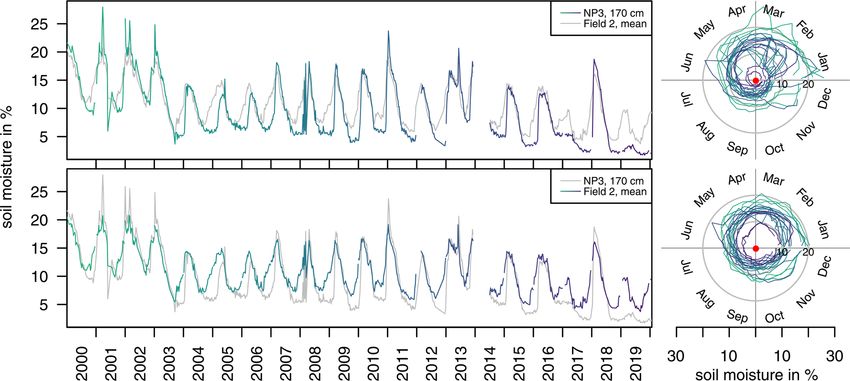
3526                                                                                   M. Merk et al.: Deep desiccation of soils

calculation of the mean soil moisture over multiple depths          nificant decrease in soil moisture. The moisture change in
and measurement points.                                             the top 60 cm of the soil does show an increase during sum-
   In the two time series shown in polar coordinates, the           mer, but this increase is not statistically significant. The lack
graph based on mean values describes a circle for each year         of statistical significance might be due to the shorter length
of observation. In the time series of NP3 at 170 cm, on the         of the time series at Field 2 compared to Field 1. As pre-
other hand, the graph describes spirals resembling nautiluses       viously mentioned, overall soil moisture levels were higher
for each year of observation. The decreasing radius over            before 2003. Inclusion of additional data before this point, as
time, apparent from both time series, indicates a decrease in       is the case with Field 1, would push the resulting decrease in
soil moisture. White areas between lines indicate large and         soil moisture towards higher absolute values. From depths of
sudden changes in soil moisture levels during especially dry        around 70 to 130 cm (70 to 90 cm at NP3), decrease in soil
years. The opening of the nautilus corresponds to a rapid in-       moisture has a semiannual distribution. The highest reduc-
crease in soil moisture during winter. Depending on precip-         tions in soil moisture occurred during November and Decem-
itation conditions, this increase may occur at the end of the       ber as well as during April and May. Below this, decrease in
year or the beginning of the consecutive year.                      soil moisture is generally lower and does show a weak annual
                                                                    cycle with the highest values in December and January and
4.3    Overall linear regressions                                   minima during June and July. The highest values are shown
                                                                    in the lowermost 30 cm of the RL directly above the DL be-
In Fig. 8, results of individual linear regressions of soil mois-   tween January and May.
ture measurements are shown for each depth and measure-                In Field 1, a decrease in soil moisture can be observed at all
ment point. Over the period between 2000 and 2019, soil             depths. The semiannual distribution of soil moisture change
moisture decreases by 0.34 ± 0.14 %a−1 within the RL. The           is similar to that of Field 2. It is most pronounced during
observed decrease is lowest in the first 20 cm of the soil col-     spring and fall and less pronounced during winter and sum-
umn at both lysimeter fields. At a depth of 10 cm there is even     mer.
a small increase observable in Field 2.                                The winter months are usually times of the largest ground-
   Overall, the decrease in soil moisture is most pronounced        water recharge and the highest soil moisture in the lower soil.
at depths of 20 to 40 cm in Field 1 (NP9, NP10). Due to             In recent years, however, less water percolated through the
the thicker RL compared to Field 1, the highest absolute            upper parts of the soil at both lysimeter fields, affecting es-
decrease is found at a greater depth of around 100 cm in            pecially the soil moisture levels in the lower soil. This dry-
Field 2. Below 130 cm in Field 2, the absolute rate of soil         ing effect is amplified by the DL. It drains excess water and
moisture change is slightly lower. Seasonal variations of soil      inhibits capillary rise. This means the depth of evapotranspi-
moisture patterns larger than the overall trend lead to a rela-     ration in the lysimeter is greater than 2 m and includes the
tively low coefficient of determination (0.20 ± 0.10). How-         complete RL.
ever, with the exception of two points (NP5 20 cm, NP7                 Results of linear regressions based on monthly averages of
10 cm), all slopes of calculated regression lines are signif-       uFC are shown in Fig. 10. Most values indicate a decrease in
icant (p < 0.05, n = 122). Coefficients of determination are        soil moisture, but at the same time, most linear regressions
lowest at the top and increase until a depth of around 100 cm.      are not statistically significant (p > 0.05). However, results
Precipitation events lead to short-term variations in soil mois-    for station 5275 indicate a clear and significant decrease in
ture. These variations are larger at the surface. Downward          soil moisture during most of the year. The decrease in the
movement of the water in the soil column is being damp-             lower soil layers appears to happen later in the year. Com-
ened with depth. At some depths, soil moisture patterns are         pared to Fig. 9, the semiannual pattern is not as visible, but
more persistent. This might be due to different materials be-       some months (August at stations 4177, 377, 5275, and 257)
ing used or differences in compaction during construction of        do show lower annual changes or even an increase in uFC
the lysimeters and landfill cover. Differing soil properties like   (January at station 3925).
porosity, hydraulic conductivity and capillary forces deter-           Compared to the largest decrease in measured soil mois-
mine the water retention capacity of the soil.                      ture at the beginning of the vegetation period in April and at
                                                                    the end of the vegetation period in November, the decline of
4.4    Monthly linear regressions                                   uFC at the end of the vegetation period appears to happen
                                                                    much earlier (3925, 5275).
The results of linear regressions based on the monthly av-
erages are shown in Fig. 9. Resulting slopes with p > 0.05          4.5   Time-series decomposition
(i.e., soil moisture change is not significant) are indicated by
a marker.                                                           During modeling with Rbeast, the time series are decom-
   A statistically significant increase in soil moisture can be     posed into a trend component and a seasonal component,
observed in the top 10 cm of Field 2 (NP3, NP5, NP6, NP7)           along with change points in both seasonality and trend. In-
during the winter months only. Most other values show a sig-        dividual calculations are done for each depth increment at

Hydrol. Earth Syst. Sci., 25, 3519–3538, 2021                                        https://doi.org/10.5194/hess-25-3519-2021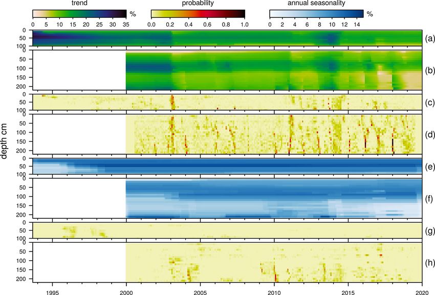
M. Merk et al.: Deep desiccation of soils                                                                                             3527

Figure 7. Time series of soil moisture at NP3 at 170 cm and mean soil moisture of Field 2 as well as the same data in a polar coordinate
system to highlight seasonal asymmetry of gradual drying and fast re-wetting as well as the overall trend of declining soil moisture. Colors
indicate the year of the measurement. For context, gray lines showing mean soil moisture of Field 2 and soil moisture at NP3 at 170 cm,
respectively, were added.

                                                                        level after a significant decrease in soil moisture levels be-
                                                                        tween February and December. Changes in seasonality were
                                                                        detected in 2004 and 2006/2007. In between these, the am-
                                                                        plitude of the seasonal variations was lower.
                                                                           In Fig. 12 the main results of this model are shown for
                                                                        a measurement point in Field 1 (NP5) and Field 2 (NP10).
                                                                        This kind of decomposition allows for easier visual analy-
                                                                        sis of the underlying trend component (Fig. 12). Probabili-
                                                                        ties of change-point occurrence indicate times of significant
                                                                        changes in trend and seasonality. Overall, higher soil mois-
                                                                        ture contents are apparent before 2003 and during a shorter
                                                                        time period in 2013/2014. In the past few years, soil moisture
                                                                        is noticeably lower, especially at depths below 100 cm.
                                                                           The decomposed time series of NP10 in Field 1 (NP9–
                                                                        NP12 in Fig. A5) reveal higher initial soil moisture contents,
                                                                        followed by a gradual decrease over time. The decrease is
                                                                        most pronounced at the beginning of the measurement se-
                                                                        ries, until around 1998 a more or less stable level of soil
                                                                        moisture is reached. The amplitude of seasonality at the top
                                                                        of the slope (NP9 and NP10) during this time of high ini-
                                                                        tial soil moisture is lower. This is probably due to the max-
Figure 8. Results of individual linear regressions for soil moisture    imum saturation of the soil being reached, leading to an in-
measurements in hthe recultivation
                        i          layer, expressed as change in soil   crease in discharge from the soil instead of further increase
moisture content %a−1 .                                                 in soil moisture content and storage. In 2003, a change point
                                                                        in trend is visible. Modeling resulted in high probabilities for
                                                                        this change point. In the following years, the soil moisture is
                                                                        at a lower level. Apart from the elevated soil moisture before
all measurement points. An example of NP3 at a depth of
                                                                        2003, higher soil moisture is also evident in 2013. The dis-
170 cm is given in Fig. 11. The trend component shows a
                                                                        tribution of probabilities for a change point in trend does not
positive slope before 2003. A change point in trend with a
                                                                        show a clear cut during this event. Probabilities are elevated
probability of 68 % was discovered in February of 2003. Af-
                                                                        over a wider range of time. The amplitude of soil moisture
ter another change point with a lower probability in Decem-
ber 2003 (17 %), the soil moisture trend stabilized at a lower

https://doi.org/10.5194/hess-25-3519-2021                                             Hydrol. Earth Syst. Sci., 25, 3519–3538, 2021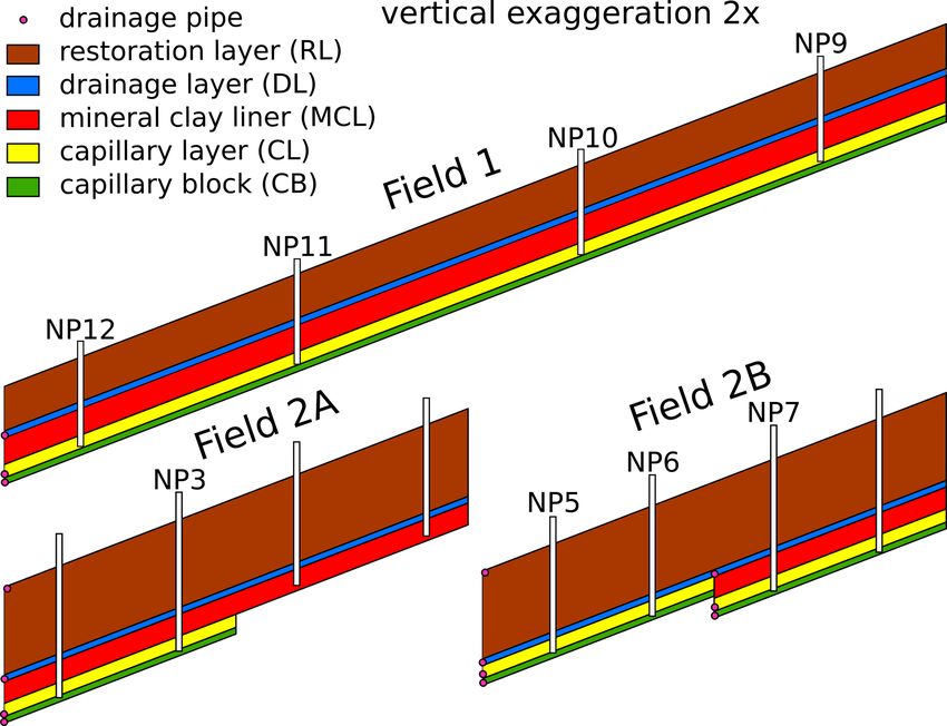
3528                                                                                       M. Merk et al.: Deep desiccation of soils

Figure 9. Resultsh of individual
                         i       linear regressions for soil moisture measurements in the recultivation layer, expressed as change in soil
moisture content %a−1 calculated over the complete time series for each month based on monthly averages. Upper graphs: Field 2, lower
graphs: Field 1. Values for p > 0.05 are indicated by a marker.

seasonality is more or less stable for the remainder of the            time, reduction of soil moisture to a low level not observed
time series and does not show high probabilities.                      previously occurs, mainly in the lower half of the RL. Be-
   Measurements at Field 2 (NP 3, NP5, NP6, NP7) also                  cause of a thinner RL, this effect cannot be observed in Field
show higher initial soil moisture contents. As previously              1. In recent years from 2015 onward, amplitude of seasonal
mentioned, depth dependence of soil moisture due to lysime-            variation in the lower half of the RL is greatly reduced, be-
ter construction is also visible in the deconstructed time se-         cause dry soil without the reoccurring annual re-wetting does
ries. No apparent trend is observable until the year 2003. A           not show significant seasonality.
change point in trend and the corresponding probabilities is              Interruption of capillary rise due to lysimeter construction
then visible around the same time as in Field 1. In the follow-        inhibits re-wetting of the lower soil from groundwater. Thus,
ing year (2004) a change point in seasonality with elevated            results of this study might not be applicable to soils with a
probabilities in the lower half of the RL at Field 2 occurred.         shallow depth to the groundwater surface or modeled val-
Slightly elevated probabilities for this change point were al-         ues of usable field capacity. Boundary conditions are differ-
ready calculated for the year 2003 itself. In general, ampli-          ent for the modeled usable field capacities analyzed in this
tudes of seasonal variations are higher towards the top of the         study. They are calculated from weather data and standard-
RL. After the 2003 change point, higher amplitudes of sea-             ized soil properties. An additional source of soil moisture is
sonal variation are found lower in the RL than before (NP3,            provided by capillary rise due to a constant moisture bound-
NP5, NP6). At NP7 (Fig. A5), the amplitude of seasonal vari-           ary condition at the bottom of the model. The fact that some
ations at a depth of 80 cm increased after this point, but am-         stations did show the same patterns as measured soil mois-
plitudes in the soil below are significantly lower.                    ture, while other stations with the same soil properties did
   Another visible change point in trend with elevated proba-          not, could mean that there are feedback mechanisms between
bilities is visible at the end of 2011. This change point cannot       soil moisture and the input parameters of the uFC model. Fu-
be seen in Field 1. After 2015, change points with elevated            ture studies should concentrate on these interconnections be-
probabilities appear to occur almost every year. At the same           tween soil moisture, groundwater recharge and groundwater

Hydrol. Earth Syst. Sci., 25, 3519–3538, 2021                                            https://doi.org/10.5194/hess-25-3519-2021
M. Merk et al.: Deep desiccation of soils 3529
level to determine whether they amplify or dampen the tem-
poral dynamics of soil moisture.
5 Discussion
One possible explanation for the rapid change in soil mois-
ture levels could be a change in soil properties (water re-
tention, preferential flow paths, hydraulic conductivity, soil
structure, etc.) as a result of singular extreme events like the
exceptionally dry year 2003. Augenstein et al. (2015) found
that there are hysteresis effects during drying and re-wetting
of the soil at this site. Water bound in different states (e.g.,
adhesive water or water stored in the inter layers of clay
minerals) has different migration times. The proportion of
water bound in these different states therefore influences the
drainage behavior (Šimůnek et al., 2003). During the period
of increased soil moisture, water migrates into the inter layers
of the clay minerals (Schnetzer, 2017). This water cannot be
drained by gravity but still contributes to soil moisture. After
discharge from the lysimeter stops, desiccation of these clay
minerals may occur by evaporation into the soil air.
Another contribution factor might be changes in soil tem-
peratures (Vanderborght et al., 2017; Schneider et al., 2021).
These are usually highest around September and October.
Temperature has a great effect on viscosity of water and in-
Figure 10. Results of individual linear regressions for usable field fluences surface tension and contact angle, thus determining
capacity (uFC) for the top 60 cm (at stations 4177, 377, 3925,
h 5275,i how much water can be retained by capillary forces.
and 257), expressed as change in usable field capacity %a−1 Hydraulic conductivity in the vadose zone is dependent on
calculated over the complete time series for each month based on the moisture content. This feedback mechanism might am-
monthly averages. Statistically non-significant values (p > 0.05) plify or dampen the hysteresis, depending on the proportions
are indicated by a marker. of bound soil moisture in different states (available porewa-
ter, porewater in enclosed cavities). Furthermore, extreme
drying of the soil might lead to non-reversible desiccation
of clay minerals or formation of drying cracks as preferen-
tial flow paths, both leading to significant changes regarding
the overall hydraulic functioning of the whole system. How-
ever, though these likely phenomena may occur, changes in
soil water dynamics are also visible from the modeled uFC.
These are not based on physical measurements which are de-
pendent on time-constant soil properties, but rather use time-
constant properties of a model soil. The fact that these mod-
eled values also show changes in their temporal soil moisture
patterns gives ample evidence that the change points found
are not merely a function of soil properties but of the local
climate as well, which the modeled values are solely based
on.
Changes in measured soil moisture at around the year 2003
could also be the result of the establishment of a vegetation
cover after the construction of the lysimeter and over several
Figure 11. Results of time-series decomposition for NP3 at a depth consecutive years. The soil cover is important for preventing
of 170 cm. Change points and their respective probability distribu-
erosion and for lowering overall percolation by increasing
tions are shown also.
evapotranspiration. The system is designed with a vegetation
cover as an integral part of its proper functioning. However,
https://doi.org/10.5194/hess-25-3519-2021 Hydrol. Earth Syst. Sci., 25, 3519–3538, 20213530 M. Merk et al.: Deep desiccation of soils Figure 12. Results of modeling soil moisture at NP5 and NP10 with Rbeast. (a) Trend component of soil moisture time series at NP10 in Field 1. (b) Trend component of soil moisture time series at NP5 in Field 2. (c) Probability of a change point in the trend component at NP10 in Field 1. (d) Probability of a change point in the trend component at NP5 in Field 2. (e) Amplitude of annual seasonality derived from the seasonal component at NP10 in Field 1. (f) Amplitude of annual seasonality derived from the seasonal component at NP5 in Field 2. (g) Probability of a change point in the seasonality component at NP10 in Field 1. (h) Probability of a change point in the seasonality component at NP5 in Field 2. Field 1, which was constructed several years prior to Field 2, ambient humidity will then increase temperatures even fur- shows a similar change at the same time. ther, increasing the severity of a drought. A similar change is likewise visible in the modeled data, Robinson et al. (2016) found evidence for the existence of but a change in vegetation cover is not used as an input to the drought-induced alternative stable soil moisture states. They model. It is still possible that vegetation and evapotranspira- observed a step change that occurred at the beginning of tion both drive these changes in the model and the measured 2004 with an apparent transition to a new stable state in data, but then it has to be connected through the meteorologic which soil moisture levels never reached saturation again. parameters used in the model (e.g., longer vegetation peri- They found water retention characteristics to change due to ods). Ionita et al. (2020) found that prevailing large-scale at- a loss of organic material by increased organic matter min- mospheric circulation may impact atmospheric blocking over eralization under moderate drought conditions. According to the North Sea and central Europe and thus lead to extreme their findings, the bottom boundary behavior was modified weather being more persistent. If this is the case, the change from a seepage face behavior before 2004 to free drainage towards elevated temperatures would also lead to an exten- after. For arid regions, strong positive feedback between veg- sion of the vegetation period, thus increasing evaporation as etation and soil moisture has been described by D’Odorico a result of higher temperatures and plant transpiration as a et al. (2007). Small changes in environmental variables can result of the longer vegetation period. If evapotranspiration lead to rapid and irreversible shifts between two alternate sta- is limited by the amount of available water, the difference ble states (D’Odorico et al., 2007). between actual evapotranspiration and potential evapotran- spiration will increase. Less evaporative cooling and lower Hydrol. Earth Syst. Sci., 25, 3519–3538, 2021 https://doi.org/10.5194/hess-25-3519-2021
M. Merk et al.: Deep desiccation of soils                                                                    3531

6   Summary and conclusions

The aim of this study was to identify long-term variations of
soil moisture patterns and to identify the occurrence of par-
ticular events that led to tipping points in soil moisture levels.
To achieve this, we analyzed high-resolution soil moisture
measurements from a test site near Karlsruhe, Germany. The
data consist of depth-resolved, weekly soil moisture mea-
surements in increments of 10 cm to a final depth of around
200 cm. Additionally, modeled data were used for compari-
son and interpretation of the results.
   Over the investigation period, there is a significant de-
crease in soil moisture. This decrease is most pronounced
at greater depths up to around 200 cm. Comparison of the
measured soil moisture with modeled data of uFC for differ-
ent stations indicates spatial heterogeneity, meaning future
changes in soil moisture will vary in severity based on loca-
tion.
   The model depth of 60 cm is sufficient only when looking
at the overall dynamics of uFC. Measurements of soil mois-
ture at depths of up to 2 m show significant seasonal varia-
tions well below the depth of the model. This large seasonal
evaporation depth means changes in soil moisture storage at
these depths are an important component in future climate
change models that cannot be neglected, and further real-
world measurements are needed in order to calibrate these
models.
   Times of the largest changes to the soil moisture levels
are the beginning of the vegetation period in April and the
end of the vegetation period in November. This indicates that
changes in the vegetation cover might be the large driver of
the observed depletion of soil water.
   Bayesian modeling of the soil moisture data revealed
change points in both trend and seasonality that had high
probabilities. It seems reasonable to suggest that specific
events of extreme drought had a lasting impact on soil mois-
ture storage and led to deep desiccation of the soil, the most
pronounced tipping point being the one during the exception-
ally hot drought year 2003. After this point, soil moisture
levels were on a lower level. In recent years, soil moisture
levels declined even further, accompanied by a decline in the
amplitude of seasonal variations. Thus, the impact of a de-
cline in soil moisture is not limited to the absolute level of
the overall trend but includes a decrease in seasonality. The
overall dynamics are changed without any sign of a return
to the previous state. This change in seasonality cannot eas-
ily be described by simple linear models. Further application
of the data and conclusions presented in this study can po-
tentially be used in a much wider context when applied to
numerical modeling of soil moisture, vegetation and climate
as well as their interactions.

https://doi.org/10.5194/hess-25-3519-2021                            Hydrol. Earth Syst. Sci., 25, 3519–3538, 2021
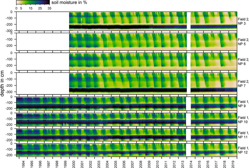
3532                                                                                      M. Merk et al.: Deep desiccation of soils

Appendix A: Supplemental figures

Figure A1. Time series of soil moisture measurements at the test site near Karlsruhe, Germany. Measurements on Field 2 are available from
2000 onward. No measurements were taken during the first half of the year 2014.

Figure A2. Monthly averages of usable field capacity calculated at five selected weather stations (DWD Climate Data Center, 2020). Val-
ues were computed by the agrometeorological model AMBAV. The model calculates soil moisture under grass with sandy loam. The soil
sandy loam has a wilting point of 13 volumic% and a field capacity of 37 volumic%. Further model input parameters are hourly values of
temperature, dew point, wind speed, precipitation, global radiation and reflected long-wave radiation.

Hydrol. Earth Syst. Sci., 25, 3519–3538, 2021                                           https://doi.org/10.5194/hess-25-3519-2021
M. Merk et al.: Deep desiccation of soils                                                                                          3533

Figure A3. Potential and real evapotranspiration at five selected weather stations (DWD Climate Data Center, 2020).

Figure A4. Results
                h of individual
                      i         linear regressions for soil moisture measurements in the recultivation layer, expressed as change in soil
moisture content %a−1 .

https://doi.org/10.5194/hess-25-3519-2021                                            Hydrol. Earth Syst. Sci., 25, 3519–3538, 2021
3534 M. Merk et al.: Deep desiccation of soils Figure A5. Results of modeling soil moisture with Rbeast. (a) Trend component of the soil moisture time series. (b) Probability of a change point in the trend component. (c) Amplitude of annual seasonality derived from the seasonal component. (d) Probability of a change point in the seasonality component. Hydrol. Earth Syst. Sci., 25, 3519–3538, 2021 https://doi.org/10.5194/hess-25-3519-2021
M. Merk et al.: Deep desiccation of soils                                                                 3535

Figure A6. Seasonal component of the soil moisture time series.

https://doi.org/10.5194/hess-25-3519-2021                         Hydrol. Earth Syst. Sci., 25, 3519–3538, 2021
3536                                                                                         M. Merk et al.: Deep desiccation of soils

Data availability. The data that support the findings of this study        378, 179–204, https://doi.org/10.1016/j.jhydrol.2009.08.013,
are available from the authors upon reasonable request.                    2009.
                                                                         Augenstein, M., Goeppert, N., and Goldscheider, N.: Char-
                                                                           acterizing soil water dynamics on steep hillslopes from
Author contributions. Markus Merk together with Nico Goldschei-            long-term lysimeter data, J. Hydrol., 529, 795–804,
der and Nadine Goeppert developed the concept of the study, for-           https://doi.org/10.1016/j.jhydrol.2015.08.053, 2015.
mulated research questions and discussed methods of data evalua-         Beck, H. E., Zimmermann, N. E., McVicar, T. R., Vergopolan, N.,
tion. Data curation, formal analysis of the data and visualization of      Berg, A., and Wood, E. F.: Present and future Köppen-Geiger
the results were done by Markus Merk and discussed by all the au-          climate classification maps at 1-km resolution, Scientific Data,
thors. The structure of the study was discussed by all authors and the     5, 180214, https://doi.org/10.1038/sdata.2018.214, 2018.
manuscript written by Markus Merk. The manuscript was reviewed,          Berger, K. U.: On the current state of the Hydrologic Evaluation of
edited and finally approved by all the authors.                            Landfill Performance (HELP) model, Waste Manage., 38, 201–
                                                                           209, https://doi.org/10.1016/j.wasman.2015.01.013, 2015.
                                                                         D’Odorico, P., Caylor, K., Okin, G. S., and Scanlon, T. M.: On soil
Competing interests. The authors declare that they have no conflict        moisture–vegetation feedbacks and their possible effects on the
of interest.                                                               dynamics of dryland ecosystems, J. Geophys. Res.-Biogeo., 112,
                                                                           G04010, https://doi.org/10.1029/2006JG000379, 2007.
                                                                         Dorigo, W., Wagner, W., Albergel, C., Albrecht, F., Balsamo, G.,
                                                                           Brocca, L., Chung, D., Ertl, M., Forkel, M., Gruber, A., Haas, E.,
Acknowledgements. We would like to thank Andreas Hoetzel from
                                                                           Hamer, P. D., Hirschi, M., Ikonen, J., de Jeu, R., Kidd, R., La-
the AfA Karlsruhe. We thank all persons who worked on this project
                                                                           hoz, W., Liu, Y. Y., Miralles, D., Mistelbauer, T., Nicolai-Shaw,
during the past 3 decades, doing maintenance on the measurement
                                                                           N., Parinussa, R., Pratola, C., Reimer, C., van der Schalie, R.,
systems and the lysimeters, conducting the measurements with the
                                                                           Seneviratne, S. I., Smolander, T., and Lecomte, P.: ESA CCI Soil
neutron probe, recording and curating the data, and thereby cre-
                                                                           Moisture for improved Earth system understanding: State-of-the
ating a rich treasure of data which we could base this work on.
                                                                           art and future directions, Remote Sens. Environ., 203, 185–215,
We are grateful for the funding we received from the city of Karl-
                                                                           https://doi.org/10.1016/j.rse.2017.07.001, 2017.
sruhe during the monitoring program. We thank Gary Witherall for
                                                                         Duethmann, D. and Blöschl, G.: Why has catchment evap-
the speedy language editing. We acknowledge support by the KIT-
                                                                           oration increased in the past 40 years? A data-based
Publication Fund of the Karlsruhe Institute of Technology.
                                                                           study in Austria, Hydrol. Earth Syst. Sci., 22, 5143–5158,
                                                                           https://doi.org/10.5194/hess-22-5143-2018, 2018.
                                                                         DWD Climate Data Center: Calculated daily values for differ-
Financial support. We were funded by the city of Karlsruhe during          ent characteristic elements of soil and crops, available at:
the monitoring program.                                                    ftp://opendata.dwd.de/climate_environment/CDC/derived_
                                                                           germany/soil/daily/historical/ (last access: 7 April 2020), 2020.
The article processing charges for this open-access                      DWD Climate Data Center (CDC): Historical daily pre-
publication were covered by the Karlsruhe Institute                        cipitation observations for Germany, available at:
of Technology (KIT).                                                       ftp://opendata.dwd.de/climate_environment/CDC/observations_
                                                                           germany/climate/daily/more_precip/historical/ (last access:
                                                                           26 March 2020), 2020.
Review statement. This paper was edited by Natalie Orlowski and          Evett, S. R. and Steiner, J. L.: Precision of Neutron Scat-
reviewed by Katrin Schneider and Jannis Groh.                              tering and Capacitance Type Soil Water Content Gauges
                                                                           from Field Calibration, Soil. Sci. Soc. Am. J., 59, 961–968,
                                                                           https://doi.org/10.2136/sssaj1995.03615995005900040001x,
                                                                           1995.
References                                                               Evett, S. R., Schwartz, R. C., Howell, T. A., Louis Baumhardt,
                                                                           R., and Copeland, K. S.: Can weighing lysimeter ET represent
Abichou, T., Liu, X., and Tawfiq, K.: Design Considera-                    surrounding field ET well enough to test flux station measure-
  tions for Lysimeters Used to Evaluate Alternative Earthen                ments of daily and sub-daily ET?, Adv. Water Resour., 50, 79–
  Final Covers, J. Geotech. Geoenviron., 132, 1519–1525,                   90, https://doi.org/10.1016/j.advwatres.2012.07.023, 2012.
  https://doi.org/10.1061/(ASCE)1090-0241(2006)132:12(1519),             Gerlach, A.: Wasserbilanzierung der Oberflächen-Abdichtung
  2006.                                                                    von Deponien unter Verwendung mathematischer Bi-
Albergel, C., Zheng, Y., Bonan, B., Dutra, E., Rodríguez-                  lanzierungsmodelle, Dissertation, Universität Karlsruhe,
  Fernández, N., Munier, S., Draper, C., de Rosnay, P., Muñoz-             Karlsruhe, https://doi.org/10.5445/IR/1000006087, 2007.
  Sabater, J., Balsamo, G., Fairbairn, D., Meurey, C., and Cal-          Goss, M. J., Ehlers, W., and Unc, A.: The role of lysime-
  vet, J.-C.: Data assimilation for continuous global assessment of        ters in the development of our understanding of processes
  severe conditions over terrestrial surfaces, Hydrol. Earth Syst.         in the vadose zone relevant to contamination of groundwa-
  Sci., 24, 4291–4316, https://doi.org/10.5194/hess-24-4291-2020,          ter aquifers, Phys. Chem. Earth, Parts A/B/C, 35, 913–926,
  2020.                                                                    https://doi.org/10.1016/j.pce.2010.06.004, 2010.
Allaire, S. E., Roulier, S., and Cessna, A. J.: Quantifying preferen-
  tial flow in soils: A review of different techniques, J. Hydrol.,

Hydrol. Earth Syst. Sci., 25, 3519–3538, 2021                                              https://doi.org/10.5194/hess-25-3519-2021
You can also read