Oceanographic Drivers of Cuvier's (Ziphius cavirostris) and Sowerby's (Mesoplodon bidens) Beaked Whales Acoustic Occurrence along the Irish Shelf ...
←
→
Page content transcription
If your browser does not render page correctly, please read the page content below
Journal of
               Marine Science
               and Engineering

Article
Oceanographic Drivers of Cuvier’s (Ziphius cavirostris) and
Sowerby’s (Mesoplodon bidens) Beaked Whales Acoustic
Occurrence along the Irish Shelf Edge
Cynthia Barile * , Simon Berrow                    and Joanne O’Brien

                                          Marine and Freshwater Research Centre (MFRC), Galway-Mayo Institute of Technology (GMIT),
                                          H91 T8NW Galway, Ireland; simon.berrow@gmit.ie (S.B.); joanne.obrien@gmit.ie (J.O.)
                                          * Correspondence: cynthia.barile94@gmail.com

                                          Abstract: Cuvier’s and Sowerby’s beaked whales occur year-round in western Irish waters, yet
                                          remain some of the most poorly understood cetaceans in the area. Considering the importance of the
                                          area for anthropogenic activities and the sensitivity of beaked whales to noise, understanding their
                                          ecology is essential to minimise potential overlaps. To this end, fixed bottom-mounted autonomous
                                          acoustic recorders were deployed at 10 stations over four recording periods spanning from May
                                          2015 to November 2016. Acoustic data were collected over 1934 cumulative days, for a total of
                                          7942 h of recordings. To model the probability of presence of Cuvier’s and Sowerby’s beaked
                                          whales in the area as a function of oceanographic predictors, we used Generalised Additive Models,
                                          fitted with Generalised Estimating Equations to deal with temporal autocorrelation. To reflect prey
                                          availability, oceanographic variables acting as proxies of primary productivity and prey aggregation

                                   processes such as upwelling events and thermal fronts were selected. Our results demonstrated
                                          that oceanographic variables significantly contributed to the occurrence of Cuvier’s and Sowerby’s
Citation: Barile, C.; Berrow, S.;
O’Brien, J. Oceanographic Drivers of
                                          beaked whales (p-values between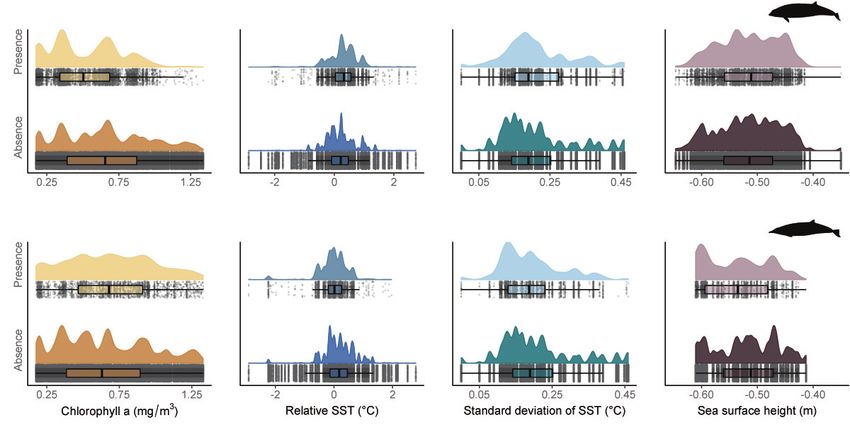
J. Mar. Sci. Eng. 2021, 9, 1081                                                                                           2 of 18

                                  odontocete species to emit frequency modulated clicks [10]. The spectral characteristics
                                  of Cuvier’s [10,11] and Sowerby’s beaked whales [12] (focal species of this study) have
                                  been previously described in the literature and their uniqueness allow reliable species
                                  discrimination.
                                        The slopes of the Irish Atlantic Margin, an area comprising waters to the west of
                                  the continental shelf, is an ideal candidate habitat for beaked whales, interspersed with
                                  canyons and troughs [13]. Together with a complex topography, the area is subject to
                                  complex oceanographic and hydrographic processes which combined, make it one of the
                                  most biologically productive regions in the northeast Atlantic [13]. Frontal systems, large
                                  eddies, upwelling and downwelling conditions have been recorded in the area [14–16]. Such
                                  events enhancing the local productivity propagate through the foodweb and determine
                                  the availability of prey items and in turn the occurrence of larger predators [13]. Many
                                  cephalopod species have indeed been recorded in the region [17,18], offering feeding
                                  opportunities to beaked whale species.
                                        Out of six beaked whale species recorded in the northeast Atlantic, five have been
                                  reported in Irish waters to date. Northern bottlenose and Cuvier’s beaked whales are
                                  the most frequently sighted and stranded species [19] and some speculate that the latter
                                  might be breeding in Irish waters [20]. Sowerby’s beaked whales (Mesoplodon bidens) have
                                  been sighted and found stranded on multiple occasions, but the recent sightings of calves
                                  during a survey on the shelf edge strongly suggest that Sowerby’s beaked whales could be
                                  breeding in the area [19]. True’s beaked whales (Mesoplodon mirus) have been identified in
                                  more than a dozen stranding events with individuals of different sizes, including a mother
                                  and a calf [21] but are likely to have been sighted at sea on a single occasion only [13].
                                  Gervais’ beaked whales (Mesoplodon europaeus) are known from a single stranding [22].
                                  Finally, Baird’s beaked whales stranded on two occasions in UK waters but have not yet
                                  been recorded in Ireland [19].
                                        Despite the diversity of the beaked whale family, we still know relatively little on
                                  many species. Most of the long-term research efforts have been focused on four species [2],
                                  including multiple populations of Cuvier’s (Ziphius cavirostris) and Blainville’s beaked
                                  whales (Mesoplodon densirostris) [23–25], as well as single populations of northern bot-
                                  tlenose (Hyperoodon ampullatus) [26] and Baird’s beaked whales (Berardius bairdii) [27]. For
                                  other species, information often relies on beach-cast individuals or skeletal remains [28,29].
                                  Beaked whales, as all other cetacean species, are listed under the Annex IV of the European
                                  Union (EU) Habitats Directive (EU-COM, 1992), entitling them to a strict level of protection.
                                  However, “to implement meaningful species conservation measures under the Directive, a
                                  good knowledge of each species (range, occurrences, biology, ecology, threats and sensi-
                                  tivity, conservation needs, etc.) is a conditio sine qua non” [30]. Enhancing the knowledge
                                  on distribution, abundance, habitat use and sensitivity to relevant threats can therefore be
                                  considered a priority.
                                        The lack of information on beaked whales is even more alarming given that they
                                  have been identified as sensitive to anthropogenic noise [25,31,32]. In particular, mid-
                                  frequency military sonar exposure has been blamed in many atypical mass stranding
                                  events [33–35] and shown to induce behavioural changes [25,36,37]. Although much
                                  less studied, other intense sound sources such as shipping and seismic airguns are of
                                  concern [34,38,39]. In 2018, the western Irish and British coasts experienced the largest
                                  unusual mortality event of beaked whales recorded globally. While causes of death could
                                  not be confirmed, lesions were not inconsistent with acoustic traumas [40]. Three similar
                                  stranding events of a lesser magnitude have occurred in the area over a decade [40,41]. The
                                  Irish Atlantic Margin is thought to hold significant hydrocarbon resources, placing the area
                                  at the frontline of increased noise levels, with seismic prospects expected to multiply [42].
                                  It becomes evident that investigating the spatio-temporal overlap between beaked whales
                                  and such anthropogenic stressors is important to devise strategies to manage and minimise
                                  potential risks.
J. Mar. Sci. Eng. 2021, 9, 1081 3 of 18
Here, we used data collected along the Irish Atlantic Margin over two years using
bottom-mounted recorders to examine the occurrence of foraging Cuvier’s and Sowerby’s
beaked whales, in relation to oceanographic drivers susceptible to influence the distri-
bution of prey items. Direct prey-related information is generally difficult to access and
environmental variables acting as proxies are often used instead [43] and allow an indirect
examination of the habitat preferences of predators [5,44,45]. Little is known about the
influence of oceanographic variables on the presence of Cuvier’s and Sowerby’s beaked
whales. This study explores the largest acoustic dataset collected using static devices in
Europe to date, to provide information on factors which could influence the presence and
distribution of those elusive species.
2. Materials and Methods
2.1. Data Collection
Acoustic data were collected along the edge of the continental shelf off western Ireland
using Autonomous Multichannel Acoustic Recorders (AMARs; JASCO Applied Sciences)
over four recording periods spanning from May 2015 to November 2016 (Table 1). The
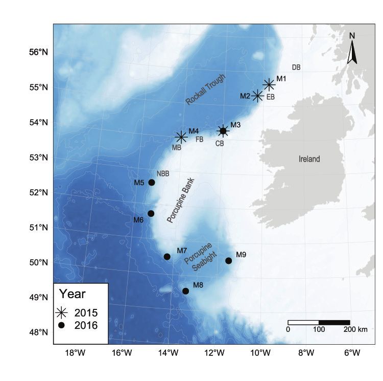
devices were suspended 15 m above the seafloor at four locations in 2015 (M1–M4) and six
in 2016 (M3, M5-M9; Figure 1 and Table 1), at an average operating depth of approximately
1800 m.
Figure 1. Location and year of deployment of the AMARs deployed along the Irish Atlantic Margin.
CB: Colm Basin, DB: Donegal Basin, EB: Erris Basin, FB: Fursa Basin, MB: Macdara Basin, NBB: North
Brona Basin.J. Mar. Sci. Eng. 2021, 9, 1081 4 of 18
Table 1. Location, depth, operation period, daily and overall recording durations of AMARs deployed at nine stations off western Ireland in 2015 and 2016.
Latitude Longitude Depth Recording Duration Per Day Recording Period Total Recording Time
Mooring (°N) (°W) (m)
Start End (Hours) (Cumulative Days) (Hours)
55.6302 −9.7302 1600 8 May 2015 22 August 2015 6.5
M1 214 1391
55.6323 −9.7252 1620 29 August 2015 13 December 2015 6.5
55.3018 −10.3084 1995 8 May 2015 22 August 2015 6.5
M2 214 1391
55.3011 −10.3037 1971 29 August 2015 13 December 2015 6.5
54.2513 −11.9940 1850 30 August 2015 14 December 2015 6.5 107 696
M3
54.2502 −11.9926 1770 24 March 2016 29 June 2016 2.6 98 255
54.0014 −14.0424 1920 7 May 2015 20 August 2015 6.5
M4 212 1378
54.0015 −14.0429 1944 30 August 2015 13 December 2015 6.5
52.6225 −15.3045 1752 21 March 2016 10 July 2016 2.6
M5 227 590
52.6221 −15.3046 1750 10 July 2016 2 November 2016 2.6
51.7226 −15.2077 1765 20 March 2016 11 July 2016 2.6
M6 210 546
51.7245 −15.2342 1745 11 July 2016 15 October 2016 2.6
50.5096 −14.3124 1750 19 March 2016 11 July 2016 2.6
M7 230 598
50.5085 −14.3150 1750 11 July 2016 3 November 2016 2.6
49.5477 −13.3730 1760 19 March 2016 9 August 2016 2.6
M8 122 598
49.5478 −13.3723 1760 9 August 2016 3 November 2016 2.6
M9 50.4867 −11.4963 1530 2 June 2016 4 November 2016 3.2 156 499J. Mar. Sci. Eng. 2021, 9, 1081 5 of 18
In 2015, AMARs were equipped with omnidirectional HTI-99-HF hydrophones (High
Tech Inc., Harrison County, MI, USA, −164 dB re 1 V/µPa sensitivity), operating on 8-min
duty cycles and recording for 130 sec during each cycle. In 2016, omnidirectional M36-
V35-100 hydrophones (GeoSpectrum Technologies Inc., Canada, −165 dB re 1 V/µPa
sensitivity) were used, operating on 8-min or 15-min duty cycles, with recording durations
of 64 to 97 s per cycle. To record high-frequency beaked whale clicks, high sampling rate
channels (250 kHz) with a 16-bit resolution, a spectral noise floor of 35 dB re 1 µPa2 /Hz
and a nominal ceiling of 171 dB re 1 µPa were used. The instruments were retrieved using
acoustic releases and recordings stored on internal solid-state flash memory.
2.2. Beaked Whale Detections
To identify odontocete clicks, acoustic recordings were processed using the combi-
nation of a custom automated click detector and classifier developed by JASCO Applied
Sciences [46]. The algorithm is based on the zero-crossings in the acoustic time series
(i.e., the rapid oscillations of clicks above and below the signal’s normal level). Firstly,
a high-pass filter was applied to the raw data to remove the energy below 8 kHz. This
allows the energy from cetacean clicks to pass while removing that of other sources such as
cetacean tonal calls, shrimps and vessels. A Teager-Kaiser energy detector [47] was then
applied, to detect potential clicks. For each detected click, three classification parameters
were extracted: (1) the number of zero-crossings within the click, (2) the median time
separation between zero-crossings and (3) the slope of the change in time separation be-
tween zero-crossings. This last parameter is particularly helpful for beaked whales, which
clicks can be identified by a frequency increase (i.e., upsweep). Those parameters were
compared to a beaked whale click template library and Mahalanobis distances [48] were
computed (i.e., the characteristics of recorded clicks were compared to typical distributions
of click characteristics). Each click was classified as the species which corresponded the
lowest value.
To verify the performance of the automatic detector, experienced bio-acoustic analysts
carried out a visual and aural review of a selection of acoustic files using PAMlab (JASCO
Applied Sciences). To be representative, the selection process was standardised, covering
various conditions (i.e., time of year and day, number of automatic detections, number
of species detected). The identification of beaked whale clicks was based on previous
descriptions available in the literature [10–12]. The validation process evaluated the
performance of the automatic detector in identifying at least one click in an acoustic
file, but did not indicate whether all or only a portion of the recorded clicks were detected.
To compare the manual and automatic detection results, a maximum likelihood estimation
algorithm was used to determine the detection threshold, i.e., the minimum number of
automated detections necessary for a species to be considered as present in the investigated
file, that maximised the F-score (F), calculated as follows:
(1 + β2 ) P ∗ R TP TP
F= 2
;P = ;R = (1)
(β )P + R TP + FP TP + FN
where the precision (P; proportion of accurate detections) and recall (R; proportion of
recorded clicks automatically detected) indices are calculated based on the proportion of
clicks correctly identified (true positives; TP), incorrectly identified (false positive; FP), or
missed (false negatives; FN). Hence, presence/absence data were used and the species of
interest was considered absent in acoustic files in which the number of automatic detections
failed to meet the detection threshold. The procedure carried out has been described
thoroughly by Kowarski et al. [46]. Precision was prioritised over recall throughout the
process to maximise the reliability of the results.J. Mar. Sci. Eng. 2021, 9, 1081 6 of 18
2.3. Environmental Variables
The selected oceanographic variables were comprised of chlorophyll a concentration
(chla in mg/m3 ), standard deviation of sea surface temperature (sdSST in ◦ C), mean relative
SST (relSST in ◦ C) and sea surface height (SSH in m). Static variables (e.g., depth, slope
aspect) were not relevant in this study because of the lack of variability inherent to the
use of static recorders. As means to account for latitudinal differences in detection rates,
“mooring ID” was included as an additional variable.
The chla concentration was selected as an indicator of primary productivity and
phytoplankton biomass at the surface. Data was gathered by the Moderate Resolution
Imaging Spectroradiometer (MODIS) aboard NASA’s Aqua Spacecraft and accessed from
NOAA CoastWatch program website (http://coastwatch.pfeg.noaa.gov/index.html, ac-
cessed on 2 February 2021) using the R [49] package ’rerddapXtracto’ [50]. Given the
predatory nature of beaked whale cephalopod preys, a temporal lag of about 3 to 4 months
is expected for peaks in primary productivity to translate into increases in cephalopod
biomass [44,45,51]. Hence, daily mean chla concentration was averaged over the 90 days
preceding each recording date [44,45].
The sdSST and relSST were used as proxies for frontal activity and upwelling, respec-
tively, processes influencing the availability and concentration of cephalopods [44,45]. We
used SST data from the Pathfinder Version 5.3 dataset, collected by the Advanced Very
High Resolution Radiometer (AVHRR) aboard NOAA’s Polar Operational Environmen-
tal Satellites (POES) and pre-processed by the NASA’s SeaWiFS Data Analysis System
(SeaDAS). The relSST was calculated as the difference in SST between each recording
station and the average across the study area (defined as 52.5◦ –57◦ N, 9◦ –17◦ W in 2015 and
48◦ –56◦ N, 11◦ –17◦ W in 2016) for the corresponding month. Finally, we used SSH data
from the HYCOM (HYbrid Coordinate Ocean Model) data assimilative system. SST and
SSH data were accessed from NOAA CoastWatch program website using the R package
’rerddapXtracto’.
Choosing an arbitrary scale to investigate the significance of environmental processes
can lead to contradictions, given that relationships between top predators and environmen-
tal features depend on the scales considered [51]. To work around this issue, we preferred a
multi-scale approach, by which variables were tested under different spatio-temporal scales.
For SSH data, both weekly and monthly averages were considered at spatial resolutions of
0.25 × 0.25◦ and 0.50 × 0.50◦ . Due to missing values in SST data, monthly averages only
were evaluated for sdSST and relSST, at different spatial scales (0.20 × 0.20◦ ; 0.30 × 0.30◦
and 0.50 × 0.50◦ for Cuvier’s beaked whales, 0.10 × 0.10◦ ; 0.20 × 0.20◦ ; 0.30 × 0.30◦ and
0.50 × 0.50◦ for Sowerby’s beaked whales). Those same spatial scales were considered
for chla. The finest spatial resolution at which the covariates were considered was of
0.10 × 0.10◦ and 0.20 × 0.20◦ for Sowerby’s and Cuvier’s beaked whales, respectively.
This decision related to the maximum detection range of the signals of interest in the
area, predicted to be smaller for Sowerby’s (4 km) than for Cuvier’s beaked whale clicks
(14 km) [19,46]. Relationships between detections and environmental conditions could be
concealed if detection ranges exceed the scale of analysis [52].
2.4. Data Analysis
To investigate the relationships between the oceanographic parameters described
above and Sowerby’s and Cuvier’s beaked whales presence/absence (response vari-
able), we used a generalised additive model (GAM) framework [53]. To this end, pres-
ence/absence data and values for the environmental variable of interest were associated
with each single acoustic file (recorded every 8 min to 15 min) and input into a single model
for each species, all sites combined. Although investigating relationships on a site-by-site
basis would have been ideal to eliminate potential bias associated with the location of
each recorder, the lack of variability in oceanographic variables at each individual site did
not allow such a fine-scale analysis. To counteract this limitation and account for spatial
differences in detection rates in this data shown by Kowarski et al. (2018) [46], “mooringJ. Mar. Sci. Eng. 2021, 9, 1081 7 of 18
ID” was added to the models as a categorical variable. All steps of data visualisation and
analysis were performed using scripts in R (version 4.0.3 [49]).
GAMs are widely used in modelling cetacean habitat and distribution, and allow the
investigation of non-linear cetacean-habitat relationships by replacing linear functions of
the covariates by smoothing functions [43,54]. However, significant temporal autocorrela-
tion of the residuals was revealed here by autocorrelation function plots and represents a
violation of GAM assumptions. To address this issue, we have used generalised estimating
equations (GEE), following the methodology in Pirotta et al. (2011) [45] to obtain so-called
GEE-GAMs. This strategy consists of grouping successive data points in independent
blocks and fitting a correlation structure within each block [55]. The temporal dependence
is expected to decrease with time, so an autoregressive order-1 (AR-1) covariance structure
was used here [56]. Multicollinearity between explanatory variables was tested using the
variance inflation factor (VIF). Binomial GEE-GLMs (generalised linear models) with a
log-link function were fitted using the R library ’geepack’ [57]. The ’splines’ library was
used to incorporate B-splines, thus extending to a GEE-GAM. All environmental covariates
were tested either as linear terms or as 1-dimensional smooth terms (4 degrees of freedom),
modelled as cubic B-splines with one internal knot at the average value of the covariate.
The categorical variable “mooring ID” was tested as a factor.
To select the best subset of variables, the quasi-likelihood under independence model
criterion (QIC) [58] was used to compare models in a stepwise selection. Model selection
can not be undertaken including the covariates under all their spatial and temporal scales
due to their strong collinearity. Thus, each variable was first tested at its different spatio-
temporal scales against the response variable to retain a single, optimal scale to be included
in the full model. This procedure resulted in comparing the QIC score of a null model with
those of a series of models containing the variable of interest at each of its available scales.
Once the most appropriate scale (spatial and temporal) and form (linear or smooth) were
found, a full model containing all selected covariates was fitted. A backwards stepwise
model selection was carried out by fitting a series of reduced models with all variables
but one. Covariates were taken out step by step, until none could be further removed
without increasing the QIC score. To determine the significance of each remaining covariate,
successive Wald’s tests were then carried out on the final model. Non-significant covariates
were removed one by one until all those remaining were significant (p < 0.05).
To evaluate model performance, presence-absence confusion matrices summarising
the model’s goodness-of-fit were used [59]. To build a confusion matrix, a cut-off prob-
ability value has to be selected, beyond which a prediction is considered a presence. To
select an appropriate cut-off, a Receiver Operating Characteristic (ROC) curve plotting the
proportion of correctly classified presences (i.e., sensitivity) versus the proportion of incor-
rectly classified presences (i.e., specificity) was computed using the R library ’ROCR’ [60].
The best cut-off was identified as the point where the distance between the ROC curve and
a 45◦ diagonal is maximised. In addition, the area under the curve (AUC) was computed
(’ROCR’ library) to assess overall model performance (the closer the AUC is to 1, the better
the model [61]).
To visualise the contribution of the predictors, partial residual plots of the estimated
relationships between the response and each of the variables were computed using the R
library ’ggplot2’ [62] and R-scripts coded by Pirotta et al. (2011) [45].
3. Results
3.1. Detector Performance
To verify the performance of the automatic click detectors, experienced analysts
manually reviewed 2830 acoustic files (1.09% of recordings) [46,63]. Across M1 to M8
the Cuvier’s beaked whale click classifier had a precision of 0.87 and a recall of 0.79 (F-
score = 0.86, Table 2). At M9, the recall value (0.80) was higher than the precision (0.48),
requiring the implementation of a classification threshold, which substantially optimised
the precision (post-threshold precision = 1, Table 2).J. Mar. Sci. Eng. 2021, 9, 1081 8 of 18
The performance of the Sowerby’s beaked whale click classifier was also satisfactory,
yielding a precision of 0.96 and a recall of 0.57–0.93 (F-score = 0.85–0.95, Table 2). It did not
require any optimisation because the precision was already higher than the recall, which
was our priority.
Table 2. Detector performance in detecting (recall, R) and correctly classifying (precision, P) beaked whale clicks. Data
from [46,63].
Species Mooring ID P R Classification Threshold Poptimised Roptimised Foptimised
M1–M8 0.87 0.79 1 0.87 0.79 0.86
Cuvier’s
M9 0.48 0.80 7 1.0 0.30 0.68
M1–M8 0.96 0.93 1 0.96 0.93 0.95
Sowerby’s
M9 0.96 0.57 1 0.96 0.57 0.85
3.2. Scale Selection
Explanatory variables were tested for multicollinearity, but VIF values remained
below 2 which allowed us to proceed and evaluate all four environmental variables of
interest in our models. Following our multi-scale approach, the appropriate spatial and
temporal scales (when appropriate) were selected for each oceanographic variable, taking
each species separately. As a result, chla and SSH data were retained on the 0.50 × 0.50◦
scale, sdSST on the 0.20 × 0.20◦ scale and relSST on the 0.30 × 0.30◦ scale (Table 3) in the
case of Cuvier’s beaked whales.
Table 3. Spatio-temporal scales under which chla concentration (mg/m3 ), sdSST (◦ C), relSST (◦ C)
and SSH (m) were retained for Cuvier’s and Sowerby’s beaked whale.
Species Covariate Scale Selected Covariate Median (Range)
chla 0.50 × 0.50◦ -90days 0.66 (0.18 to 1.3)
sdSST 0.20 × 0.20◦ -Monthly 0.19 (0.00 to 0.46)
Cuvier’s
relSST 0.30 × 0.30◦ -Monthly 0.22 (−2.9 to 2.7)
SSH 0.50 × 0.50◦ -Weekly −0.51 (−0.65 to −0.35)
chla 0.30 × 0.30◦ -90 days 0.62 (0.18 to 1.3)
sdSST 0.20 × 0.20◦ -Monthly 0.19 (0.00 to 0.46)
Sowerby’s
relSST 0.50 × 0.50◦ -Monthly 0.17 (−2.9 to 2.8)
SSH 0.25 × 0.25◦ -Monthly −0.51 (−0.61 to −0.41)
With regards to the temporal scales, weekly SSH averages were retained, while
monthly averages were retained for sdSST and relSST. For Sowerby’s beaked whales,
chla was retained on the 0.30 × 0.30◦ scale and SSH on the monthly 0.25 × 0.25◦ scale.
Similarly to Cuvier’s beaked whales, monthly sdSST averages on the 0.20 × 0.20◦ scale
were retained, but relSST was retained at a coarser spatial resolution of 0.50 × 0.50◦ .
3.3. General Observed Trends
Acoustic data were collected at four stations in the northern half of the shelf edge of
the Porcupine Bank from late spring (May) to early winter (December) 2015. Another five
stations were monitored in 2016 from early spring (March) to late fall (November) in the
southern half of the shelf edge of the Porcupine Bank and in the Porcupine Seabight (Figure
1 and Table 1). Exceptionally, M3 was monitored in 2016 due to equipment failure in the
first half of the sampling period in 2015. This represented a temporal coverage of 447 days
in total, across both years. Across all stations, 1790 cumulative days were acoustically
monitored. This resulted in a total of 7942 h of recordings from which click detections of
Cuvier’s and Sowerby’s beaked whales were extracted. Cuvier’s and Sowerby’s clicks
were detected in 2.6% and 1.1% of the total number of recordings (n = 260,210) and during
96% and 95% of the days monitored across both years (n = 447), respectively. Boxplots wereJ. Mar. Sci. Eng. 2021, 9, 1081 9 of 18
generated to visualise the ranges of the oceanographic variables of interest (under their
appropriate spatio-temporal scales—see Table 3) observed in both the absence and presence
of beaked whale click detections (Figure 2). Ranges and medians for those explanatory
variables are also given in Table 3.
When Cuvier’s beaked whale clicks were detected, observed values of chla were
lower than in the absence of detections (median = 0.49 mg/m3 vs. 0.65 mg/m3 , re-
spectively). The opposite tendency was observed for Sowerby’s beaked whales, with
higher chla values in the presence of click detections (median = 0.68 mg/m3 ) than in
their absence (median = 0.62 mg/m3 ). Monthly averages of relSST were higher in the
presence of Cuvier’s beaked whale click detections (median = 0.26 ◦ C) than in their absence
(median = 0.17 ◦ C). The opposite trend occurred with Sowerby’s beaked whale clicks,
with lower monthly relSST (median = 0.014 ◦ C) in the presence than in the absence of
detections (median = 0.17 ◦ C). For both species, the values of sdSST were very similar in the
absence or presence of click detections (median = 0.19 ◦ C). Finally, there was no noticeable
difference in SSH in the presence or absence of Cuvier’s beaked whale click detections
(median = −0.52 m). Regarding Sowerby’s beaked whales, the presence of click detections
seemed to be associated with lower SSH values (median = −0.54 m) than their absence
(median = −0.51 m).
Figure 2. Observed values of oceanographic variables in the presence and absence of Cuvier’s (first row) and Sowerby’s
(second row) beaked whale click detections: (a) chla concentration, (b) relative sea surface temperature (SST), (c) standard
deviation of SST and (d) sea surface height. Each variable is shown at the most appropriate scale, as determined by the
preliminary multi–scale approach (see Table 4).
3.4. Modelling Results
For Cuvier’s beaked whales, all oceanographic variables considered (chla, sdSST,
relSST and SSH) were retained as smooth terms (i.e., non-linear). The subsequent covariate
selection process, based on QIC scores and then on Wald’s tests, retained as final the model
containing all covariates which were considered, namely chla, sdSST, relSST, SSH and
mooring ID (p-values in Table 4). The confusion matrix suggested a capacity of the model
to correctly predict 83% of the presences and 60% of the absences, for an AUC of 0.77.J. Mar. Sci. Eng. 2021, 9, 1081 10 of 18
Table 4. Summary of model performance (AUC) and Wald’s test results for all significant covariates
in the final models. The order in which covariates are listed reflects their importance in the models.
Species AUC Covariate χ2 p-Value
Mooring ID 1255.7J. Mar. Sci. Eng. 2021, 9, 1081 11 of 18
0.30 ◦ C. Finally, the probability of detecting both species increased overall as SSH values
were increasing, so that it was the lowest when SSH values the most negative. However, the
wide confidence intervals in some cases (especially for Cuvier’s beaked whales) suggested
great caution should be taken in the interpretation of those observations.
Figure 4. Probability of presence of Cuvier’s (first row) and Sowerby’s (second row) beaked whale clicks modelled
as a smooth function of (a) chlorophyll a concentration, (b) relative sea surface temperature (SST), (c) standard devia-
tion of SST and (d) sea surface height. Rug plots (on x–axes) indicate actual data values. Shaded areas represent 95%
confidence intervals.
4. Discussion
This study combined acoustic data collected on an unprecedented scale in shelf-edge
waters off western Ireland [63,64], an important area for several deep diving cetacean
species. The exploitation of this large dataset already provided compelling evidence of
the importance of the area for Cuvier’s and Sowerby’s beaked whales for the first time,
highlighting their presence year-round [19,46,64]. To complement and build on those
recent findings, we showed here the importance of oceanographic drivers for Cuvier’s
and Sowerby’s beaked whales in this part of the northeast Atlantic. Specifically, chla
concentration, sdSST, relSST and SSH all significantly influenced the probability of click
detection for both species. By including a variable to account for spatial variation in
probabilities of detection, we also confirmed the latitudinal partitioning, different for
each species, as showed by Kowarski et al. (2018) [46]. Specifically, Cuvier’s beaked
whales seemed to be exploiting more southern locations along the continental shelf, while
Sowerby’s preferred northern locations. The low probabilities of detection at M9 (not
available in the latter study) also highlights the importance of the shelf edge in comparison
with waters to the east of the Porcupine Seabight.
Various conditions known to enhance the local productivity have been described in the
Irish Atlantic Margin and are likely to contribute to the aggregation of beaked whale prey.
Interspersed with canyon and trough systems, the area is also subject to several currents,
including the North Atlantic Current (NAC). The NAC creates large eddies in the Rockall
Trough and generates currents to the west of the Porcupine shelf [65]. Deep tidal currents
are present off the Porcupine Seabight and along slope regions [66]. The Shelf-Slope Front
is the most important front feature in the area (running along the upper continental slope to
the west of the Porcupine Bank) and is associated with the continuous Shelf Edge Current
(SEC) [14]. Furthermore, upwelling cyclonic and downwelling anticyclonic eddies have
been recorded along the Irish shelf break frontal zone [16,67]. If some seem to be temporary,
lasting up to seven days [67], some persist for hundreds of days [16]. Associated with theJ. Mar. Sci. Eng. 2021, 9, 1081 12 of 18
complex topography of the area, these oceanographic processes are likely to determine
prey availability and in turn, the distribution and abundance of cetacean species [13,68].
Habitat modelling has the potential to inform management strategies by identifying
environmental features influencing species distribution or abundance [8,43,69]. However,
the most influential factor is likely to be prey distribution [70,71]. These data are often
difficult to obtain, so environmental variables are often used as indicators of the actual
forces driving predators’ distribution [72,73]. Echolocation has been shown to be consistent
during deep foraging dives in Cuvier’s and Blainville’s beaked whales [7] and can safely
be assumed to be a crucial aspect of Sowerby’s as well as other beaked whale species’
foraging behaviour. Given the operating depth of the static recorders (average 1800 m), we
can consider the detections in this study to be a proxy for Cuvier’s and Sowerby’s beaked
whales’ foraging activity, making the investigation of the influence of prey aggregating
features particularly relevant.
Chlorophyll a concentration at the surface has been widely used as an indicator of
primary productivity in studies focusing on deep-diving cetaceans [5,8,44,74,75]. Our
results suggested a negative influence of chla on Cuvier’s and Sowerby’s beaked whale
foraging activity. Similar trends were reported by Correia et al. (2015) [74] but there is
no general consensus in the literature, with either opposite effects [5] or no significant
influence of chla [8,75]. The challenge of collecting data on such elusive species is reflected
in the literature, as many studies report on beaked whales as a functional group, rather
than on individual species [8,74]. This could explain contradictory findings, as influences
of chla could vary across individual species.
We used metrics reflecting the occurrence of upwelling events (relSST) and frontal
activity (sdSST) instead of absolute sea surface temperature. The results revealed that the
highest probabilities of Sowerby’s beaked whale click detections coincided with lower
relSST values, which could indicate upwelling events. With Cuvier’s however, detection
rates seemed to generally increase with warmer relSST. Thermal fronts contribute to
nutrient enhancement, affecting productivity and prey aggregation [51]. In several studies,
they have been positively correlated with sperm whale aggregations [72,76,77], a species
sharing a similar feeding ecology as beaked whales, targeting cephalopod species [78].
Here, Cuvier’s and Sowerby’s beaked whale detection rates were stable until sdSST values
of approximately 0.30 ◦ C, beyond which a negative relationship was observed. This
subsequent decline in detection rates with increasing frontal activity was unexpected given
the literature above but could be the result of a modelling artefact (e.g., influence of another
factor unaccounted for) and might not have any ecological significance. Nonetheless,
habitat modelling attempts on individual beaked whale species are scarce, which limited
our ability to compare our findings.
The sea surface height was significant and moderately important in models for both
species. The probability of detection of both Cuvier’s and Sowerby’s beaked whales was
minimal when the SSH was the most negative. In the North Atlantic, SSH is generally
depressed (i.e., negative values), which can reflect cyclonic eddies, associated with high
productivity due to the occurrence of upwelling events [79]. Relationships between SSH
and beaked whale presence have been reported previously, suggesting an association
between the presence of the whales and that of eddies and upwelling phenomena [74,80].
In particular, Correia et al. (2015) [74] found that peaks in the presence of beaked whales
corresponded with either high negative or high positive anomalies. However in our study,
only negative SSH values were observed, which makes comparisons difficult.
The selection of variables for analysis must remain parsimonious and should be the
result of a thorough reflection process and rely on an a priori knowledge on the area and
the species of interest [43,81]. The nature of the data used should also be considered and
justified the exclusion of topographic features in this study. The use of static recorders here
allowed great temporal coverage but limited spatial coverage, which made topographical,
static variables, uninformative, especially since similar habitats were monitored. Given the
latitudinal range of deployment, untangling effects of the topography itself from effectsJ. Mar. Sci. Eng. 2021, 9, 1081 13 of 18
due to the latitude on beaked whale detection rates would not have been possible. Despite
being more appropriate because of their temporal dynamism, the use of static recorders
also limited the range of values from oceanographic variables. Complementary models
would benefit from more extensive spatial coverage, to determine whether our results
would be confirmed or whether different trends would emerge.
Determining the relevant scales to represent indirect prey-predator relationships is
a central challenge in ecology [82]. The choice of which scales to investigate is however
directly linked to the data exploited and with acoustic data, detection ranges should not
exceed the scale of analysis [52]. In this study, the detection ranges were limited since
beaked whale clicks attenuate quickly given their ultrasonic nature [11,12]. Sound prop-
agation models in the area predicted detection ranges of 14 km and 4 km for Cuvier’s
and Sowerby’s beaked whale clicks, respectively, [46,63,64]. By following a multi-scale ap-
proach [83,84], we have confirmed the importance of evaluating different spatio-temporal
resolutions, with different variables being associated with beaked whale activity on dif-
ferent temporal and spatial scales. Although more strenuous, such a process is essential
if one hopes to decipher the dynamism of species distribution in relation to a constantly
changing environment [84]. We have found here that often, Cuvier’s and Sowerby’s beaked
whales foraging activity was predominantly associated with features on different scales.
Pinpointing the exact underlying ecological implications of these results is challenging but
are likely to reflect differences in those species’ ecology along the Irish Atlantic Margin.
Recently, using the same dataset, Kowarski et al. (2018) [46] suggested the existence of
a potential niche and latitudinal partitioning between those two beaked whale species,
most likely linked to prey distribution, which we have confirmed here. Sowerby’s prey
on smaller cephalopods than Cuvier’s beaked whales and fish is an important part of the
diet of the former [78]. Differences in prey preferences, capture techniques or foraging
strategies can therefore explain those findings.
This latitudinal partitioning could also be a confounding factor in the current study, by
introducing some bias with regards to the influence of oceanographic features, given that
all stations were pooled together. Furthermore, the fact that northern and southern stations
were not sampled within the same calendar year further complexifies interpretations.
Investigating site-by-site interactions could be revealing considering the topographical
diversity in the area, but the lack of variability in oceanographic conditions at each station
precluded such detailed analysis. Future investigations would most certainly benefit from
added spatial variability in conditions, which could be obtained by exploiting transect data
for example. However, even if acoustic methods are far more efficient to monitor such
species than visual methods, instruments towed just below the surface do not come close to
the capabilities of bottom-mounted devices in terms of beaked whale detection capabilities.
Overall, model performances were satisfactory but not optimal. For both species,
the performance in capturing presences was good (over 79% for both species), but the
model’s ability to correctly classify absences was lower (60% and 51% for Cuvier’s and
Sowerby’s, respectively). This is not surprising given the high detection rates throughout
the area. Nonetheless, the approach undertaken here is most likely an oversimplification of
the relationships between those whales and their environment, reinforced by potentially
unknown missed predictors, which can also explain some of the results that do not align
with the literature. Most of all, despite being relevant to represent factors influencing prey
availability, proxies are not as reliable or as informative as direct prey data [44], given
the important gap between physical processes and the top of the food chain, especially
for species feeding at great depths. Direct information about prey stocks is very difficult
to obtain, especially in challenging open seas and even more so when the species of
interest is of low commercial value [78]. Furthermore, despite allowing a certain amount of
flexibility, the use of remotely sensed data has limitations given that they only reflect surface
conditions. The translation of processes occurring at the surface to those at greater depths
is not clearly understood and sometimes controversial [51]. This is problematic when
using data from bottom-mounted instruments, collected at great depths. TechnologicalJ. Mar. Sci. Eng. 2021, 9, 1081 14 of 18
advances offer alternative solutions such as Autonomous Underwater Vehicles equipped
with multibeam sonar technologies, which can give valuable information on abundance and
distribution of prey species [85]. In general, multidisciplinary, holistic approaches collecting
data on both biotic and abiotic parameters simultaneously [86] are the way forward and
root themselves in a more ambitious ecosystem-based management strategy [87]. Despite
its limitations, this study gave an insight into the environmental preferences of Cuvier’s
and Sowerby’s beaked whales, on which very little is known. This study will therefore
serve as a point of reference for future investigations on habitat preferences for those
species worldwide. It also highlights the value of static acoustic monitoring techniques for
detecting those elusive species.
Author Contributions: Conceptualization, C.B., S.B. and J.O.; Data curation, C.B. and J.O.; Formal
analysis, C.B.; Funding acquisition, S.B. and J.O.; Investigation, S.B. and J.O.; Methodology, C.B.,
S.B. and J.O.; Project administration, S.B. and J.O.; Resources, S.B. and J.O.; Software, C.B.; Super-
vision, S.B. and J.O.; Validation, C.B. and J.O.; Visualization, C.B.; Writing—original draft, C.B.;
Writing—review & editing, C.B., S.B. and J.O. All authors have read and agreed to the published
version of the manuscript.
Funding: This research received no external funding.
Data Availability Statement: Restrictions apply to the availability of these data. Data for stations M1
to M8 are owned by the Irish Department of Communications, Climate Action and Environment and
requests for access to the raw acoustic data can be submitted to PADadmin@DCCAE.gov.ie. Data for
stations M9 are owned by Woodside Energy Ltd. (Perth, Australia) and the Galway-Mayo Institute
of Technology.
Acknowledgments: This research was part of the PhD study of C.B., funded by the Galway-Mayo
Institute of Technology (GMIT) and Woodside Energy Ltd. The data used in this study is part
of a Woodside Energy Ltd. study and the ObSERVE Acoustic project, intiated and funded by
the Department of Communications, Climate Action and Environment in partnership with the
Department of Culture, Heritage and the Gaeltacht under Ireland’s ObSERVE Programme. The
GMIT was the lead organization in both Woodside and ObSERVE. We thank all teams involved in
administration, management and data collection, including the Marine Institute for logistical support
and JASCO Applied Sciences for data processing.
Conflicts of Interest: The authors declare no conflict of interest. Funders were involved in the design
of the study, namely regarding temporal and spatial coverage. However, they did not interfere with
analysis, data interpretation or writing of the manuscript. In addition, JASCO Applied Sciences was
contracted by GMIT to provide acoustic recorders, analysis services, but did not have any additional
role in the study design, data collection, or decision to publish.
Abbreviations
The following abbreviations are used in this manuscript:
AMAR Autonomous Multichannel Acoustic Recorders
AUC Area Under the Curve
AVHRR Advanced Very High Resolution Radiometer
chla chlorophyll a
EU European Union
GAM Generalised Additive Model
GEE Generalised Estimating Equation
GLM Generalised Linear Model
MODIS Moderate Resolution Imaging Spectroradiometer
MSFD Marine Strategy Framework Directive
NAC North Atlantic Current
PAM Passive Acoustic Monitoring
POES Polar Operational Environmental SatellitesJ. Mar. Sci. Eng. 2021, 9, 1081 15 of 18
QIC Quasi-likelihood Independence model Criterion
relSST relative sea surface temperature
ROC Receiver Operating Characteristic
sdSST standard deviation of sea surface temperature
SeaDAS SeaWiFS Data Analysis System
SEC Shelf Edge Current
SSH Sea surface height
References
1. Yamada, T.K.; Kitamura, S.; Abe, S.; Tajima, Y.; Matsuda, A.; Mead, J.G.; Matsuishi, T.F. Description of a new species of beaked
whale (Berardius) found in the North Pacific. Sci. Rep. 2019, 9, 1–14. [CrossRef] [PubMed]
2. Hooker, S.K.; De Soto, N.A.; Baird, R.W.; Carroll, E.L.; Claridge, D.; Feyrer, L.; Miller, P.J.; Onoufriou, A.; Schorr, G.; Siegal, E.;
et al. Future directions in research on beaked whales. Front. Mar. Sci. 2019, 5, 514. [CrossRef]
3. Tepsich, P.; Rosso, M.; Halpin, P.N.; Moulins, A. Habitat preferences of two deep-diving cetacean species in the northern Ligurian
Sea. Mar. Ecol. Prog. Ser. 2014, 508, 247–260. [CrossRef]
4. Benoit-Bird, K.; Southall, B.; Moline, M.; Claridge, D.; Dunn, C.; Dolan, K.; Moretti, D. Critical threshold identified in the
functional relationship between beaked whales and their prey. Mar. Ecol. Prog. Ser. 2020, 654, 1–16. [CrossRef]
5. Giorli, G.; Neuheimer, A.; Copeland, A.; Au, W.W.L. Temporal and spatial variation of beaked and sperm whales foraging activity
in Hawai’i, as determined with passive acoustics. J. Acoust. Soc. Am. 2016, 140, 2333–2343. [CrossRef]
6. Quick, N.J.; Cioffi, W.R.; Shearer, J.M.; Fahlman, A.; Read, A.J. Extreme diving in mammals: First estimates of behavioural aerobic
dive limits in Cuvier’s beaked whales. J. Exp. Biol. 2020, 223, 1–6. [CrossRef]
7. Tyack, P.L.; Johnson, M.; Soto, N.A.; Sturlese, A.; Madsen, P.T. Extreme diving of beaked whales. J. Exp. Biol. 2006, 209, 4238–4253.
[CrossRef]
8. Rogan, E.; Cañadas, A.; Macleod, K.; Santos, M.B.; Mikkelsen, B.; Uriarte, A.; Van Canneyt, O.; Vázquez, J.A.; Hammond, P.S.
Distribution, abundance and habitat use of deep diving cetaceans in the North-East Atlantic. Deep Sea Res. Part II Top. Stud.
Oceanogr. 2017, 141, 8–19. [CrossRef]
9. Mellinger, D.K.; Stafford, K.M.; Moore, S.E.; Dziak, R.P.; Matsumoto, H. An overview of fixed passive acoustic observation
methods for Cetaceans. Oceanography 2007, 20, 36–45. [CrossRef]
10. Baumann-Pickering, S.; McDonald, M.A.; Simonis, A.E.; Solsona Berga, A.; Merkens, K.P.B.; Oleson, E.M.; Roch, M.A.;
Wiggins, S.M.; Rankin, S.; Yack, T.M.; et al. Species-specific beaked whale echolocation signals. J. Acoust. Soc. Am. 2013,
134, 2293–2301. [CrossRef]
11. Zimmer, W.M.X.; Johnson, M.P.; Madsen, P.T.; Tyack, P.L. Echolocation clicks of free-ranging Cuvier’s beaked whales (Ziphius
cavirostris). J. Acoust. Soc. Am. 2005, 117, 3919–3927. [CrossRef] [PubMed]
12. Cholewiak, D.; Baumann-Pickering, S.; Van Parijs, S. Description of sounds associated with Sowerby’s beaked whales (Mesoplodon
bidens) in the western North Atlantic Ocean. J. Acoust. Soc. Am. 2013, 134, 3905–3912. [CrossRef] [PubMed]
13. O’Cadhla, O.; Mackey, M.; Aguilar de Soto, N.; Rogan, E.; Connolly, N. Cetaceans and Seabirds of Ireland’s Atlantic Margin.
Volume II: Cetacean Distribution and Abundance. Technical Report, Irish Infracture Programme (PIP): Rockall Studies Group
Projects 98/6 and 00/13, Porcupine Studies Group Project P00/15 and Offshore Support Group Project 99/38, 2004. Available
online: https://www.ucc.ie/research/crc/publications/reports/Vol2_Cetaceans_Final.pdf (accessed on 28 July 2021).
14. Belkin, I.M.; Cornillon, P. Fronts in the world ocean’s large marine ecosystems. ICES CM 2007, 21, 1–33.
15. Dransfeld, L.; Maxwell, H.; Moriarty, M.; Nolan, C.; Kelly, E.; Pedreschi, D.; Slattery, N.; Connolly, P. North Western Waters Atlas,
3rd ed.; Marine Institute: Oranmore, Ireland, 2014.
16. Shoosmith, D.R.; Richardson, P.L.; Bower, A.S.; Rossby, H.T. Discrete eddies in the northern North Atlantic as observed by
looping RAFOS floats. Deep Sea Res. Part II Top. Stud. Oceanogr. 2005, 52, 627–650. [CrossRef]
17. Clarke, M.R. Oceanic cephalopod distribution and species diversity in the Eastern North Atlantic. Arquipel. Life Mar. Sci. 2006,
23A, 27–46.
18. Hastie, L.; Pierce, G.; Wang, J.; Bruno, I.; Moreno, A.; Piatkowski, U.; Robin, J. Cephalopods In The North-eastern Atlantic.
Oceanogr. Mar. Biol. Annu. Rev. 2009, 47, 111–190. [CrossRef]
19. Berrow, S.; Meade, R.; Marrinan, M.; Mckeogh, E.; Brien, J.O. First confirmed sighting of Sowerby’s beaked whale (Mesoplodon
bidens (Sowerby, 1804)) with calves in the Northeast Atlantic. Mar. Biodivers. Rec. 2018, 11, 1–5. [CrossRef]
20. Berrow, S. Biological diversity of cetaceans (whales, dolphins and porpoises) in Irish waters. Mar. Biodivers. Irel. Adjac. Waters
2001, 26, 115–120.
21. Hernandez-Milian, G.; Lusher, A.; O’Brian, J.; Fernandez, A.; O’Connor, I.; Berrow, S.; Rogan, E. New information on the diet of
True’s beaked whale (Mesoplodon mirus, Gray 1850), with insights into foraging ecology on mesopelagic prey. Mar. Mammal Sci.
2017, 33, 1245–1254. [CrossRef]
22. Bruton, T.; Cotton, D.; Enright, M. Gulf Stream Beaked Whale Mesoplodon Europaeus (Gervais). Ir. Nat. J. 1989, 23, 156.
23. Arranz, P.; Borchers, D.L.; De Soto, N.A.; Johnson, M.P.; Cox, M.J. A new method to study inshore whale cue distribution from
land-based observations. Mar. Mammal Sci. 2014, 30, 810–818. [CrossRef]J. Mar. Sci. Eng. 2021, 9, 1081 16 of 18
24. Coomber, F.; Moulins, A.; Tepsich, P.; Rosso, M. Sexing free-ranging adult Cuvier’s beaked whales (Ziphius cavirostris) using
natural marking thresholds and pigmentation patterns. J. Mammal. 2016, 97, 879–890. [CrossRef]
25. Falcone, E.A.; Schorr, G.S.; Watwood, S.L.; DeRuiter, S.L.; Zerbini, A.N.; Andrews, R.D.; Morrissey, R.P.; Moretti, D.J. Diving
behaviour of cuvier’s beaked whales exposed to two types of military sonar. R. Soc. Open Sci. 2017, 4, 1–21. [CrossRef] [PubMed]
26. O’Brien, K.; Whitehead, H. Population analysis of Endangered northern bottlenose whales on the Scotian Shelf seven years after
the establishment of a Marine Protected Area. Endanger. Species Res. 2013, 21, 273–284. [CrossRef]
27. Fedutin, I.D.; Filatova, O.A.; Mamaev, E.G.; Burdin, A.M.; Hoyt, E. Occurrence and social structure of Baird’s beaked whales,
Berardius bairdii, in the Commander Islands, Russia. Mar. Mammal Sci. 2015, 31, 853–865. [CrossRef]
28. MacLeod, C.; Mitchell, G. Key areas for beaked whales worldwide. J. Cetacean Res Manag. 2006, 7, 309–322.
29. Baird, R. Behavior and ecology of social odontocetes: Cuvier’s and Blainville’s beaked whales. In Ethology and Behavioral Ecology
of Toothed Whales and Dolphins, The Odontocetes; Wursig, B., Ed.; Springer: Berlin/Heidelberg, Germany, 2019. [CrossRef]
30. European Commission. Guidance Document on the Strict Protection of Animal Species of Community Interest under the Habitats
Directive 92/43/EEC. 2007. Available online: https://ec.europa.eu/environment/nature/conservation/species/guidance/pdf/
guidance_en.pdf (accessed on 28 July 2021).
31. Bernaldo de Quirós, Y.; Fernandez, A.; Baird, R.W.; Brownell, R.L.; Aguilar de Soto, N.; Allen, D.; Arbelo, M.; Arregui, M.;
Costidis, A.; Fahlman, A.; et al. Advances in research on the impacts of anti-submarine sonar on beaked whales. Proc. R. Soc. Biol.
Sci. 2019, 286, 1–9. [CrossRef] [PubMed]
32. Simonis, A.; Brownell, R.; Thayre, B.; Trickey, J.; Oleson, E.; Huntington, R.; Baumann-Pickering, S. Co-occurrence of beaked
whale strandings and naval sonar in the Mariana Islands, Western Pacific. Proc. Biol. Sci. 2020, 287, 1–10. [CrossRef] [PubMed]
33. Cox, T.M.; Ragen, T.J.; Read, A.J.; Vos, E.; Baird, R.W.; Balcomb, K.; Barlow, J.; Caldwell, J.; Cranford, T.; Crum, L.; et al.
Understanding the impacts of anthropogenic sound on beaked whales. J. Cetacean Res. Manag. 2006, 7, 177–187.
34. D’Amico, A.; Gisiner, R.C.; Ketten, D.R.; Hammock, J.A.; Johnson, C.; Tyack, P.L.; Mead, J. Beaked whale strandings and naval
exercises. Aquat. Mamm. 2009, 35, 452–472. [CrossRef]
35. Filadelfo, R.; Mintz, J.; Michlovich, E.; D’Amico, A.; Tyack, P.L.; Ketten, D.R. Correlating military sonar use with beaked whale
mass strandings: What do the historical data show? Aquat. Mamm. 2009, 35, 435–444. [CrossRef]
36. Joyce, T.; Durban, J.; Claridge, D.; Dunn, C.; Hickmott, L.; Fearnbach, H.; Dolan, K.; Moretti, D. Behavioral responses of satellite
tracked Blainville’s beaked whales (Mesoplodon densirostris) to mid-frequency active sonar. Mar. Mammal Sci. 2020, 36, 29–46.
[CrossRef]
37. Wensveen, P.J.; Isojunno, S.; Hansen, R.R.; Von Benda-Beckmann, A.M.; Kleivane, L.; Van Ijsselmuide, S.; Lam, F.P.A.; Kvadsheim,
P.H.; Deruiter, S.L.; Curé, C.; et al. Northern bottlenose whales in a pristine environment respond strongly to close and distant
navy sonar signals. Proc. R. Soc. B 2019, 286, 1–10. [CrossRef]
38. Aguilar Soto, N.; Johnson, M.; Madsen, P.T.; Tyack, P.L.; Bocconcelli, A.; Fabrizio Borsani, J. Does intense ship noise disrupt
foraging in deep-diving cuvier’s beaked whales (Ziphius cavirostris)? Mar. Mammal Sci. 2006, 22, 690–699. [CrossRef]
39. Cholewiak, D.; DeAngelis, A.I.; Palka, D.; Corkeron, P.J.; Van Parijs, S.M. Beaked whales demonstrate a marked acoustic response
to the use of shipboard echosounders. R. Soc. Open Sci. 2017, 4, 1–15. [CrossRef]
40. Brownlow, A.; Davsion, N.; Ten Doeschate, M.; Berrow, S.; Dagleish, M.; Deaville, R.; van Geel, N.; Hantke, G.; Jepson, P.;
Onoufriou, A.; et al. Deep trouble: Investigation into an unprecedented number of beaked whale strandings, eastern Atlantic,
July–October 2018. In Proceedings of the World Marine Mammal Science Conference, Barcelona, Spain, 8–12 December 2019.
41. Dolman, S.J.; Pinn, E.; Reid, R.J.; Barley, J.P.; Deaville, R.; Jepson, P.D.; O’Connell, M.; Berrow, S.; Penrose, R.S.; Stevick, P.T.; et al.
A note on the unprecedented strandings of 56 deep-diving whales along the UK and Irish coast. Mar. Biodivers. Rec. 2010, 3, 1–8.
[CrossRef]
42. Beck, S.; O’Connor, I.; Berrow, S.; O’Brien, J. Report Series No. 120. Assessment and Monitoring of Ocean Noise in Irish Waters; Envi-
ronmental Protection Agency: Dublin, Ireland, 2013; Number 101, p. 120. Available online: https://www.epa.ie/publications/
research/water/STRIVE-120---Assessment-and-Monitoring-of-Ocean-Noise-in-Irish-Waters.pdf (accessed on 28 July 2021).
43. Redfern, J.V.; Ferguson, M.C.; Becker, E.A.; Hyrenbach, K.D.; Good, C.; Barlow, J.; Kaschner, K.; Baumgartner, M.F.; Forney, K.A.;
Ballance, L.T.; et al. Techniques for cetacean—Habitat modeling. Mar. Ecol. Prog. Ser. 2006, 310, 271–295. [CrossRef]
44. Eguiguren, A.; Pirotta, E.; Cantor, M.; Rendell, L.; Whitehead, H. Habitat use of culturally distinct Galápagos sperm whale
Physeter macrocephalus clans. Mar. Ecol. Prog. Ser. 2019, 609, 257–270. [CrossRef]
45. Pirotta, E.; Matthiopoulos, J.; MacKenzie, M.; Scott-Hayward, L.; Rendell, L. Modelling sperm whale habitat preference: A novel
approach combining transect and follow data. Mar. Ecol. Prog. Ser. 2011, 436, 257–272. [CrossRef]
46. Kowarski, K.; Delarue, J.; Martin, B.; O’Brien, J.; Meade, R.; Cadhla, O.; Berrow, S. Signals from the deep: Spatial and temporal
acoustic occurrence of beaked whales off western Ireland. PLoS ONE 2018, 13, e0199431. [CrossRef] [PubMed]
47. Kaiser, J. On a simple algorithm to calculate the ’energy’ of a signal. In Proceedings of the International Conference on Acoustics,
Speech, and Signal Processing, Albuquerque, NM, USA, 3–6 April 1990; pp. 381–384. [CrossRef]
48. Mahalanobis, P.C. On the Generalized Distance in Statistics. Proc. Natl. Inst. Sci. India 1936, 2, 49–55.
49. Team, R.C. R: A Language and Environment for Statistical Computing; R Foundation for Statistical Computing: Vienna, Austria, 2018.
50. Mendelssohn, R. Package ’rerddapXtracto’. R Package Version 1.0.2., 2020. Available online: https://cran.r-project.org/web/
packages/rerddapXtracto/rerddapXtracto.pdf (accessed on 2 February 2021).You can also read