Landscape Connectivity and Suitable Habitat Analysis for Wolves (Canis lupus L.) in the Eastern Pyrenees - MDPI
←
→
Page content transcription
If your browser does not render page correctly, please read the page content below
sustainability

Article
Landscape Connectivity and Suitable Habitat
Analysis for Wolves (Canis lupus L.) in the
Eastern Pyrenees
Carla Garcia-Lozano 1 , Diego Varga 1, * , Josep Pintó 1        and Francesc Xavier Roig-Munar 2
 1    Geography Department, University of Girona, 17004 Girona, Spain; carla.garcia@udg.edu (C.G.-L.);
      josep.pinto@udg.edu (J.P.)
 2    Independent Researcher, 07760 Menorca, Spain; xiscoroig@gmail.com
 *    Correspondence: diego.varga@udg.edu; Tel.: +34-972-418-778

 Received: 6 May 2020; Accepted: 15 July 2020; Published: 17 July 2020

 Abstract: Over the last few decades, much of the mountain area in European countries has turned
 into potential habitat for species of medium- and large-sized mammals. Some of the occurrences
 that explain this trend are biodiversity protection, the creation of natural protected areas, and the
 abandonment of traditional agricultural activities. In recent years, wolves have once again been seen
 in forests in the eastern sector of the Pyrenees and the Pre-Pyrenees. The success or failure of their
 permanent settlement will depend on several factors, including conservation measures for the species,
 habitat availability, and the state of landscape connectivity. The aim of this study is to analyze the
 state of landscape connectivity for fragments of potential wolf habitat in Catalonia, Andorra, and on
 the French side of the Eastern Pyrenees. The results show that a third of the area studied constitutes
 potential wolf habitat and almost 90% of these spaces are of sufficient size to host stable packs.
 The set of potential wolf habitat fragments was also assessed using the probability of connectivity
 index (dPC), which analyses landscape connectivity based on graph structures. According to the
 graph theory, the results confirm that all the nodes or habitat fragments are directly or indirectly
 interconnected, thus forming a single component. Given the large availability of suitable habitat
 and the current state of landscape connectivity for the species, the dispersal of the wolf would be
 favorable if stable packs are formed. A new established population in the Pyrenees could lead to more
 genetic exchange between the Iberian wolf population and the rest of Europe’s wolf populations.

 Keywords: wolf (Canis lupus); Pyrenees; habitat suitability; ecological connectivity; landscape
 fragmentation; probability of connectivity (PC)

1. Introduction
     Policies aimed at conserving threatened species and ecosystems have been key in preventing their
further loss, resulting in the reversal of a trend that was leading to their extinction [1]. Nevertheless,
biodiversity has continued to decline on a global scale over recent decades [2]. Prior to the decline in
its populations, the wolf was widespread throughout Europe, especially where the presence of wild
ungulates allowed its survival [3]. Wolf attacks on livestock, and in some cases humans, were the
catalyst for its persecution, leading to the indiscriminate hunting of the species from at least the
sixteenth century onwards [4,5]. By the nineteenth and twentieth centuries, the species had been
drastically reduced in number and numerous local populations had been exterminated [6]. In France,
breeding populations of the wolf disappeared around 1940 [7] and in Catalonia the last wolf was
killed in the Eastern Pyrenees in 1945 [8]. However, the large carnivores still existing in Europe
today—the brown bear (Ursus arctos), the lynx (Lynx spp.), the wolverine (Gulo gulo), and the wolf

Sustainability 2020, 12, 5762; doi:10.3390/su12145762                       www.mdpi.com/journal/sustainability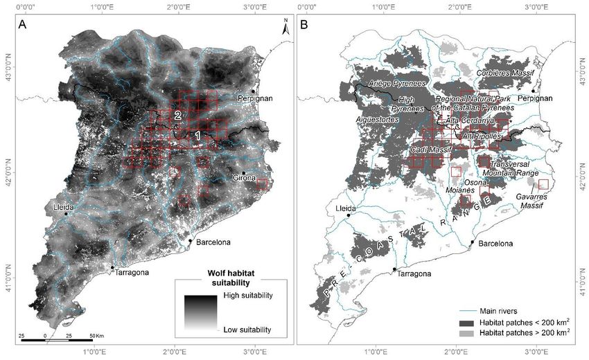
Sustainability 2020, 12, 5762 2 of 20
(Canis lupus)—all enjoy some form of protection in countries in the European Union. Chapron et al. [9]
consider the present coexistence of humans and large carnivores to be the outcome of joint conservation
efforts among several countries over the past three decades.
The establishment of networks of protected natural areas and environmental and socio-economic
changes in rural areas in recent decades has led to improvement in the quality of wildlife habitats.
The current dense forests in mountain locations and the wolf’s ability to colonize a diverse range of
anthropogenically modified habitats has favored the recovery of wolf populations in areas of Europe
where it had disappeared [10–12].
Chapron et al. [9] estimate that the current number of wolves in Europe exceeds 12,000 individuals,
excluding populations in Russia, Belarus, and the Ukraine. These populations are distributed in
nine different groups: Scandinavia (Norway and Sweden), the Karelian region (Finland), the central
European lowlands (Western Poland, Eastern Germany, and the Baltic regions), the Carpathians
(Slovakia, Czech Republic, Poland, Romania, Hungary, and Serbia), the Dinaric-Balkan region
(Slovenia, Croatia, Bosnia and Herzegovina, Montenegro, Albania, Servia, Greece, and Bulgaria),
the Alps (Italy, France, Switzerland, Austria, and Slovenia), the Italian Peninsula (Italy), North-West
Iberia (Spain and Portugal), and the Sierra Morena (Spain). However, the number of individuals in the
Sierra Morena population has been seriously reduced in the last few years and is consequently now
gravely threatened [13].
In the early twenty-first century, the presence of wolves was discovered on the Catalan side of
the Eastern Pyrenees, an area where the species had disappeared almost a century earlier. The first
scat samples were collected in Cadí-Moixeró Natural Park in 2000, although it was not until 2004 that
they were analyzed and the presence of the wolf confirmed [13,14]. According to Lampreave et al. [14],
the samples analyzed in the Catalan Pyrenees (Figure 1) up to 2011 confirm the presence of up to
thirteen different wolves, twelve males and one female. Samples collected on the French side showed
the presence of four different individuals in the Madres, Carlit-Peric, and Canigó Massifs, including
one female [15].
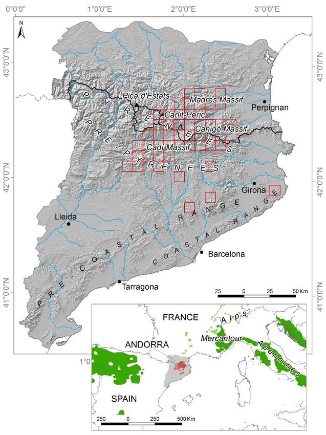
Contrary to expectation, the wolves that have reached the Eastern Pyrenees have not come from
existing populations on the Iberian Peninsula, but from the Italian Peninsula. Since the mid-seventies,
when the Italian government started to protect the species, the wolf has gradually dispersed from
Abruzzo National Park, situated in the central Apennines, to Mercantour Natural Park in the French
Alps (Figure 1), where it arrived in the early nineties [16] and was rapidly protected nationwide
according to French legislation. These populations quickly dispersed until reaching the Madres
Massif in the French Eastern Pyrenees in 1999, where months later they crossed to the Catalan
side (Figure 1) [14,17].
In recent years, the flow of lone wolves in the Eastern Pyrenees has been significantly reduced to
two or three individuals distributed in two areas with a permanent wolf presence (Figure 1) [13,18,19].
The Madres Massif and the Cadí Massif (Figure 1) are areas with temporary wolf presence, while in
March 2018 another lone wolf was killed on the road in the Catalan Coastal Mountain Range (Figure 1),
Les Gavarres massif, where there had been no sightings since its reappearance. According to these data,
nearly twenty different wolves in the Eastern Pyrenees, including two females, have been detected
since their arrival in 2000. Despite being considered a protected species, the French National Action
Plan for the Wolf (2013–2017) allows wolf hunting under some circumstances that, among other
ecological processes, may have con [20]. to the reduction of wolf flux over the last few years. In Spain,
the National Catalogue of Threatened Species (Catálogo Nacional de Especies Amenazadas) considers
the wolf to be a huntable species to the north of the Duero river, whereas it is strictly protected to the
south of it. In the case of Catalonia, the species does not have a protection status because it was not
present there when the Spanish protection law was enacted. In accordance with the European Habitats
Directive (Council Directive 92/43/EEC), the wolf is a species of priority community interest in the
whole of Europe, except for the local Spanish populations north of the Duero, those in the north of
Greece, and those all over Finland.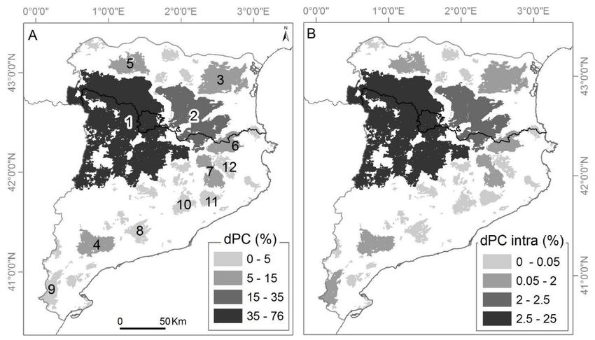
Sustainability 2020, 12, 5762                                                                                            3 of 20

     Loss of connectivity is the greatest threat to conserving biodiversity and maintaining ecological
Sustainability 2020, 12, x FOR PEER REVIEW                                                          3 of 20
functions in the landscape. Landscape connectivity facilitates the movement of species, genetic
exchange, and other ecological flows key to the survival of species and biodiversity conservation [21,22].
exchange, and other ecological flows key to the survival of species and biodiversity conservation
These functions acquire special relevance in the context of global environmental change, as species can
[21,22]. These functions acquire special relevance in the context of global environmental change, as
be forced to change their natural ranges.
species can be forced to change their natural ranges.

      Figure 1. Location of the area of study in Catalonia, Andorra, and the south-east of France. The red
      Figure
      squares1.indicate
                  Locationtheofpresence
                                the areaofofwolves
                                             study in     Catalonia,
                                                      at some         Andorra
                                                                time since       , and
                                                                             2000.     thewith
                                                                                    Areas  south-east of France.
                                                                                                permanent         The red
                                                                                                           wolf presence
      squares   indicate
      are located   aroundthe the
                               presence  of wolves
                                   Carlit-Peric       at some
                                                 region    and time   since 2000.
                                                                 the Canigó         AreasThe
                                                                                Massif.   with  permanent
                                                                                              small        wolf presence
                                                                                                    map shows    the wolf
      are  located around
      distribution   areas inthe   Carlit-Peric
                                southern         region
                                           Europe.      Theand
                                                             darkthegreen
                                                                      Canigó
                                                                           cellsMassif.  The
                                                                                  indicate thesmall map shows
                                                                                               permanent        the wolf
                                                                                                           occurrence   of
      distribution  areas   in southern   Europe.    The   dark  green  cells  indicate the permanent
      the wolf, and the light green cells indicate its temporary occurrence. Source: Data taken from    occurrence  of the
      wolf,  and theetlight
      Lampreavre             green
                        al. [14],  cells indicate
                                  Chapron           its temporary
                                            et al. [9],  and Batailleoccurrence.    Source: Data taken from Lampreavre
                                                                       et al. [13,15,18].
      et al. [14], Chapron et al. [9], and Bataille et al. [13,15,18].
      The aim of this study is to identify the patches of habitat suitable for the wolf and to analyze their
stateThe
      of ecological  connectivity.
           aim of this  study is to The    landscape
                                      identify         connectivity
                                               the patches            analysis
                                                              of habitat        performed
                                                                         suitable            hereand
                                                                                   for the wolf   contributes
                                                                                                       to analyzeto
assessing   the success  or failure  of the dispersal  of the species if stable packs  are formed   in
their state of ecological connectivity. The landscape connectivity analysis performed here contributes  the future.
Theassessing
to   softwaretheConefor  2.6 or
                   success   was   used to
                                failure  of analyze  the overall
                                            the dispersal   of theconnectivity  of the packs
                                                                    species if stable  networkarebased
                                                                                                  formed on in
                                                                                                             graph
                                                                                                                the
theory, The
future.  generating  a series
              software  Coneforof indicators  on the
                                   2.6 was used       availability
                                                  to analyze   the of habitat.
                                                                   overall  connectivity of the network based
on graph theory, generating a series of indicators on the availability of habitat.

2. Study Area
    The area covered by this cross-border study comprises the entire territory of Catalonia, the
French side of the Eastern Pyrenees (made up of the regions of Haute-Garonne, Ariege, Aude, and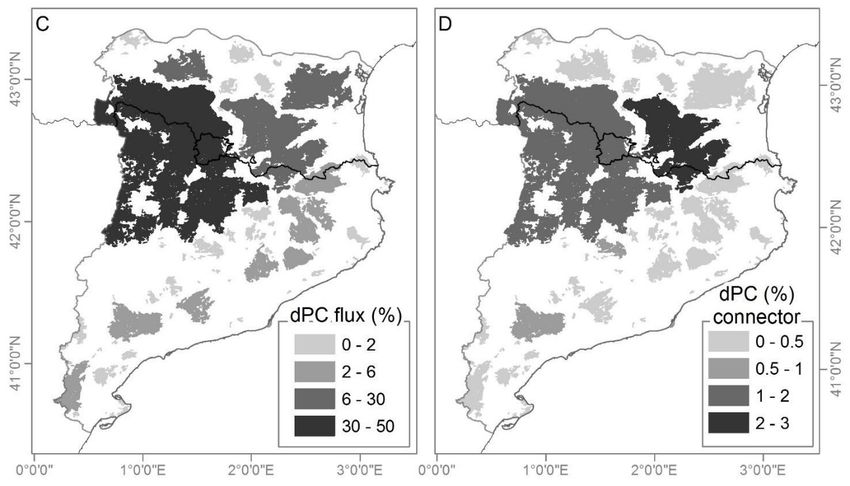
Sustainability 2020, 12, 5762                                                                         4 of 20

2. Study Area
       The area covered by this cross-border study comprises the entire territory of Catalonia,
the French side of the Eastern Pyrenees (made up of the regions of Haute-Garonne, Ariege, Aude,
and Pyrénées-Orientales), and the small state of Andorra (Figure 1), totaling an area of approximately
49,000 km2 . Although the average elevation of the area under study is not particularly high (over 75%
of it is below 1000 m), the territory extends to the Eastern Pyrenees, which reaches a maximum altitude
in the Pica d’Estats (3147 m). The great mountain range of the Pyrenees runs east to west along the
northern edge of the area.
       The study area has a notable variety of climates given the geographical shape and orientation of
the landforms: coastal Mediterranean, Mediterranean with a continental tendency, sub-Mediterranean,
Atlantic, and mountain. The vegetation of the area is thus characteristic of three distinct biogeographical
regions: predominantly Mediterranean, but also an abundance of Eurosiberian and, to a lesser extent,
Boreo-alpine vegetation [23]. This great variety in climate, vegetation, and altitude provides the
necessary conditions for a huge diversity of fauna. There is an abundance of Pyrenean chamois
(Rupicapra pyrenaica), roe deer (Capreolus capreolus), wild boar (Sus scrofa), hare (Lepus europaeus) and,
to a lesser extent, mouflon (Ovis orientalis) and red deer (Cervus elaphus), all potential prey for the wolf.
       Regarding land cover in the study area, the predominant types are forests (40%) and arable lands
(33%), followed by scrub and grassland (20%), while built-up areas occupy just 4% and pastures
3% [24–26]. Although pastures occupy a relatively low percentage of land in comparison with other
types of use, extensive stockbreeding mainly of horses and cattle, but also to a lesser extent of sheep and
goats, is particularly common in the Pyrenees. The areas occupied by forests, scrub, and grasslands,
which together comprise more than 50% of the terrain, are mostly located at higher altitudes, where most
of the protected areas of ecological and landscape value are also found. In total, more than 35% of the
study area comes under some type of environmental protection.
       From a demographic point of view, the area of study has a large human population imbalance
with 85% of the Catalan population living in coastal areas [27], more than half of which are in the
metropolitan area of Barcelona, where the density is between 1000 and 2000 inhabitants/km2 [28].
The Pyrenees are the least densely populated region of the study area with 30 inhabitants/km2 on the
Catalan side of the mountain range [28] and 100 inhabitants/km2 on the French side [29]. Andorra is
the most populated area in the Pyrenees, with 165 inhabitants/km2 [30].

3. Materials and Methods
     Conefor 2.6, a software based on ecological connectivity, was used to assess the landscape
connectivity for wolf habitat [31]. This software uses availability, quality, and effective connectivity
between habitat patches to develop a set of indicators that provide information on the probability
of species dispersal and the probabilistic and topological relationships established between habitat
fragments, according to graph theory [31,32].
     A patch-based graph of landscape is defined using two basic elements: the spatial distribution of
suitable habitat fragments (also called patches or nodes) and the set of connections (links) established
between the nodes. A component is a set of nodes interconnected either directly or indirectly via
stepping stones [33,34]. In this context, connectivity is conceived as the property of the landscape that
determines the amount of reachable habitat in that landscape (intrapatch connectivity), via connections
between different nodes (interpatch connectivity). Connectivity is often measured using a combination
of interpatch and intrapatch connectivity [31]. Different studies in Europe quantify the suitable
habitat for large mammals and then analyze the patch connectivity based on landscape graph-based
models [35] or using cost-path analysis techniques [36]. The specific steps and processes that were
carried out in this study are specified below.
Sustainability 2020, 12, 5762 5 of 20
3.1. Habitat Availability Map
A digital cartographic technique, known in Geographic Information System (GIS) language as
“weighted overlay”, was used to obtain the habitat availability map for the wolf. This technique
consists of superimposing the weighted variables that are considered to have the greatest influence
on the wolf habitat (Table 1). The method used for this calculation is commonly applied to analyze
both habitat availability [37–40] and movement of species through the landscape matrix [40–43].
The methodological process used is similar to developing a habitat suitability model based on
environmental parameters [44].
The following methodology was applied to achieve fragments of potential wolf habitat:
(i) computation of criteria weights using the Analytic Hierarchy Process (AHP), which has also
been widely incorporated into different GIS applications to analyze suitability [45,46]; and (ii) the
Ordered Weighted Averaging (OWA) method for producing suitability maps and running sensitivity
analyses [47].
The AHP converts these evaluations into numerical values (weights or priorities), which are used
to calculate a score for each alternative. A consistency index (CR) measures the extent to which the
decision-maker has been consistent in its responses. Based on [45], if the CR < 0.10, the pairwise
comparison matrix has an acceptable consistency and the weight values are valid and can be utilized.
Otherwise, if the CR ≥ 0.10, then the pairwise comparisons lack consistency and the matrix needs to be
adjusted and the element values modified.
The OWA operator was first introduced to address the problem of aggregating a set of criteria
functions to form an overall decision function [48]. OWA operators have been especially extensively
used in Multiple Criteria Decision Analysis (MCDA) to provide support in complex decision-making
situations, and they have notably been applied in GIS environments to produce land-use suitability
maps with applications in land-use planning and management, such as landslide susceptibility
mapping, wilderness mapping, ecological capability assessment, and so on. [49].
Cartographic analysis is known in GIS language as a “permeability matrix” or “friction map”,
used in this study to quantify the habitat available to the wolf throughout the area of study. This analysis
can be interpreted from a map depicting the cost or friction area, calculating the difficulty the wolf
has to move in space, and demonstrating the degree of suitability of the habitat for a certain species
(Figure 2A). This map differentiates between areas with a higher travel cost and those with the least
accumulative travel cost, representing the least and most favorable areas, respectively. By selecting the
most favorable locations, the most suitable areas for wolf settlement is obtained, constituting the wolf
habitat availability map.Sustainability 2020, 12, 5762 6 of 20
Table 1. Data source used for the elaboration of the wolf habitat suitability map.
State Layer Date Source Scale
Habitat typology 2005 DTES (Department of Territory and Sustainability) and University of Barcelona 1:50,000
River network 2004 Catalan Water Agency (ACA) 1:50,000
Rail network 2007 DTES 1:5000
Spain Road network 2013 DTES 1:5000
Nature Network 2000 2013 DTES 1:50,000
Urban areas 2005 Extracted by habitat typology layer 1:50,000
Digital Elevation Model 2014 Catalan Institute of Cartography and Geology (ICGC) 15 m resolution
Habitat typology (CORINE Land Cover) 2006 European Environment Agency (EEA) 1:100,000
River network 2014 Open Street Map (OSM) -
Rail network 2014 OSM -
Road network 2014 OSM -
France
Nature Network 2000 2011 EEA 1:100,000
Natural Regional - Ministry of Ecology, Sustainable Development and Energy -
Urban areas 2006 Extracted by habitat typology layer 1:100,000
Digital Elevation Model 2003 EEA 30 m resolution
Habitat typology 2012 Institute of Andorran Studies 1:25,000
River network 1995 Institute of Andorran Studies 1:5000
Road network 1995 Department of Environment 1:5000
Andorra
Natural Parks 2013 Department of Environment 1:25,000
Urban areas 2012 Extracted by habitat typology layer 1:25,000
Digital Elevation Model 1995 Department of Environment 5 m resolutionThe territory used by the packs is considered as the space required for lone wolves to form stable
populations or packs if the requisite conditions for reproduction are met. Recent studies have shown
that for Iberian wolves this area is on average around 200 km2 [52]. The packs of Italian wolves that
have recently arrived in Mercantour similarly use an area of approximately 200 km2 to this end [55].
In line with these data, only patches larger than 200 km2 were selected to analyze the ecological
Sustainability 2020, 12, 5762 7 of 20
connectivity of the landscape by means of a set of indices presented in the following section.
Figure 2. (A) Wolf friction map or degree of suitability for wolf habitat. (B) Optimal areas for wolf
Figure 2. (A) Wolf friction map or degree of suitability for wolf habitat. (B) Optimal areas for wolf
habitat classified according to size: only fragments above 200 km2 are suitable for hosting stable packs
habitat classified according to size: only fragments above 200 km2 are suitable for hosting stable packs
of wolf populations. The red squares indicate the presence of wolves at some time since 2000. Areas
of wolf populations. The red squares indicate the presence of wolves at some time since 2000. Areas
with permanent wolf presence: 1—Alt Ripollès; 2—Alta Cerdanya. The most suitable fragments for
with permanent wolf presence: 1—Alt Ripollès; 2—Alta Cerdanya. The most suitable fragments for
wolf settlement (Figure 2B) are distributed along the main mountain ranges of the area of study and
occupy almost one-third of the entire area.
Suitability Map Based on Wolf Ecology Criteria
Different published information [4,9,50–58] was considered to establish the ecological criteria and
to create the wolf habitat suitability map. These studies consider some variables as key factors of wolf
presence, such as roads, human settlements, altitude, protected areas, and type of habitats. However,
no studies were found that deal with all the factors together to assess the influence of each variable
for habitat suitability for the wolf. This paper, however, considers all the relevant environmental
variables that could influence wolf survival according to the literature consulted: (i) type of habitat;
(ii) proximity to watercourses; distances from (iii) urban areas, (iv) roads, and (v) railways; (vi) altitude;
and (vii) protected natural areas.
Following processing using a combination of GIS tools (buffer, clip, merge, Euclidean distance,
among others), the vector layers were rasterized using a pixel resolution of 30 m2 . The variables were
then duly reclassified using a certain cost value of suitability for the wolf (Table 2). The values allotted
to each variable and the weighted overlay of the layers were based on data on wolf habitats published
in scientific journals. This methodological process based on the literature is frequently used as the
basis for modelling connectivity for conservation initiatives [40]. Notably, however, the method used
for the weighted overlapping of layers produces a few problems and limitations, among which the
interpolation of the data should be highlighted [59].
One of the main variables that determine whether the wolf will settle in an area is the availability
of prey, which depends largely on land cover, habitat type, and human activities, such as hunting
management and grazing. The wolf adapts its diet to the environmental conditions of the territory in
which it lives and the availability of prey, feeding on different kinds of prey depending on availability,
with the composition of these species varying among the study areas. According to Zlatanova et al. [60],
in Scandinavia the wolf feeds on wild ungulates such as elk (Alces alces) and reindeer (Rangifer tarandus);Sustainability 2020, 12, 5762 8 of 20
on red deer, roe deer, and wild boar in Central Europe; and usually on wild boar and roe deer in
Southern Europe. If there is a shortage of wild ungulates, however, the wolf will feed on livestock or
even plant food, smaller prey, and garbage.
Table 2. Variables used in the wolf friction map. The permanent watercourses were selected for rivers
and only the basic road network, consisting of highways, two-lane roads, and basic regional roads,
were considered for roads.
Protected Natural Areas Proximity to Urban Areas Proximity to Roads Proximity to Railway Lines
Classification Cost Value km Cost Value km Cost Value km Cost Value
Category I–II (UICN) 1 0–0.5 10 0–0.5 10 0–0.25 10
Category III–IV 2 0.5–3 9 0.5–2 9 0–2 6
Category V–VI 3 3–6 7 2–4 8 2–4 4
Non-protected area 7 6–10 5 4–8 6 >4 2
10–12 3 8–12 2
>12 1 >12 1
Proximity to
Habitat Type Altitude (m)
Water Sources
Classification Cost Value km Cost Value Threshold Cost Value
Small bodies of fresh water 3 0–0.10 10 0–500 6
Bodies of saline water 9 0.10–3 1 500–1000 2
Canals, reservoirs, and dams 9 3–5 2 1000–2000 1
Sandy and silty coastal plains 7 5–12 3 >2000 3
Saline scrublands and grasslands 7 >12 5
Beaches 9
Littoral cliffs 9
Cliffs and rocky inlands 2
Scrublands 2
Grasslands and crops 2
Forests 1
Flooded habitats 6
Peat lands 2
Rocky screes 8
Glaciers and areas with
5
permanent snow
Woody and arable crops 3
Tree plantations 3
Urban parks and gardens 10
Cities, towns, and industrial areas 10
Abandoned fields and
5
ruderal areas
Logged and burned areas 9
Studies on wolf populations in human landscapes have determined that the density of wolves
is directly related to the density of prey in the wild [58], and it is here that forest areas are especially
valuable. Territory bordering on cropland is also sought by the wolf given that it is home to abundant
prey such as wild boar, the numbers of which are currently increasing. Mountain crags are also used
by wolves to hunt wild ungulates, where they establish their dens in natural holes in the ground [55].
Hence, in this study the land cover variable was given four times the weight of the other variables
given that it is considered to exert a greater influence on habitat availability. This means that land
cover was weighted 40%, while the other variables (Table 2) were each weighted 10%.
Forest cover was considered as the most favorable for wolf habitat, followed by scrub, moorland,
meadows, and pastures, and to a lesser extent cropland (Table 2). Despite some studies determining that
wolves avoid agricultural lands for breeding [61], there is evidence of stable packs of wolf populations in
a northern-central Spanish agricultural area with a high human population density [62–64]. The highest
friction cost value was assigned to built-up areas (Table 2).
Rivers do not constitute a barrier for the wolf as it can cross them with relative ease, depending
on the flow and strength of the current, sometimes even entering them in pursuit of prey. The wolf
only avoids extremely large bodies of water or deserts for both habitation and movements for
dispersal [64,65]. Considering its daily need for water, especially during the denning period when
breeding, it can be assumed not to stray too far from this resource.Sustainability 2020, 12, 5762 9 of 20
Studies on the presence of the wolf in Galicia have also determined altitude to be a key factor
in the distribution of this species [58], the probability of wolf presence in the territory progressively
increasing with altitude. The wolf tends to avoid lower areas and medium-low altitudes where there
are human settlements and human activities taking place, both of which decrease with increasing
altitude [37]. According to Llaneza et al. [58], the maximum probability of wolf presence is located
at an altitude of between 1000 and 2000 m, above which the likelihood of finding wolves once again
decreases. This consideration was considered when allocating the friction cost values at different
intervals of the altitude variable (Table 2).
Although it is not a very shy animal, the wolf endeavors to avoid noisy and frequented places,
such as the great urban areas and transport infrastructures [53,58,61,66]. The presence of inhabited
areas is one of the main variables that determines wolf presence in a territory [67]. Studies conducted
in the north-west of the Iberian Peninsula verify that wolf presence increases with decreased housing
and population density [53,58]. The probability of wolf presence in humanized landscapes increases
as the density of roads per square kilometer decreases and the distance from the main road network
increases. This has been evidenced in the Iberian Peninsula [53,57,58], as well as in some places in
Europe [61,68,69] and in the United States [50]. In fact, more than 50% of wolf casualties result from
impact on roads [51,54]. According to Rodríguez-Freire and Crecente-Maseda [56], highway AP-9 may
have divided the existing population of wolves in the north-west of the Iberian Peninsula into two
groups all along the road.
In a study of wolf populations in the north-west of the Iberian Peninsula, Vilà et al. [51] determine
their daily movements to range between 10 km and 12 km. Hence, a threshold of 12 km was used for
the friction cost value in relation to distance from waterbodies, urban areas, and roads. The use of
distance thresholds for certain landscape elements to assess their impact on the distribution of species
is common in this type of research [41,42]. These studies also analyze different landscape elements and
weigh them to assess the habitat suitability of species.
Protected natural areas were weighted positively. Human activities that can disturb wolf presence,
such as hunting and access for motor-driven vehicles, are forbidden or regulated in protected areas.
To this effect, the different categories of the IUCN (International Union for Conservation of Nature)
classification were considered (Appendix A). The more protected the area, the more positively the
variable was weighted (Table 2). Nevertheless, in the study area, most of the natural protected areas
correspond to categories V and VI of the IUCN classification.
Using the suitability map, places of less value on the map were selected (with pixel values < 3),
thus producing the availability map or optimal areas for the wolf. The areas where the wolf could
form stable packs were then differentiated from those where it could only make sporadic incursions.
The territory used by the packs is considered as the space required for lone wolves to form stable
populations or packs if the requisite conditions for reproduction are met. Recent studies have shown
that for Iberian wolves this area is on average around 200 km2 [52]. The packs of Italian wolves that
have recently arrived in Mercantour similarly use an area of approximately 200 km2 to this end [55].
In line with these data, only patches larger than 200 km2 were selected to analyze the ecological
connectivity of the landscape by means of a set of indices presented in the following section.
All the cartographic information was processed using the ESRI ArcMap program. A UTM
(Universal Transverse Mercator) map projection was employed to work on the maps using the reference
system ETRS89 (European Terrestrial Reference System 1989), UTM zone 31N. The original scale of
the different information layers used for this analysis should be considered since this determines the
degree of detail in the resulting mapping. To this effect, the type of habitat map in France was made on
a large-scale (1:100,000), while the habitat map in Catalonia was on a scale of 1:50,000, and the habitat
map in Andorra was on a scale of 1:25,000 (Table 1).Sustainability 2020, 12, 5762 10 of 20
3.2. Assessing Habitat Availability and Connectivity
Conefor, a management support tool that quantifies the importance of each habitat by fragmenting,
functionally maintaining, or increasing landscape connectivity, was used to assess the landscape
connectivity of the wolf. The probability of connectivity (PC) indicator, one of the most recommended
indexes for planning and decision-making, also used for assessing the state of connectivity of
different species [70,71], was employed. This index quantifies functional connectivity between a set
of interconnected nodes and is obtained by weighting the attributes given to each habitat fragment
(in this case, the surface area occupied by each fragment) and the dispersal probability of each node
with the remaining nodes. It is given by the following expression [72]:
Pn Pn ∗
i=1 j=1 ai a j pij
PC = (1)
A2L
where ai and a j are the area of the habitat patches i and j, n is the number of habitat patches in the
landscape, AL is the total landscape area (habitat and non-habitat patches), and pij is the product
probability of an animal moving directly from patch i to j over the shortest path. p∗ij is the maximum
product probability of all possible paths between patches i and j (including single-step paths).
The contribution to overall habitat availability and connectivity is calculated by the relative
ranking of each patch:
PC − PC0
dPCk (%) = (2)
PC
where dPCk is the importance of node k to overall habitat availability in the landscape. PC0 is the PC
value after removing k from the analysis. The dPCk [73] can be divided into three fractions according to
the different ways each path can contribute to habitat connectivity and availability in the landscape:
dPCk (%) = dPCintrak + dPC f luxk + dPCconnectork (3)
where dPCintrak corresponds to the available habitat area provided by patch k in terms of intrapatch
connectivity. The topological relationships (the position of each node within the landscape network)
between each patch do not affect the calculation of this metric; only local features (area) do. dPCfluxk is
the flux through connections of patch k to or from all the other patches in the graph structure when k is
the start or end node of that flux. In this case, the local characteristics of the patch and its position
within the landscape network affect the computation of this fraction and a patch with a higher attribute
value produces more flux if the rest of the factors are equal. dPCconnectork is the contribution of k to
the connectivity between other habitat patches as a connecting element (or stepping stone) between
them. The calculation of this metric only depends on the topological relationships; any other attribute
considered does not affect this fraction.
Corridors or links established between nodes are determined by the wolf’s ability to move from
one node to another through an unfavorable area. In this study, it was considered that there is a 50%
probability of the species moving between different habitat fragments if the distance between them in a
straight line was 75 km or less. The same dispersal distance was established for both males and females,
although males tend to disperse at higher rates than females [74,75]. Saura and Pascual-Hortal [72]
recommend a probability value of 0.5 as the distance corresponding to the median dispersal distance
of the species under analysis.
The threshold distance of 75 km is equal to the average annual number of kilometers travelled
by the wolf on its journey from the French Alps to the Eastern Pyrenees [17]. It is also equivalent to
the Euclidean distance of some wolves’ intrusions from the Cadí-Moixeró (the place most frequented
by wolves in Catalonia) to outlying areas such as the regions of Moianès and Osona [14], or more
recently the Gavarres Massif (Figure 2B). The fact that wolves adapt well to different environmentalSustainability 2020, 12, 5762 11 of 20
conditions [3,62,76] means that they can travel great distances through fairly unfavorable habitat
(as demonstrated by the dispersal of the Italian wolf from the central Apennines to the Eastern Pyrenees).
4. Results
One-third of the study area can be considered as potential habitat for the wolf, and more than
90% of this space is suitable for hosting stable packs. The most suitable areas are the main mountain
ranges and forests, coinciding with those inhabited by humans (Figure 2A). Specifically, these areas are
located in the area of the High Catalan Pyrenees and the Cadí Massif on the Spanish side; and the
Regional Natural Park of the Catalan Pyrenees, the Regional Natural Park of the Ariège Pyrenees,
and the Corbières Massif on the French side.
Various scenarios were simulated to attribute different weights to the layers and to estimate the
sensitivity of different schemes (Table 3). The seven variables were weighted differently according
to three scenarios, supplying distinct availability maps with a diverse number of pixels with
high suitability (Sustainability 2020, 12, 5762 12 of 20
in the countryside studied (7950 km2 ) and with a dPC value of 75.3% (Table 4). This fragment also
shows high values of intrapatch connectivity or dPCintra (24.3%), and of dPCflux (49.6%). Secondly,
Node 2 is in the Alta Cerdanya, Alt Ripollès, and the Regional Natural Park of the Catalan Pyrenees,
occupying 2500 km2 and showing the highest contribution to connectivity among other habitat patches
as a connecting element or stepping stone (dPCconnector = 2.8%). This node also contributes through
connections from Node 2 to all the other patches in the graph structure or from all the other patches to
thisSustainability
node (dPCflux2020, 12,= 26.16%).
x FOR PEER REVIEW 12 of 20
Figure
Figure Importance
3. 3. Importanceofofwolf
wolfhabitat
habitatfragments
fragments according
according toto the
thedPC
dPC(A)(A)probability
probabilityofofconnectivity
connectivity
andandthethe
three fractions of dPC: dPCintra (B) the available habitat area provided by a patch
three fractions of dPC: dPCintra (B) the available habitat area provided by a patch itself itself in terms
in
of intrapatch connectivity;
terms of intrapatch dPCfluxdPCflux
connectivity; (C) the flux through
(C) the connections
flux through of a patch
connections of atopatch
or from
to orallfrom
the other
all
patches in the
the other graphin
patches structure when
the graph this patch
structure whenis this
the start
patchorisend
the node of end
start or that node
flux; and dPCconnector
of that flux; and
(D)dPCconnector (D) the
the connectivity connectivity
between between
other habitat other habitat
patches patches aselement
as a connecting a connecting elementstone
or stepping or stepping
between
stoneNodes
them). > 200
between them). 2 are numbered
kmNodes are numbered
> 200 km2 from 1 to 12. from 1 to 12.
5. Discussion
5.1. Large Expanse of Land Available for Movement and Settlement
The availability of a habitat and good connectivity between fragments make the presence of the
wolf possible over a large part of Catalonia and the northern side of the French Pyrenees. However,
Mech [77] shows that some models of area prediction for recovering the wolf fail. Thus, the patches
suitable for the species can be understood as an indication of where wolves will probably settle firstSustainability 2020, 12, 5762 13 of 20
Table 4. Importance of wolf habitat fragments > 200 km2 according to the dPC (probability of
connectivity) and the three fractions of dPC: dPCintra (the available habitat area provided by a patch
itself in terms of intrapatch connectivity); dPCflux (the flux through connections of a patch to or from
all the other patches in the graph structure when this patch is the start or end node of that flux);
and dPCconnector (the connectivity between other habitat patches as a connecting element or stepping
stone between them).
Node dPC dPCintra dPCflux dPCconnect km2
1 75.32 24.36 49.67 1.29 7951.60
2 31.38 2.42 26.15 2.81 2505.50
3 14.24 0.59 13.64 0.01 1234.08
4 6.80 0.15 5.67 0.98 625.46
5 6.64 0.12 6.51 0.01 562.31
6 6.22 0.10 5.93 0.20 502.42
7 5.73 0.09 5.49 0.16 470.54
8 3.45 0.03 2.97 0.45 291.75
9 3.37 0.07 3.28 0.02 412.76
10 3.02 0.03 2.99 0.00 265.75
11 2.72 0.02 2.68 0.02 234.41
12 2.65 0.02 2.50 0.14 209.84
The rest of the nodes showing significant values are located on the edge of the two principal
patches (Nodes 1 and 2), also especially contributing across the dPCflux which, on the one hand, takes
the topological positions of the nodes within the entire network into account and, on the other hand,
considers the attribute of the node (area). On the French side, the Corbières (Node 3) and an isolated
fragment of the Pyrenean Ariège (Node 5) stand out. In Catalonia, secondary nodes can be found in
the Alta Garrotxa (Node 6), the Transversal Mountain Range (Nodes 7 and 12), and the Pre-Coastal
Mountain Range. In this mountain range, the Montsant–Prades Mountains (Node 4), the Ports de
Beseit (Node 9), the Montmell–Ancosa sector (Node 8), Sant Llorenç del Munt (Node 10), and Montseny
(Node 11) stand out.
5. Discussion
5.1. Large Expanse of Land Available for Movement and Settlement
The availability of a habitat and good connectivity between fragments make the presence of the
wolf possible over a large part of Catalonia and the northern side of the French Pyrenees. However,
Mech [77] shows that some models of area prediction for recovering the wolf fail. Thus, the patches
suitable for the species can be understood as an indication of where wolves will probably settle first
rather than the places where they will actually become established in the medium and long term.
The state of ecological connectivity between the patches studied reveals that the area is a single
component where wolves can move anywhere. Each node is connected to the others either directly or
via other nodes (stepping stones) given that in all cases the distance to another node is less than the
considered dispersal distance of 75 km. Establishing a specific dispersal distance has proven difficult
since wolves can successfully disperse through hostile, unsuitable areas [65,78] for various lengths of
time and distance [12,79]. In Europe, some studies present dispersal rates similar to the one chosen
in this study, as is the case with Finnish wolves who showed a dispersal distance of 98.5 km [80].
However, this number may be much higher, estimated at between 250 and about 400 km [81–83],
and even reaching 800 km in the movements of the population of German wolves to Poland [12].
Ciucci et al. [83] determine the Italian grey wolf straight line dispersal distance (from the Northern
Apennines to the Alps) as 240 km. Similar data were presented by Ražen et al. [84], who set the
straight line dispersal distance between the Dinaric-Balkan and Alpine grey wolf populations at 230 km.
Exceptionally, Blanco and Cortés [63] determine a low range of 31.5 km as the dispersal distance for
male grey wolves in the north-central region of Spain.Sustainability 2020, 12, 5762 14 of 20
Other studies show similar dispersal distances for male grey wolves in North America.
Ballard et al. [85] studied the dispersal of the wolf in Southcentral Alaska, determining the dispersal
distance for males as 84 km; Gese and Mech [86] determined the male grey wolf mean dispersal
distance in north-east Minnesota as 88 km; Wydeven et al. [87] fixed the mean distance of 65 km for
the dispersal of wolves in Wisconsin; and Jimenez et al. [75] recently set male grey wolves’ dispersal
distance in the Rocky Mountains (North West America) at 98.1 km.
In the area of study, the fragments that contribute most to habitat availability (via intrapatch
or interpatch connectivity) are in the Pyrenees and the Pre-Pyrenees. The samples collected and
observations of the species verify that the places most visited by the wolf in Catalonia during the
period in question was the areas Cadí Massif, Alt Ripollès, and Alta Cerdanya, while in France it
was the Eastern Pyrenees (Figure 1). These areas are not only the largest and best connected with
the rest according to the results obtained (Figures 2 and 3), but they also have a wide variety of
potential prey for the wolf, such as the hare, the wild boar, the roe deer, the mouflon, and the Pyrenean
chamois [14,15,19].
5.2. The Pyrenees, a Strategic Location for Wolf Conservation in Europe
Conservation of regional habitat connectivity has the potential to facilitate the recovery of the wolf,
which is currently recolonizing portions of its historic range of distribution. The geographical situation
of Catalonia makes it a suitable meeting point between the Iberian Peninsula’s own wolf population
and the population originating in the Italian Apennines. The differences between the two populations
make wolf colonization of the Pyrenees a conservation goal itself, with the aim of increasing the gene
flow between populations. A new established population in the Pyrenees could lead to more genetic
exchange between the Iberian population and those in the rest of Europe, which would be a further
step in re-establishing natural gene flow. Increasing the number of habitat fragments suitable for the
wolf all across Europe to act as stepping stones would be a good strategy to conserve regional habitat
connectivity and to maximize species protection at a minimum cost, in addition to being a step further
in re-establishing natural gene flow between the wolf populations in Spain and the rest of Europe.
In this regard, it would be of great interest to quantify how the Pyrenees is contributing to the
global landscape connectivity for wolves in Europe. A study similar to the present one could be
performed to determine the dPCconnector, which is the contribution of each patch to the connectivity
between other habitat patches as a connecting element or stepping stone between them [31].
5.3. Management, the Key to Maximize Conservation and Minimize Conflicts
To the north of the river Duero the wolf is a hunted species, meaning that individuals in
these populations can be indiscriminately killed. On the other side of the Pyrenees, however,
the environmental conservation and recovery policies undertaken in much of Europe, coupled with
threatened species protection, has made it possible to promote a slow but steady recovery in certain
areas of the continent, especially in Italy, Switzerland, and Eastern and Central France [88]. This may
explain why the wolf coming from Italy arrived in the Pyrenees before the Iberian one. Nonetheless,
the lack of legislation in Spain for protecting the wolf in the Pyrenees and the current hunting plan for
wolves in France may have led to the drastic decrease in individuals detected prior to 2011. Recent
hunting activity in France has reduced the flux of lone wolves, resulting in the Madres Massif being
recently re-classified as an area of temporary wolf presence given that its presence has not been able to
be confirmed during the last two winters [18]. The reduction of flux from France impedes new arrivals
in the Eastern Pyrenees coming from the European continent. However, the wolf’s high reproductive
potential and long-distance dispersal ability are crucial for its resilience and quick recovery in areas
where they have been exterminated by indiscriminate hunting by humans [78,89].
Sooner or later wolves will become established in the Pyrenees, so it is important to know where
they will potentially settle to be able to foresee and mitigate potential human–wolf conflicts. The most
suitable areas for the wolf revealed by this analysis are those where future conflicts with livestockSustainability 2020, 12, 5762 15 of 20
owners are expected. Hunting tourism will also be a source of conflict with ecologists, with the wolf
hunted in accordance with the laws of each European country.
Mech [90] evinces various practices in different European countries (Germany, France, Sweden,
or Finland) that flaunt legislation and go against the expansion of the species, including poaching
and hunting. Nevertheless, culling of the wolf population by means of drives has failed in its goal of
reducing depredations on livestock in Spain [91]. It is well known that uncontrolled dogs could be
responsible for some of the attacks on livestock. Echegaray and Vilà [10] found that most of the wolf
feces they analyzed contained the remains of wild prey, whereas the dog feces they examined mainly
contained the remains of domestic animals. Imbert et al. [92] also indicates that wolves in Liguria
consume mainly wild ungulates and, to a lesser extent, livestock. In the same region, Torretta et al. [93]
show that the species most consumed by wolves are wild boar and roe deer. Llaneza and López-Bao [94]
show how in the north-west of Spain changes in agricultural and environmental policies over the
last three decades have shifted the wolf’s diet, 95% of which was previously based on anthropogenic
food sources.
Despite the numerous scientific arguments, the recovery of wolf populations in rural areas is
not welcomed. People living far from wolf territories have more positive attitudes towards wolf
conservation than those living within or close to wolf territories [95]. Conflicts between policies and
biodiversity conservation are not always easy to manage. The interests of the agents involved are in
conflict and it is difficult to design management policies that satisfy both visions. Therefore, it is hugely
important to integrate policies into biodiversity conservation to anticipate future wolf–human conflicts.
Mech [90] indicates the need to modify the Bern Convention (Council of Europe 82/72/CEE) and the
European Habitat Directive (Council Directive 92/43/EEC), enacted to re-establish wolf populations,
according to local situations, so that wolves are able to live alongside humans with only minimal conflict.
To this effect, the Finnish literature could be a reference for integrating efficient conservation policies.
Karlsson and Sjöström [95] suggest that surveys of human perception towards wolf conservation
should be done in territories where conservation and management initiatives are expected to be carried
out. However, after studying citizens’ perceptions using surveys, Bisi et al. [96] state that people living
in areas where wolves occur feel that neither legislative bodies nor conservationists listen to their
opinions. They report that their requests have not been heard, while concessions to these requests
would create a universally supported policy or would at least increase tolerance of wolves.
6. Conclusions
This paper presents a method for identifying and assessing the availability and ecological
connectivity of wolf habitat in the Eastern Pyrenees. It is a procedure that should be implemented
from the Italian Peninsula to the Iberian Peninsula, via the French Mediterranean, to be able to analyze
the capacity of the region to accommodate wolf dispersal flows in the coming years.
Protection of the species in Catalonia and France will play a key role if the flow of lone wolves
reaches the levels of previous years. Wolf settlement and dispersal in certain parts of the area of study
could consequently become a reality in the following decades. In the medium to long term, protection
of the species may lead to the settlement of stable wolf packs in the Pyrenees, from where they would
disperse into better connected adjacent areas (Pre-Pyrenees) and make occasional incursions to the
better connected points (central Catalonia and the Coastal Mountain Range). The environmental
conditions are even favorable enough for some individuals to disperse through the interior of the
Iberian Peninsula via the Pyrenees and the Coastal Mountain Range. In the long run, the Pyrenees
could become a meeting area between the wolves of the Iberian Peninsula and the populations in the
Alps and the Apennines.
Author Contributions: Conceptualization, C.G.-L. and D.V.; methodology, C.G.-L.; D.V.; J.P. and F.X.R.-M.;
software, C.G.-L. and D.V.; validation, C.G.-L. and D.V.; formal analysis, C.G.-L. and D.V.; investigation, C.G.-L.;
resources, J.P.; data curation, C.G.-L.; writing—original draft preparation, C.G.-L.; D.V.; J.P. and F.X.R.-M.;
writing—review and editing, C.G.-L. and D.V.; visualization, C.G.-L.; supervision, D.V.; J.P. and F.X.R.-M.; projectSustainability 2020, 12, 5762 16 of 20
administration, J.P.; funding acquisition, J.P. All authors have read and agreed to the published version of
the manuscript.
Funding: This research received no external funding.
Conflicts of Interest: The authors declare no conflict of interest.
Appendix A
Table A1. Protected area categories according to the International Union for the Conservation of Nature.
Categories Main Features
Protected areas that are strictly set aside to protect biodiversity
and possibly geological/geomorphological features, where
Ia. Strict Nature Reserve
human visitation, use, and impacts are strictly controlled and
limited to ensure protection of the conservation values.
Protected areas that are usually largely unmodified or slightly
Ib. Wilderness Area modified, retaining their natural character and influence,
without permanent or significant human habitation.
Large natural or near natural areas set aside to protect large-scale
ecological processes. They also provide a basis for
II. National Park
environmentally and culturally compatible spiritual, scientific,
educational, and recreational activities.
Areas set aside to protect a specific natural monument. They are
III. Natural Monument or Feature generally quite small protected areas and often have high
visitor value.
Protected areas aimed at protecting particular species or habitats,
and their management reflects this priority. Regular and active
IV. Habitat/Species Management Area
interventions are needed, but this is not a requirement of
the category.
A protected area where the interaction of people and nature over
V. Protected Landscapes/Seascape time has produced an area with a distinct character of significant
ecological, biological, cultural, and scenic value.
Protected areas that conserve ecosystems and habitats, together
with associated cultural values and traditional natural resource
VI. Protected area with sustainable uses of
management systems. Low-level non-industrial use of natural
natural resources
resources compatible with nature conservation is seen as one of
the main aims of the area.
IUCN protected area management categories classify protected areas according to their
management objectives. The categories are recognized by international bodies such as the United
Nations and by many national governments as the global standard for defining and recording protected
areas and as such are increasingly being incorporated into government legislation.
References
1. Hoffmann, M.; Hilton-Taylor, C.; Angulo, A.; Böhm, M.; Brooks, T.M.; Butchart, S.H.M.; Carpenter, K.E.;
Chanson, J.; Collen, B.; Cox, N.A.; et al. The Impact of Conservation on the Status of the World’s Vertebrates.
Science 2010, 330, 1503–1509. [CrossRef]
2. Butchart, S.H.M.; Walpole, M.; Collen, B.; Van Strien, A.; Scharlemann, J.P.W.; Almond, R.E.A.; Baillie, J.E.M.;
Bomhard, B.; Brown, C.; Bruno, J.; et al. Global Biodiversity: Indicators of Recent Declines. Science 2010, 328,
1164–1168. [CrossRef] [PubMed]
3. Mech, L.D. The Challenge and Opportunity of Recovering Wolf Populations. Conserv. Biol. 1995, 9, 270–278.
[CrossRef]
4. Hearn, R.; Balzaretti, R.; Watkins, C. The Wolf in the Landscape: Antonio Cesena and Attitudes to Wolves in
Sixteenth-Century Liguria. Rural. Hist. 2015, 26, 1–16. [CrossRef]Sustainability 2020, 12, 5762 17 of 20
5. Dressel, S.; Sandström, C.; Ericsson, G. A meta-analysis of studies on attitudes toward bears and wolves
across Europe 1976-2012. Conserv. Biol. 2014, 29, 565–574. [CrossRef] [PubMed]
6. Núñez-Quirós, P.; García-Lavandera, R.; Llaneza, L. Análisis de la distribución histórica del lobo (Canis lupus)
en Galícia: 1850, 1960 y 2003. Ecología 2007, 21, 195–206.
7. de Beaufort, F. Le loup en France: Éléments D’écologie Historique. In Encyclopédie des Carnivores de France:
Espèces Sauvages ou Errantes Indigènes ou Introduites en Métropole et Dans Les DOM-TOM; Société Française
d’Etude et de Protection des Mammifères: Paris, France, 1987; Volume 1.
8. Manent, A. El llop a Catalunya: Memòria, Llegenda i Història; Pagès Editors: Lleida, Spain, 2004.
9. Hayes, C.T.; Martínez-Garcia, A.; Hasenfratz, A.P.; Jaccard, S.; Hodell, D.A.; Sigman, D.; Haug, G.H.;
Anderson, R.F. Recovery of large carnivores in Europe’s modern human-dominated landscapes. Science 2014,
346, 1517–1519. [CrossRef]
10. Gortázar, C.; Herrero, J.; Villafuerte, R.; Marco, J. Historical examination of the status of large mammals in
Aragon, Spain. Mammalia 2000, 64, 411–422. [CrossRef]
11. Echegaray, J.; Vilà, C. Noninvasive monitoring of wolves at the edge of their distribution and the cost of their
conservation. Anim. Conserv. 2010, 13, 157–161. [CrossRef]
12. Andersen, L.W.; Harms, V.; Caniglia, R.; Czarnomska, S.; Fabbri, E.; J˛edrzejewska, B.; Kluth, G.; Madsen, A.B.;
Nowak, C.; Pertoldi, C.; et al. Long-distance dispersal of a wolf, Canis lupus, in northwestern Europe.
Mammal Res. 2015, 60, 163–168. [CrossRef]
13. Bataille, A.; Briandet, P.E.; Chenesseau, D.; Duchamp, C.; Goujou, G.; Gallais, R.; Jean, N.; Leonard, Y.;
Schwoerer, M.L.; Steinmetz, J. Bilan du suivi hivernal 2016/2017. Bull. Loup Réseau 2017, 36, 18–25.
14. Lampreave, G.; Ruiz-Olmo, J.; Garcia-Petit, J.; López, J.M.; Bataille, A.; Sastre, N.; Francino, O.; Ramírez, O.
El lobo vuelve a cataluña: Historia del regreso y medidas de conservación. Quercus 2011, 302, 16–25.
15. Bataille, A.; Lampreave, G.; Duchamp, C. Les Pyrénées: Toujours pas de meute mais 2 nouvelles ZPP.
Bull. Loup Réseau 2015, 33, 25–28.
16. Valière, N.; Fumagalli, L.; Gielly, L.; Miquel, C.; Lequette, B.; Poulle, M.-L.; Weber, J.-M.; Arlettaz, R.;
Taberlet, P. Long-distance wolf recolonization of France and Switzerland inferred from non-invasive genetic
sampling over a period of 10 years. Anim. Conserv. 2003, 6, 83–92. [CrossRef]
17. Gonzàlez-Prat, F. El retorn del llop (Canis lupus, L. 1758) als Pirineus. (Reflexions sobre conservació de la
natura i el món pastorívol a la muntanya). Ann. Cent. d’Estudis Comarc. Ripollès 2002, 2000, 301–312.
18. Bataille, A. Congrès international en Espagne. Bull. Loup Réseau 2017, 36, 29–31.
19. Palazón, S. The Importance of Reintroducing Large Carnivores: The Brown Bear in the Pyrenees. In Advances
in Global Change Research; Springer Science and Business Media LLC: Berlin/Heidelberg, Germany, 2017;
Volume 62, pp. 231–249.
20. Fourli, M. Compensation for Damage Caused by Bears and Wolves in the European Union; DG XI European
Comunities: Luxemburg, 1999.
21. Fischer, J.; Lindenmayer, D.B. Landscape modification and habitat fragmentation: A synthesis.
Glob. Ecol. Biogeogr. 2007, 16, 265–280. [CrossRef]
22. Baranyi, G.; Saura, S.; Podani, J.; Jordán, F. Contribution of habitat patches to network connectivity:
Redundancy and uniqueness of topological indices. Ecol. Indic. 2011, 11, 1301–1310. [CrossRef]
23. Bolòs, O.; Vigo, J. Flora dels Països Catalans; Editorial Barcino: Barcelona, Spain, 1984–2001; Volume 4.
24. Departament de Territori y Sostenibilitat (DTOS) & University of Barcelona (UB). Cartografía de los Hábitats en
Cataluña 1:50.000, versión 2; Generalitat de Catalunya (GENCAT): Barcelona, Spain, 2008–2012.
25. Carreras, J.; Carrillo, E.; Ferré, A.; Perez-Haase, A.; Ninot, J.M.; Caritg, R. Mapa dels Hàbitats d’Andorra 2012 a
escala 1:25.000; Centre d’Estudis de la Neu i de la Muntanya d’Andorra de l’Institut d’Estudis Andorrans:
Andorra la Vella, Andorra, 2013.
26. European Topic Centre for Spatial Information and Analysis (ETC/SIA). Corine Land Cover 2006 Raster
Data. Raster Data on Land Cover for the CLC2006 Inventory, version 17; 100 Metros de Resolución; European
Environment Agency (EEA): København, Denmark, 2013.
27. Nel·lo, O. Ordenar el Territorio, el caso de Barcelona y Cataluña; Tirant Humanidades: Valencia, Spain, 2012.
28. Institut d’estadística de Catalunya (IDESCAT). Available online: www.idescat.cat (accessed on 5 June 2020).
29. Institutnational de la statistique et des études économiques (INSEE). Available online: www.insee.fr
(accessed on 5 June 2020).You can also read