TI-6AL-4V SELECTIVE LASER MELTING - A NOVEL PHYSICS-BASED AND DATA-SUPPORTED MICROSTRUCTURE MODEL FOR PART-SCALE SIMULATION OF
←
→
Page content transcription
If your browser does not render page correctly, please read the page content below
A N OVEL P HYSICS -BASED AND DATA -S UPPORTED
                                         M ICROSTRUCTURE M ODEL FOR PART-S CALE S IMULATION OF
                                                   T I -6A L -4V S ELECTIVE L ASER M ELTING

                                                                                       A P REPRINT

                                                            Jonas Nitzler*                                    Christoph A. Meier*
arXiv:2101.05787v1 [cs.CE] 14 Jan 2021

                                               Institute for Computational Mechanics                 Institute for Computational Mechanics
                                                  Technical University of Munich                        Technical University of Munich
                                                   D-85748 Garching b. München                           D-85748 Garching b. München
                                                     nitzler@lnm.mw.tum.de                                   meier@lnm.mw.tum.de

                                                            Kei W. Müller                                       Wolfgang A. Wall
                                               Institute for Computational Mechanics                 Institute for Computational Mechanics
                                                  Technical University of Munich                        Technical University of Munich
                                                   D-85748 Garching b. München                           D-85748 Garching b. München
                                                     mueller@lnm.mw.tum.de                                   wall@lnm.mw.tum.de

                                                                                    Neil E. Hodge
                                                                        Lawrence Livermore National Laboratory
                                                                              Livermore, CA 94550-9234
                                                                                  hodge3@llnl.gov

                                                                                     January 15, 2021

                                                                                  *shared first authorship
                                                                                      A BSTRACT
                                            The elasto-plastic material behavior, material strength and failure modes of metals fabricated by
                                            additive manufacturing technologies are significantly determined by the underlying process-specific
                                            microstructure evolution. In this work a novel physics-based and data-supported phenomenological
                                            microstructure model for Ti-6Al-4V is proposed that is suitable for the part-scale simulation of
                                            selective laser melting processes. The model predicts spatially homogenized phase fractions of the
                                            most relevant microstructural species, namely the stable β-phase, the stable αs -phase as well as
                                            the metastable Martensite αm -phase, in a physically consistent manner. In particular, the modeled
                                            microstructure evolution, in form of diffusion-based and non-diffusional transformations, is a pure
                                            consequence of energy and mobility competitions among the different specifies, without the need for
                                            heuristic transformation criteria as often applied in existing models. The mathematically consistent
                                            formulation of the evolution equations in rate form renders the model suitable for the practically
                                            relevant scenario of temperature- or time-dependent diffusion coefficients, arbitrary temperature
                                            profiles, and multiple coexisting phases. Due to its physically motivated foundation, the proposed
                                            model requires only a minimal number of free parameters, which are determined in an inverse
                                            identification process considering a broad experimental data basis in form of time-temperature
                                            transformation diagrams. Subsequently, the predictive ability of the model is demonstrated by means
                                            of continuous cooling transformation diagrams, showing that experimentally observed characteristics
                                            such as critical cooling rates emerge naturally from the proposed microstructure model, instead of
                                            being enforced as heuristic transformation criteria. Eventually, the proposed model is exploited
                                            to predict the microstructure evolution for a realistic selective laser melting application scenario
A PREPRINT - JANUARY 15, 2021

         and for the cooling/quenching process of a Ti-6Al-4V cube of practically relevant size. Numerical
         results confirm experimental observations that Martensite is the dominating microstructure species in
         regimes of high cooling rates, e.g. due to highly localized heat sources or in near-surface domains,
         while a proper manipulation of the temperature field, e.g., by preheating the base-plate in selective
         laser melting, can suppress the formation of this metastable phase.

Keywords Ti-6Al-4V microstructure model · metal additive manufacturing · selective laser melting · part-scale
simulations · inverse parameter identification

1   Introduction
Additive manufacturing has become an enabler for next-generation mechanical designs with applications ranging from
complex geometries for patient-specific implants to custom lightweight structures for the aerospace industry. Especially
metal selective laser melting (SLM) has gained broad interest due to its high quality and flexibility in the manufacturing
process of load-bearing structures. Still, the reliable certification of such parts is an open research field not least because
of a multitude of complex phenomena requiring the modeling of interactions between several physical domains on
macro-, meso- and micro-scale [1].
A significant impact on elastoplastic material behavior, failure modes and material strength is imposed by the evolving
microstructural composition during the SLM process [2–5]. Modeling the microstructure evolution in selective laser
melting is thus an important aspect for more reliable and accurate process simulations and a crucial step towards
certifiable computer-based analysis for SLM parts.
In [3, 6] microstructure models are divided into the categories statistical [7–17], phenomenological [2–4, 6, 18–27]
and phase-field [28–32] models. Statistical models are either data-driven and infer statements of coarse-grained
trends from experiments or apply local stochastic transformation rules and neighborhood dependencies, which might
be based on physical principles. This category includes in the context of this work also data-based surrogates and
machine learning approaches as well as Monte-Carlo simulations and (stochastic) cellular automaton approaches.
Without physical foundation, the reliability and predictive ability of purely data-driven approaches is rather limited,
especially in the case of very scarce and expensive experimental data (e.g., dynamic microstructure characteristics in the
high-temperature regime) or if the available data does not contain certain physical phenomena at all, which might result
in high generalization errors. In case the simulation is based on stochastic rules (e.g., Monte-Carlo simulations) one
encounters often challenges in terms of computationally demands as a reliable response statistic requires a large number
of simulation runs. Furthermore, a consistent conservation of global and local physical properties for the individual
simulation runs remains an open challenge. Stochastic properties might additionally be space and time dependent or
functionally dependent on further physical properties. The inference of suitable and generalizable parameterizations of
these stochastic properties is especially problematic in the case of limited experimental data.
On the other end of the spectrum of available models, phase-field approaches offer the greatest insight into microstuctural
evolution and provide a detailed resolution of the underlying physics-based phenomena of crystal formation and
dissolution, such as crystal boundaries and lamellae orientation. However, the resolution of length scales below the
size of single crystals comes at a considerable computational cost, which hampers their application for part-scale
simulations.
A preferable cost-benefit ratio can be found in the category of phenomenological modeling approaches. Here, mi-
crostructure evolution is described in a spatially homogenized (macroscale) continuum sense by physically motivated,
phenomenological phase fraction evolution laws that can be solved at negligible extra cost as compared to standard ther-
mal (or thermo-mechanical) process simulations. In this work we will propose a novel physics-based and data-supported
phenomenological microstructure model for Ti-6Al-4V that is suitable for the part-scale simulation of selective laser
melting processes. We present several original contributions, compared to existing approaches of this type. Compared to
existing approaches of this type several original contributions, both in terms of physical and mathematical consistency
but also in terms of the underlying data basis, can be identified.
From a physical point of view, the phase fraction evolution equations proposed in this work are solely motivated by
energy considerations, i.e. deviations from thermodynamic equilibrium configurations are considered as driving forces
for diffusion-based and non-diffusional transformations. Thus, the evolution of the most relevant microstructural phases,
namely the β-phase, the stable αs -phase as well as the metastable martensitic αm -phase, is purely driven by an energetic
competition and the temperature-dependent mobility of these different specifies. This is in strong contrast to existing
approaches, where e.g. the formation of meta-stable phases is triggered by heuristic rules for critical cooling rates,
which are taken from experimental observations and explicitly prescribed in the model to match the former. In the
present approach, however, there is no need to prescribe such critical cooling rates as criterion for phase formation.

                                                              2
A PREPRINT - JANUARY 15, 2021

Instead, phase formation is a pure consequence of the underlying energy and mobility competition. Critical cooling rates
can be predicted as a result of the modeling approach, and show very good agreement to experimental observations.
From a mathematical point of view, the diffusion-based transformations are described in a consistent manner by evolution
equations in differential form, i.e. ordinary differential equations that are numerically integrated in time, which renders
the model suitable for the practically relevant case of solid state transformations involving temperature or time-dependent
diffusion coefficients, arbitrary temperature profiles, and multiple coexisting phases. Again, this is in contrast to existing
approaches modeling the phase evolution with Johnson-Mehl-Avrami-Kolmogorov (JMAK) equations. In fact, JMAK
equations can be identified as analytic solutions for differential equations of the aforementioned type, which are,
however, not valid anymore in the considered case of non-constant (temperature-dependent) parameters.
From a data science point of view, unknown parameters in existing modeling approaches are typically calibrated on
the basis of single experiment data. As a consequence, this single experiment can then be represented with very good
agreement while an extrapolation of the calibration data, i.e. a truly predictive ability, is only possible within very
narrow bounds. In the present approach, a broad basis of experimental data in form of time-temperature transformation
(TTT) diagrams is considered for inverse parameter identification of the (small number of) unknown model parameters.
Moreover, the predictive ability of the identified microstructure model is verified on an independent data set in form of
continuous-cooling transformation (CCT) diagrams, showing very good agreement in the characteristics (e.g. critical
cooling rates) of numerically predicted and experimentally measured data sets. Since experimental CCT data is very
limited (to only a few discrete cooling curves), the prediction of these diagrams by numerical simulation is not only
relevant for model verification. In fact, the proposed microstructure model allowed for the first time to predict CCT data
of Ti-6Al-4V for such a broad and highly resolved range of cooling rates, thus providing an important data basis for
other researchers in this field. Eventually, the proposed model is exploited to predict the microstructure evolution for a
realistic SLM application scenario (employing a state-of-the-art macroscale SLM model) and for the cooling/quenching
process of a Ti-6Al-4V cube with practically relevant size (side length 10 cm).
The structure of the paper is as follows: Section 2 briefly presents the relevant basics of Ti-6Al-4V crystallography, the
basic assumptions and derivation of the proposed microstructure evolution laws and finally the temporal discretization
and implementation of the model in form of a specific numerical algorithm. Section 3 depicts the data-supported inverse
parameter identification on the basis of TTT diagrams and model verification in form of CCT diagrams. In Section 4,
first the basics of a thermo-mechanical finite element model employed for the subsequent part-scale simulations are
presented. Then, in Sections 4 and 5 applicability of the proposed microstructure model to part scale simulations
is demonstrated by means of two practically relevant examples, a realistic SLM application scenario as well as the
cooling/quenching process of a Ti-6Al-4V cube.

2     Derivation of a novel microstructure model for Ti-6Al-4V
In the following, we will derive a model for the microstructure evolution in Ti-6Al-4V in terms of volume-averaged
phase fractions. First, we introduce fundamental concepts and outline our basic assumptions in Section 2.1. Afterwards,
equilibrium and pseudo-equilibrium compositions of the microstructure states are presented in Section 2.2 as a basis
for the subsequent concepts for arbitrary microstructure changes in Section 2.3. The model will be presented in a
continuous and discretized formulation. The latter is then used in the numerical demonstrations.

2.1   Crystallographic fundamentals and basic assumptions

The aspects of microstructure evolution in Ti-6Al-4V alloys as considered in this work are assumed to be determined
by the current microstructural state, the current temperature T as well as the temperature rate Ṫ , i.e. its temporal
derivative. An overview of characteristic temperatures are given in Table 1. When cooling down the alloy from the

                       Table 1: Characteristic temperatures deployed in the microstructure model
                      Tαm ,end [K]     Tαm ,sta [K]   Tαs ,end [K]   Tαs ,sta [K]   Tsol [K]   Tliq [K]

                           293            848            935            1273         1878       1928
                            -           [4, 6, 33]         -           [4, 22]       [34]       [34]

molten state, solidification takes place between liquidus temperature Tliq and solidus temperature Tsol . The co-existent
liquid and solid phase fractions in this temperature interval shall be denoted as Xliq and Xsol = 1 − Xliq . Below the

                                                               3
A PREPRINT - JANUARY 15, 2021

solidus temperature Tsol the microstructure of Ti-6Al-4V is characterized by body-centered-cubic (bcc) β-crystals and
hexagonal-closed-packed (hcp) α-crystals. First, β-crystals will grow in direction of the maximum temperature gradient
for Tsol < T ≤ Tliq [4]. Depending on the prevalent cooling conditions, the α-phase can be further subdivided into
stable αs and metastable αm -phases (Martensite). For sufficiently slow cooling rates |Ṫ |  |Ṫαm ,min | the microstructure
evolution can follow the thermodynamic equilibrium, i.e. stable αs nucleates into prior β-grains. This diffusion-driven
transformation between alpha-transus start temperature Tαs ,sta and alpha-transus end temperature Tαs ,end results in a
temperature-dependent equilibrium composition Xeq  α (T ) (see Figure 1, left) characterized by 90% αs - and 10% β-phase,
i.e. phase fractions Xαs = 0.9 and Xβ = 0.1, for temperatures below Tαs ,end [4, 20, 28, 35].
Under faster cooling conditions, the formation rates of the stable αs -phase, which are thermally activated and limited
by the diffusion-driven nature of this transformation process, cannot follow the equilibrium composition Xeq              α (T )
anymore such that β-phase fractions higher than 10% remain below Tαs ,end . At temperatures below the Martensite-
start-temperature Tαm ,sta , the metastable Martensite-phase αm becomes energetically more favorable than the excess
(transformation-suppressed) β-phase fraction beyond 10%. Under such conditions the β-crystals collapse almost instan-
taneously into metastable Martensite following a temperature-dependent (pseudo-) equilibrium composition Xeq         αm (T ) [4,
6, 22, 33, 36]. The critical cooling rate Ṫαm ,min is defined as the cooling rate above which the formation of stable αs is
completely suppressed (up to the precision of measurements). The resulting microstructure consists exclusively of β-
and αm -phase fractions. The temperature-dependent Martensite phase fraction is denoted as Xeq     αm ,0 (T ) for this extreme
case. It is typically reported that the Martensite-end-temperature Tαm ,end , i.e. the temperature when the Martensite
formation is finished, is reached at room temperature T∞ going along with a maximal Martensite phase fraction of
Xαm = 0.9 in this extreme case (see Figure 1, right).

Figure 1: Left: Equilibrium compositions Xαs , Xβ and Xliq resulting from slow cooling rates |Ṫ |  |Ṫαm ,min |, such
that Xαm = 0. The experimental data is based on Katzarov [28], Kelly [4], Malinov [20] and Pederson [35]. Right:
Metastable (pseudo-)equilibrium composition due to Martensite transformation for |Ṫ | > |Ṫαm ,min |, such that Xαs = 0.

In addition to these most essential microstructure features, which will be considered in the present work, some additional
microstructural distinctions are often made in the literature [4, 6, 37]. For example, the stable alpha phase αs can be
further classified into its morphologies grain-boundary-αgb and Widmanstätten-αw phase, with Xαs = Xαgb + Xαw .
During cooling, grain-boundary-αgb forms first between the individual β-crystals. Upon passing the intergranular
nucleation temperature Tig , lamellae-shaped Widmanstätten-αw grow into the prior β-crystal starting from the grain
boundary. The appearance of such α-morphologies can have different manifestations such as colony- and basketweave-
αs or equiaxed-αs -grains [4].
The microstructure model proposed in this work will only consider the accumulated αs phase without further distinguish-
ing αgb and αw morphologies. Given their similar mechanical properties [38, 39], this approach seems to be justified,
as the proposed microstructure model shall ultimately be employed to inform homogenized, macroscale constitutive
laws for the part-scale simulation of metal powder bed fusion additive manufacturing (PBFAM) processes. In a similar
fashion, the so-called massive transformation is often observed in the range of cooling rates that are sufficiently high
but still below Ṫαm ,min , which leads to microstructural properties laying between those of pure αs and pure αm . For
similar reasons as argued above, this microstructural species is not explicitly resolved by a separate phase variable in
the present work. Instead, the effective mechanical properties of this intermediate phases are captured implicitly by
the co-existence of αs and αm phase resulting from the present model at these cooling conditions. In addition and in
summary, the following basic assumptions are made for the proposed modeling approach:

                                                               4
A PREPRINT - JANUARY 15, 2021
1. The microstructure is described in terms of (volume-averaged) phase fractions, i.e. no explicit resolution of
grains and grain boundaries.
2. Only the most important phase species β, αs and αm are considered.
3. The Martensite-start- and Martensite-end-temperature are considered as constant, i.e. independent of the
current microstructure configuration.
4. Currently, no information about (volume-averaged) grain sizes, morphologies and orientations is provided by
the model.
5. The influence of the mechanical stress state, microstructural imperfections (e.g. dislocations) as well as further
morphologies is not considered.
Partly, these assumptions are motivated by a lack of corresponding experimental data. In our ongoing research work,
we intend to address several of these limitations.
Remark (Cooling rates during quenching). Note that the cooling rates during quenching experiments are not
temporally constant in general. Thus, the critical cooling rate Ṫαm ,min measured in experiments is usually the
cooling rate at one defined point in time, typically defined at a high temperature value such that the measured
cooling rate is (close to) the maximal cooling rate reached during the quenching process. In such a manner, a
value of Ṫαm ,min = 410 K/s has been reported in the literature for Ti-6Al-4V [33] but was interpreted in several
contributions [6, 22, 40] as a fixed constraint for Martensite transformation.
2.2 Equilibrium and pseudo-equilibrium compositions
In this Section the temperature-dependent, thermodynamic equilibrium and pseudo-equilibrium compositions of the
β, αs and αm are described in a quantitative manner. These phase fractions Xi ∈ [0; 1] have to fulfill the following
continuity constraints:
Xsol + Xliq = 1, (1a)
Xα + Xβ = Xsol , (1b)
Xαs + Xαm = Xα , (1c)
For simplicity, the solidification process between liquidus temperature Tliq and solidus temperature Tsol is modeled via
a linear temperature-dependence of the solid phase fraction Xsol :
1
for T ≤ Tsol ,
1
Xsol = 1 − Tliq −T sol
· (T − Tsol ) for Tsol < T < Tliq , (2)
0 for T ≥ Tliq .
Moreover, we follow the standard approach to model the temperature-dependent stable equilibrium phase frac-
tion Xeq
α (T ), towards which the αs -phase tends in the extreme case of very slow cooling rates |Ṫ |
|Ṫαm ,min |, on the
basis of an exponential Koistinen-Marburger law ( [41]; see black solid line in Figure 1):
0.9 eq
for T < Tαs ,end ,
eq
Xα (T ) = 1 − exp −kα · (Tαs ,sta − T ) for Tαs ,end ≤ T ≤ Tαs ,sta , (3)
0
for T > Tαs ,sta .
While the alpha-transus start temperature Tαs ,sta = 1273K has been taken from the literature [4, 22], the parameters
Tαs ,end = 935K and keq α = 0.0068 K
−1
in (3) have been determined via least-square fitting based on different
experimental measurements as illustrated in Figure 1 on the left side. It has to be noted that the equilibrium composition
Xeq
α = f (T ) in form of a temperature-dependent function f (T ) as given in (3) could alternatively be derived as the
stationary point (∂Π(Xαs , T )/∂Xαs )|(Xαs =Xeqα ) =˙ 0 ⇔ Xeq α − f (T ) = ˙ 0 of a generalized thermodynamic potential
Π(Xαs , T ) containing contributions, e.g., from the Gibb’s free energies of the individual phases β and αs , from
phase/grain boundary interface energies or from (transformation-induced) strain energies [2]. Here, the dependence of
the potential Π(Xαs , T ) on Xβ has been omitted since Xβ = 1 − Xαs for solid material under equilibrium conditions,
i.e. in the absence of Martensite. In the present work, for simplicity, the expression for the equilibrium composition
Xeq
α = f (T ) has directly been postulated and calibrated on experimental data instead of formulating the individual
contributions of a potential, which would involve additional unknown parameters. Still, from a mathematical point of
view it shall be noted that the expression Xeq
α = f (T ) in (3) is integrable, i.e., a corresponding potential can be found in
general, resulting in beneficial properties not only of the physical model but also of the numerical formulation.
5A PREPRINT - JANUARY 15, 2021
Next, we consider the second extreme case of very fast cooling rates |Ṫ | ≥ |Ṫαm ,min | at which the diffusion-driven
formation of Xαs is completely suppressed. For this case, we model the metastable Martensite pseudo equilibrium
fraction Xeq
αm ,0 (T ), emerging in the absence of αs -phase, based on an exponential law [4, 6, 22, 41, 42]:
0.9 for T < T∞ ,
Xeq
eq
αm ,0 (T ) = 1 − exp −k αm (Tαm ,sta − T ) for T∞ ≤ T ≤ Tαm ,sta , (4)
0
for T > Tαm ,sta .
While the value Tαm ,sta = 848K has been taken from the literature [4, 6, 33], we choose keq
αm = 0.00415 K
−1
such
eq
that (4) yields a maximal Martensite fraction of Xαm (T∞ ) = 0.9 at room temperature, which is in agreement to
corresponding experimental observations [22] (see Figure 1 on the right).
Finally, we want to consider the most general case of cooling rates that are too fast to complete the diffusion-driven
formation of the stable αs phase before reaching the Martensite start temperature Tαm ,sta but still below the critical rate
|Ṫαm ,min |, i.e. a certain amount of stable αs phase has still been formed and consequently a Martensite phase fraction
below 90% is expected at room temperature. For this case, we postulate an effective pseudo equilibrium phase fraction
Xeq
αm (T ) for the αm phase that accounts for the reduced amount of transformable β-phase at presence of a given phase
fraction Xαs of the stable αs phase according to
eq (0.9 − Xαs )
Xeq
αm (T ) = Xαm ,0 (T ) · . (5)
0.9
It can easily be verified that (5) fulfills the important relation Xeq
αm (T )+Xαs < 0.9 for arbitrary values of the current
temperature T and αs -phase fraction Xαs . This means, for any given value Xαs , an instantaneous Martensite
formation according to Xeq αm (T ) will never result in a total α-phase fraction Xα = Xαm + Xαs that exceeds the
corresponding equilibrium composition Xeq eq
α (which takes on a value of Xα = 0.9 in the relevant temperature
range below Tαs ,end ). In the extreme case that the maximal αs -phase fraction of 90% has already been formed
before reaching the Martensite start temperature Tαm ,sta , Equation (5) ensures that no additional Martensite
is created during the ongoing cooling process. Again, the pseudo equilibrium composition Xeq ˜
αm = f (T ) in
form of a temperature-dependent function f˜(T ) as given in (5) could alternatively be derived as the stationary
point (∂Π(Xαm , Xαs , T )/∂Xαm )|(Xαm =Xeqαm ) = ˙ 0 ⇔ Xeq ˜
αm − f (T )=0˙ of a generalized thermodynamic potential
eq
Π(Xαm , Xαs , T ), in which the current αs phase fraction Xαs 6= Xα can be considered as a fixed parameter. Thus,
Xeq ˜
αm = f (T ) according to (5) is not a global minimum of this generalized potential but rather a local minimum with
respect to Xαm under the constraint of a given αs phase fraction Xαs 6= Xeq α . This model seems to be justified given the
considerably slower formation rate of the αs phase as compared to the (almost) instantaneous Martensite formation (see
also the next section).
For a given temperature Tαm ,sta ≥ T ≥ T∞ and αs -phase fraction Xαs ≤ 0.9 during a cooling experiment, Equation (5)
will in general yield a Martensite phase fraction such that Xα = Xαs + Xαm ≤ 0.9, i.e. the sum of stable and martensitic
alpha phase fraction might be smaller than the equilibrium phase fraction Xeqα according to (3). In this case of co-existing
αs - and αm -phase, it is assumed that Xeq eq eq
α in (3) as well as its complement Xβ = 1 − Xα represent the (pseudo-)
equilibrium compositions for the total α phase fraction Xα = Xαs + Xαm and for the β phase fraction Xβ = 1 − Xα .
In other words, the driving force for diffusion-based αs -formation, as discussed in the next section, is assumed to result
in the following long-term behavior:
lim Xα = Xeq
α ⇔ lim Xβ = Xeq
β with Xα = Xαs + Xαm , Xβ = 1 − Xα , Xeq eq
β = 1 − Xα . (6)
t→∞ t→∞
While at low temperatures, Martensite is energetically more favorable than the β-phase, which is the driving force
for the instantaneous Martensite formation, it is assumed to be less favorable than the αs -phase. Therefore, there
exists a driving force for a diffusion-based dissolution of Martensite into αs -phase, resulting in the following long-term
behavior:
lim Xαm = X̄eq
αm = 0. (7)
t→∞
However, as discussed in the next section, the diffusion rates for this thermally activated process drop to (almost) zero
at low temperatures such that Martensite is retained as meta-stable phase at room temperature. Thus, (7) can only be
considered as theoretical limiting case in this low temperature region.
6A PREPRINT - JANUARY 15, 2021
2.3 Evolution equations
Since the melting and solidification process is completely described by Equation (2), this section focuses on solid-
state phase transformations for temperatures T < Tsol below the solidus temperature (i.e. Xsol = 1). To model the
formation and dissolution of the αs -, αm - and β-phase, we propose evolution equations in rate form with the following
contributions to the total rates, i.e. to the total time derivatives Ẋαs , Ẋαm and Ẋβ , of the three phases:
Ẋαs = Ẋβ→αs + Ẋαm →αs − Ẋαs →β , (8a)
Ẋαm = Ẋβ→αm − Ẋαm →αs − Ẋαm →β , (8b)
Ẋβ = Ẋαs →β + Ẋαm →β − Ẋβ→αs − Ẋβ→αm . (8c)
Here, e.g., Ẋβ→αs represents the formation rate of αs out of β while Ẋαs →β represents the dissolution rate of αs to β.
The meaning of the individual contributions in (8), the underlying transformation mechanisms (e.g. instantaneous vs.
diffusion-based) as well as the proposed evolution laws will be discussed in the following. Since the formation and
dissolution of phases might follow different physical mechanisms in general, we have intentionally distinguished the
(positive) rates Ẋx→y ≥ 0 and Ẋy→x ≥ 0 of two arbitrary phases x and y instead of describing both processes via
positive and negative values of one shared variable Ẋy↔x . It is obvious that (8) satisfies the continuity Equation (1) for
temperatures T < Tsol below the solidus temperature (with Xsol = 1 and Ẋsol = 0), which reads in differential form:
Ẋαs + Ẋαm + Ẋβ = 0 if Xsol = 1. (9a)
Thus, the phase fraction Xβ = 1 − Xαs − Xαm ∀ T < Tsol can be directly calculated from (1) and only the evolution
equations for the phases αs and αm will be considered in the numerical algorithm presented in Section 2.3.2.
2.3.1 Time-continuous evolution equations in rate form
In the following, the individual contributions to the transformation rates in (8) will be discussed. One of the main
assumptions for the following considerations is that αm ↔ β transformations take place on much shorter time scales
than αs ↔ β transformations [4, 5, 21], which allows to consider the former as instantaneous processes while the latter
are modeled as (time-delayed) diffusion processes. In a first step, the diffusion-based formation of the stable αs -phase
out of the β-phase is considered [34, 37]. Modified logistic differential Equations [43] can be considered as suitable
model and powerful mathematical tool to model diffusion processes of this type. Based on this methodology, we
propose the following model for the diffusion-based transformation β → αs :
cαs −1 cαcs +1
eq
for Xβ > Xeq
αs
Ẋβ→αs = k αs (T ) · (Xαs ) cαs
· X β − X β β, (10)
0 else.
Diffusion equations of this type typically consist of three factors: i) The factor (Xβ −Xeqβ ) represents the driving force
of the diffusion process in terms of transformable β phase (see (6)) and has a decelerating effect on the transformation
during the ongoing diffusion process. With the continuity relations Xβ = 1−Xα and Xeq eq
β = 1−Xα this term could
eq
alternatively be written as (Xα − Xαs ). ii) The factor with Xαs leads to a transformation rate that increases with
increasing amount of created αs -phase, i.e., it has an accelerating effect on the transformation rate during the ongoing
diffusion process. Physically, this term can be interpreted as representation of the diffusion interface between αs - and
β-phase, which increases with increasing size of the αs -nuclei (and thus with increasing αs -phase fraction). iii) The
factor kαs (T ) represents the temperature-dependent diffusion rate of this thermally activated process. From a physical
point of view, this term considers the temperature-dependent mobility of the diffusing species. When plotting the phase
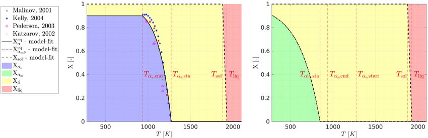
fraction Xαs over time (at constant temperature), the factors i) and ii) together result in the characteristic S-shape of
such diffusion-based processes as exemplary depicted in Figure 2 for four combinations of k and c. Depending on the
type of diffusion process, different values for the exponent cαs can be derived from the underlying physical mechanisms
resulting in more process-specific types of diffusion equations. In its most general form, which is applied in this work,
the exponent cαs of the modified logistic differential equation is kept as a free parameter, which allows an optimal
inverse identification based on experimental data even for complex diffusion processes [43].
When cooling down (Ṫ < 0) the material at temperatures below the Martensite start temperature (T < Tαm ,sta ) and the
equilibrium composition of the stable αs -phase has not been reached yet (Xαs < Xeq α ), an instantaneous Martensite
formation out of the (excessive) β-phase is assumed following the Martensite pseudo equilibrium composition Xeq αm
according to (5). Mathematically, this modeling assumption can be expressed by an inequality constraint based on the
following Karush-Kuhn-Tucker (KKT) conditions:
Xαm − Xeq
αm ≥ 0 ∧ Ẋβ→αm ≥ 0 ∧ (Xαm − Xeq
αm ) · Ẋβ→αm = 0. (11)
7A PREPRINT - JANUARY 15, 2021
1.0
0.8
0.6
X [−]
0.4
k = 0.1, c = 2.0
0.2
k = 0.3, c = 2.0
k = 0.1, c = 4.0
k = 0.3, c = 4.0
0.0
0 20 40 60 80 100
[]
t s
Figure 2: Four exemplary phase evolutions of a nucleation process modelled with Equation (10) with initial phase
fraction X0 = 0, equilibrium Xeq = 1 and combinations of k ∈ {0.1, 0.3} and c ∈ {2.0, 4.0}.
The constraint Xαm −Xeq αm ≥ 0 (first inequality in (11)) states that Xαm cannot fall below the equilibrium composition
Xeq
αm since Martensite will be formed instantaneously out of the β-phase. Here, the formation rate Ẋβ→αm (second
inequality in (11)) plays the role of a Lagrange multiplier enforcing the constraint Xαm −Xeqαm = 0 as long as Martensite
is formed. According to the complementary condition (third equation in (11)), this formation rate vanishes in case
of excessive Xαm -phase (i.e. Ẋβ→αm = 0 if Xαm − Xeq αm > 0). This scenario can occur e.g. during heating of the
Martensite material (i.e. Ẋeq
αm < 0) since the diffusion-based Martensite-dissolution process (see below) cannot follow
the decreasing equilibrium composition Xeq αm in an instantaneous manner.
Since the αm -phase is energetically less favorable than the αs -phase, there is a driving force for the transformation
αm → αs . In contrast to the instantaneous formation of Martensite, the αm -dissolution to αs is modeled as (time-delayed)
diffusion process [6] according to
cαs −1 cαs +1
(
eq cα
Ẋαm →αs = k α s (T )·(X αs ) cα s
· X α m − X̄ α m
s for Xαm > X̄eq
αm , (12)
0 else,
where X̄eqαm = 0 represents the long-term equilibrium state (t → ∞) of the Martensite phase (see Equation (7)).
Equations (10) and (12) have the same structure and share the same exponent cαs as well as the same diffusion rate
kαs (T ) since both describe the diffusion-based formation of αs -phase, i.e., both result in the same daughter phase. The
underlying modeling assumption is that the transformation αm → αs can be split according to αm → β → αs , i.e., it is
assumed that Martensite first dissolves instantaneously into the intermediate phase β, which afterwards transforms to
the αs -phase in a diffusion-based β → αs process similar to (10). The model for the temperature-dependence of kαs (T )
as described below will result in diffusion rates that drop to (almost) zero at low temperatures such that Martensite is
retained as meta-stable phase at room temperature, which is in accordance to the corresponding experimental data.
Eventually, also the case of lacking β-phase (i.e., Xβ < Xeq β ) shall be considered: Due to the nature of the β-dissolution
processes Ẋβ→αs according to (10) and Ẋβ→αm according to (11), which only yield contributions as long as Xβ > Xeq β,
eq
this scenario can only arise from Ẋβ > 0, i.e., if Ṫ > 0 and T ∈ [Tαs ,end ; Tαs ,sta ].
Experimental data by Elmer et al. [34] strongly supports a diffusional behavior of β-phase build up, respectively
αs -dissolution during heating of Ti-6Al-4V. We thus chose a diffusional nucleation model in Equation (13) for the
8A PREPRINT - JANUARY 15, 2021
resulting αs → β transformation:
cβc −1
cβc +1
β
· Xα − Xeq , for Xα > Xeq
Ẋαs →β = kβ (T ) · X̃β α β
α (13)
0, else.
Here, X̃β = Xβ − 0.1 defines a corrected β-phase fraction. This ensures that the second factor in (13), which can be
interpreted as a measure for the increasing diffusion interface during the formation process, starts at a value of zero
when heating material with initial equilibrium composition Xβ = Xeq β above Tαs ,end . By this means, the temporal
evolution of X̃β (i.e., of the additional β-material beyond 10%) begins with a horizontal tangent when exceeding Tαs ,end
as also observable in corresponding experiments [34]. From a physical point of view this experimental observation - as
well as the corresponding diffusion model in (13) - rather correspond to a phase nucleation and subsequent growth
process of a new phase fraction X̃β (starting at X̃β = 0) than a continued growth process of a pre-existing phase
fraction Xβ (starting at Xβ = 0.1). While existing experimental data in terms of temporal phase fraction evolutions is
very limited, there is still significant experimental evidence that the αs → β dissolution should be considered as a
(time-delayed) diffusion-based process [4, 34] rather than an instantaneous transformation, which for simplicity has
been assumed in some existing modeling approaches, like e.g., [6].
Let us again consider the case of lacking β-phase (i.e. Xβ < Xeq β ), which can only occur in the temperature interval
T ∈ [Tαs ,end ; Tαs ,sta ] as discussed in the paragraph above. If in this scenario, a certain amount of remaining Martensite
material (i.e. Xαm > 0) exists, it is assumed that the αm -phase fraction is decreased in an instantaneous αm → β
transformation such that Xβ can follow the energetically favorable equilibrium composition Xeq β . Mathematically, this
modeling assumption can be expressed by an inequality constraint with the following KKT conditions:
If Xαm > 0 : Xβ − Xeq
β ≥0 ∧ Ẋαm →β ≥ 0 ∧ (Xβ − Xeq
β ) · Ẋαm →β = 0. (14)
The constraint Xβ −Xeq
β ≥0 (first inequality in (14)) states that Xβ cannot fall below the equilibrium composition Xeq β
as long as a remainder of Martensite, instantaneously transformable into Xβ , is present. Again, the formation rate
Ẋαm →β (second inequality in (14)) plays the role of a Lagrange multiplier enforcing the constraint Xβ −Xeq β = 0 as long
as the αm → β transformation takes place. According to the complementary condition (third equation in (14)), this
formation rate vanishes in case of excessive β-phase (i.e. Ẋαm →β = 0 if Xβ −Xeq β > 0). Since in the considered scenario,
the remaining contributions to Ẋβ vanish, i.e., Ẋαs →β = 0and Ẋβ→αs = 0 due to Xβ = Xeq β as well as Ẋβ→αm = 0 due
to T > Tαm ,sta , (8c) together with the differential form of the constraint Ẋβ = Ẋeqβ allows to explicitly determine the
eq
corresponding Lagrange multiplier to Ẋαm →β = Ẋβ . Once all Martensite is dissolved, i.e., Xαm = 0, the β-phase
fraction cannot follow the corresponding equilibrium composition Xeq β in an instantaneous manner anymore, but rather
in a time-delayed manner based on the diffusion process (13).
To close the system of model equations proposed in this section, a specific expression for the temperature-dependence
of the diffusion rates kαs (T ) and kβ (T ) required in (10), (12) and (13) has to be made. The mobility of the diffusing
species, which is represented by these diffusion rates, is typically assumed to increase with temperature. However, it is
assumed that the diffusion rates do not increase in a boundless manner but rather show a saturation at a high temperature
level. Moreover, for the considered class of thermally-activated processes, these diffusion rates are assumed to drop
to zero at room temperature. The following type of logistic functions represent a mathematical tool for the described
system behavior:
k1
kαs (T ) := (15)
1 + exp [−k3 · (T − k2 )]
The free parameters k1 , k2 , k3 and cαs governing the β → αs -diffusion processes (10) and (12) will be inversely
determined in Section 3 based on numerical simulations and experimental data for time-temperature-transformations
(TTT). The same temperature-dependent characteristic as in (15) is also assumed for the αs → β-diffusion process (13).
Since the dissolution of αs - into β-phase is reported to take place at higher rates [4, 34] as compared to the αs -formation
out of β-phase, we allow for an increased diffusion rate kβ (T ) of the form:
kβ (T ) := f · kαs (T ) with f > 0. (16)
Thus, only the two free parameters f and cβ are required for the αs → β-diffusion. These two parameters will be
inversely determined in Section 3 based on heating experiments taken from [34].
9A PREPRINT - JANUARY 15, 2021
Remark (Martensite cooling rate). In our model the critical cooling rate Ṫαm ,min = −410 K/s is not prescribed
as an explicit condition for Martensite formation as done in existing microstructure modeling approaches [6,
40]. Instead, the process of Martensite formation is a pure consequence of physically motivated energy balances
and driving forces for diffusion processes. In Section 3.3 it will be demonstrated that a value very close to
Ṫαm ,min = −410 K/s results from the present modeling approach in a very natural manner when identifying
the critical rate for pure Martensite formation from continuous-cooling-transformation (CCT) diagrams created
numerically by means of this model.
Remark (Johnson-Mehl-Avrami-Kolmogorov (JMAK) equations). In other publications [4, 6, 19, 23, 27, 34,
40, 44], Johnson-Mehl-Avrami-Kolmogorov (JMAK) equations are used to predict the temporal evolution of
the considered phase fractions. It has to be noted that JMAK equations are nothing else than analytic solutions
of differential equations (for diffusion processes) very similar to (10), which are, however, only valid in case
of constant parameters kαs , Xαs and Xeq β . Since these parameters (due to their temperature-dependence) are not
constant for the considered class of melting problems, only a direct solution of the differential equations via
numerical integration, as performed in this work, can be considered as mathematically consistent. We furthermore
want to note that the mathematical form of JMAK equations, which involve logarithmic and exponential expressions,
is prone to numerical instabilities in practical scenarios, especially for the extremely high temperature rates that
appear in SLM processes. In contrast, the proposed algorithm in the following Section 2.3.2 has a simple and robust
mathematical character.
2.3.2 Temporal discretization and numerical algorithm
For the numerical solution of the microstructural evolution laws from the previous section, we assume that a temporally
discretized temperature field (T n , Ṫ n ) based on a time step size ∆t is available at each discrete time step n (e.g.
provided by a thermal finite element model as presented in Section 4.1). In principle, any time integration scheme can
be employed for temporal discretization of the phase fraction evolution equations from the last section. Specifically, in
the subsequent numerical examples either an implicit Crank-Nicolson scheme or an explicit forward Euler scheme have
been applied. For simplicity, the general algorithmic realization of the time-discrete microstructure evolution model is
demonstrated on the basis of a forward Euler scheme.
For the following time integration procedure of (8) it has to be noted that only the rates Ẋαm →αs , Ẋβ→αs , Ẋαs →β
corresponding to diffusion processes will be integrated in time. Instead of integrating the rates Ẋβ→αm and Ẋαm →β cor-
responding to instantaneous Martensite formation and dissolution processes, the associated constraints in (11) and (14)
will be considered directly by means of algebraic constraint equations. In a first step, assume that the temperature data
T n+1 , Ṫ n+1 of the current time step n + 1 as well as the microstructure data Xnαs , Xnαm , Ẋnαm →αs , Ẋnβ→αs , Ẋnαs →β of the
last time step n is known. With this data, the microstructure update is performed:
Xn+1 n n n n
αs = Xαs + ∆t(Ẋβ→αs + Ẋαm →αs − Ẋαs →β ) and Xn+1 n n
αm = Xαm − ∆tẊαm →αs . (17)
The time integration error in (17) might lead to a violation of the scope Xn+1 n+1
αs , Xαm ∈ [0; 0.9] of the phase fraction
variables. In this case the relevant phase fraction variable is simply limited to its corresponding minimal or maximal
value, respectively. Similarly, if Xn+1
α = Xn+1 n+1
αs + Xαm exceeds the maximum value of 0.9 the individual contributions
Xαs and Xαm are reduced such that the maximum value Xn+1
n+1 n+1
α = 0.9 is met and the ratio Xn+1 n+1
αs /Xαm is preserved.
n+1 n+1
Subsequently, the β-phase fraction is calculated from the continuity equation Xβ = 1 − Xα . Afterwards, the
updated equilibrium phase fractions Xeq,n+1
αs and Xeq,n+1
αm are calculated according to (3)-(5) with Xn+1
αs and T n+1
eq,n+1 eq,n+1
before the corresponding equilibrium composition Xβ = 1 − Xα s of the β-phase is updated. Next, a potential
instantaneous Martensite formation out of the β-phase according to (11) is considered as follows:
eq ,n+1 eq ,n+1
If Xn+1
αm < Xαm , Update: Xn+1
β ← Xn+1
β + Xn+1
αm − Xαm , (18a)
,n+1
Set: Xn+1
αm = Xeq
αm . (18b)
Similarly, a potential instantaneous Martensite dissolution into β-phase according to (14) is considered as follows:
,n+1 ,n+1
If Xn+1
β < Xeq
β ∧ Xn+1
αm > 0, Update: Xn+1 n+1 eq
αm ← Xαm + Xβ − Xn+1
β , (19a)
,n+1
Set: Xn+1
β = Xeq
β . (19b)
Again, if necessary the increment in (19a) is limited such that the updated phase fraction Xn+1 αm does not become
n+1 n+1 n+1
negative. As a last step, the diffusion-based transformation rates Ẋβ→αs , Ẋαm →αs and Ẋαs →β according to (10), (12)
10A PREPRINT - JANUARY 15, 2021
and (13), all evaluated at time step n + 1, are calculated. With these results, the next time step n + 2 can be calculated
starting again with (17).
Remark (Initial conditions for explicit time integration). While the diffusion process according to Equation (12)
will start at a configuration with Xαm 6= 0 and Xαs 6= 0, Equation (10) needs to be evaluated for Xαs = 0 to initiate
the diffusion process. However, the evolution of Equation (10) based on an explicit time integration scheme will
remain identical to zero for all times for a starting value of Xαs = 0. Therefore, during the first cooling period
the phase fraction has to be initialized at the first time step tn where Xeq
α > 0. In the following, the initialization
procedure considered in this work is briefly presented. In a first step, (10) is reformulated using the relations
Xβ = 1 − Xα and Xeq eq eq
β = 1 − Xα as well as the approximate assumptions kαs (T ) = const., Xα = const. and
Xαm = 0 (i.e., Xα = Xαs ) for the initial state [43]:
cαs −1 cαs +1
Xα
ġ = k̃ · g cαs
· (1 − g)cα s
with g = , k̃ = kαs · Xeq
α. (20)
Xeq
α
Based on the analytic solution in [43], evaluated after one time step ∆t, the initialization for Xnαs at tn reads:
cαs −1
n eq cαs
Xαs = Xα · 1 + . (21)
k̃∆t
We compared this approach with an implicit Crank-Nicolson time integration (either used for the entire simulation
or only for initialization of the first time step), where the initial αs -phase fraction Xαs does not need to be set
explicitly and found no differences in the resulting diffusion dynamics according to (10).
3 Inverse parameter identification and validation of microstructure model
The four parameters θ diff,αs = [cαs , k1 , k2 , k3 ]T according to Equations (10), (12) and (15) as well as the two parameters
θ diff,β = [cβ , f ]T according to Equations (13) and (16), are so far still unknown and need to be inversely identified
via experimental data sets. For the inverse identification of θ diff,αs , we use so-called time-temperature-transformation
(TTT) experiments, a well-known experimental characterization procedure for microstructural evolutions [4, 6, 44, 45].
As TTT-experiments only capture the dynamics of cooling processes, we will identify the parameters θ diff,β governing
the heating dynamics of the microstructure via data from heating experiments taken from [34].
3.1 Inverse identification of αs -formation dynamics via TTT-data
Time-temperature transformation (TTT) experiments [46] are one of the most important and established procedures
for (crystallographic) material characterization. The goal of the TTT investigations is to understand the isothermal
transformation dynamics of an alloy by plotting the percentage volume transformation of its crystal phases over time.
Thereto, the material is first equilibriated at high temperatures such that only the high-temperature phase is present.
Afterwards, the material is rapidly cooled down to a target temperature at which it is then held constant over time so that
the isothermal phase transformation at this temperature can be recorded. Rapid cooling refers here to a cooling rate that
is fast enough so that diffusion-based transformations during the cooling itself can be neglected and can subsequently
be studied under isothermal conditions at the chosen target temperature. The procedure is repeated for successively
reduced target temperatures. The emerging diagram of phase contour-lines over the T × log(t) space is commonly
referred to as TTT-diagram.
In the present work, the simulation of TTT-curves for Ti-6Al-4V was conducted as follows: We initialized the
microstructure state at T = 1400 K > Tαs ,end with pure β-phase, such that Xβ = 1.0. Afterwards, the microstructure
was quickly cooled down with Ṫ = −500 K/s1 to a target temperature Ttarget ∈ [350, 1300] and the evolution of the
microstructure at this target temperature was recorded over time. The range of target temperatures was discretized in
steps of 10 K such that 95 individual target temperatures and hence microstructure simulations were considered. Figure
3 depicts the isolines of simulated Xαs - (left) and Xαm -phase fractions (right), after identifying the model parameters
via the experimental data [4, 6, 44, 47] shown in the left figure. Please note that the phase-fractions in Figure 3 were
normalized with Xeq α (T ), which takes on a value of 0.9 for temperatures below Tαs ,end , as this was also the case in the
underlying experimental investigations. We highlighted three temperatures T = {400, 800, 1000} K to discuss the
microstucture evolution at these points.
1
We chose a constant cooling rate here as the detailed cooling dynamics are not important for TTT diagrams as long as cooling
takes place "fast enough". In the latter respect, we also investigated several higher cooling rates without observing differences in the
resulting TTT-diagrams.
11A PREPRINT - JANUARY 15, 2021
TTT-diagram for X s
TTT-diagram for X m
T s, st a = 1273 K T s, st a = 1273 K
1200
0.010
0.050 0.450
0.990
0.950
0.550
T = 1000 K T = 1000 K
1000
T s, end = 935 K T s, end = 935 K
T m , st a = 848 K T m , st a = 848 K 0.010
T [K ]
T = 800 K 0.050 T = 800 K
800
0.450
0.550
600 Malinov (resist ivit y, 2001): X s = 0.05
Malinov (resist ivit y, 2001): X s = 0.01
Kelly: X s = 0.01
Malinov (resist ivit y, 2001): X s = 0.5
Malinov (resist ivit y, 2001): X s = 0.95
T = 400 K T = 400 K
400 Malinov (resist ivit y, 2001): X s = 0.95
0.950
10 -3 10 -2 10 -1 10 0 10 1 10 2 10 3 10 4 10 5 10 -3 10 -2 10 -1 10 0 10 1 10 2 10 3 10 4 10 5
t [s] t [s]
Figure 3: Simulation of the TTT-diagram for the αs - and αm -phases using the maximum likelihood point estimate
for the uncertain kinetic parameters θ ∗diff,αs of the microstructure evolution, along with experimental data by Malinov
[47] and Kelly [37]. Left: Contour-lines for Xαs ; Right: Contour-lines for Xαm . Contour lines are shown for the 1%,
5%, 45%, 55%, 95% and 99% normalized phase fractions. Three temperatures are marked in red and discussed in the
analysis.
At T = 1000 K (between Tαs ,sta and Tαs ,end , i.e. above Tαm ,sta ) we get a pure β → αs transformation. When looking
at higher target temperatures T > 1000 K it can be observed that the isoline with 1% phase fraction for Xαs is shifted
to longer times, which results from a decreasing value of Xeq α (i.e. a decreasing driving force) that slows down the
initial dynamics of Xαs -formation at elevated temperatures, even-though kαs is already saturated at its maximal value in
this temperature range (see Figure 4). At T = 800 K we are now below Tαm ,sta , so that the initial cool-down results
(instantaneously) in a Martensite phase fraction according to Xeq αm . With ongoing waiting time, the remaining β-phase
transforms in a diffusion-driven manner into stable αs -phase. In the TTT-diagram, we can already notice that the isoline
with 1% phase fraction for Xαs is shifted to longer times as compared to the higher temperature level T = 1000 K,
which, this time, is caused by the decreasing value of kαs for lower temperatures, as depicted in Figure 4 and modeled
in Equation (15). Moreover, the right-hand side of Figure 3 shows that the Martensite phase fraction decreases again for
waiting times t > 100s, which represents the diffusion-based dissolution of Martensite into αs -phase according to (12).
Finally, the transformation at T = 400 K initially results in almost the maximal possible amount of Martensite
(Remember: The 100%-isoline in Figure 3 corresponds to a phase fraction of 0.9 for T < Tαs ,end ). As the diffusion
rate kαs is almost zero for such low temperatures, the Martensite phase cannot be dissolved to stable αs in finite times
and the Martensite phase remains present as metastable phase at low temperatures, which agrees well with experimental
observations. In the TTT-diagram this effect shifts the isolines asymptotically to t → ∞ when approaching the room
temperature. All in all, the shift to longer times due to a low value of kαs for low temperatures and the delay effect due
to a decreasing (driving force) value of Xeq α at high temperatures leads to the typical C-shape of TTT-phase-isolines.
Inverse parameter identification was conducted for the diffusion parameters θ diff,αs by maximizing the data’s likelihood
for θ diff,αs . We assumed a (conditionally independent) static Gaussian noise for the measurements on the log(t)-scale.
This assumption is equivalent to a log-normal distributed noise in the data along the time-scale. The maximum-
likelihood point estimate can then be determined by solving the following least-square optimization problem (see
Remark below for more details):
X 2
∗
θ diff,αs = argmin Xαs ,TTT (log(ti ), Ti , θ diff,αs ) − Xαs ,TTT,exp.,i (22)
θ diff,αs i
In Equation (22) the term Xαs ,TTT (log(ti ), Ti , θ diff,αs ) describes the simulated TTT-phase fractions (normalized
by Xeq
α (T )) at time ti , Temperature Ti and for diffusional parameters θ diff,αs . The index i marks here the specific
temperatures and times for which the corresponding observed experimental data Xαs ,TTT,exp.,i was recorded.
12You can also read