Master Thesis Czech Technical University in Prague Faculty of Mechanical Engineering Department of Instrumentation and Control Engineering

Czech Technical University in Prague
 Faculty of Mechanical Engineering
Department of Instrumentation and Control Engineering

 Master Thesis

 Student
 Bc. Nikita Zhdankin

 Supervisor
 Ing. Matouš Cejnek, Ph.D.
 2020/2021

ii

Statement

I declare that I have worked out this thesis independently assuming
that the results of the thesis can also be used at the discretion of the
supervisor of the thesis as its co-author. I also agree with the
potential publication of the results of the thesis or of its substantial
part, provided I will be listed as the co-author.

Prague ……………………………

Signature ……………………………………………

 iii

Abstract
The goal of the thesis was to evaluate factors affecting football match results, create a
rating which would rank the football teams in an objective way and try to predict football
match results better than existing methods.

Firstly, several factors were evaluated in a way to what extent each factor affects a football
match result. Such factors as home advantage, age, form, motivation, average ball
possession and transfer values were evaluated. The results showed that the home
advantage is the most important factor in a football match as the team’s chances to win
almost double if it plays at a home ground.

Then, several predicting models were evaluated. I started with the Elo ranking system,
which was improved by implementing the factors which were described previously. This
system showed better predictability compared to the Poisson distribution model and
betting odds.

Finally, machine learning models were tested using historical data and the Elo ranking
system together with several of the factors. The results showed accuracy of 0.535, which
means that it would predict 53.5% of the games correctly.

 iv

Acknowledgements
Firstly, I would like to thank Ing. Matouš Cejnek, for being my supervisor during my work on
this master thesis and helping me throughout the whole year. Also, for the classes of
Python, which gave me knowledge during the course.
I want to thank my parents and my sister who were supporting me during the whole period
of my studies and especially last year which was stressful due to the pandemic.
I also want to thank all my friends and my girlfriend who were motivating, encouraging, and
supporting me.

 v

Contents

Introduction ............................................................................................................................................ 1
 Football ............................................................................................................................................... 1
 Odds .................................................................................................................................................... 3
ELO .......................................................................................................................................................... 5
 History ................................................................................................................................................. 5
 Mathematics ....................................................................................................................................... 5
 Elo model in football ........................................................................................................................... 8
 3 points for a win .............................................................................................................................. 10
Statistics ................................................................................................................................................ 12
XG .......................................................................................................................................................... 13
Factors affecting a result of football match .......................................................................................... 16
 Home advantage ............................................................................................................................... 16
 Age .................................................................................................................................................... 24
 Form .................................................................................................................................................. 27
 Motivation......................................................................................................................................... 29
 Ball possession .................................................................................................................................. 31
 Red cards........................................................................................................................................... 34
 Transfer values .................................................................................................................................. 36
Improved Elo model .............................................................................................................................. 39
 Formulae ........................................................................................................................................... 39
 Model ................................................................................................................................................ 40
Machine learning .................................................................................................................................. 42
 Definition .......................................................................................................................................... 42
 Experiment ........................................................................................................................................ 44
 Results ............................................................................................................................................... 46
Poisson .................................................................................................................................................. 48
 Definition .......................................................................................................................................... 48
 Experiment ........................................................................................................................................ 49
 Results ............................................................................................................................................... 49
Conclusion ............................................................................................................................................. 50
Future work........................................................................................................................................... 51
Probable uses ........................................................................................................................................ 51

 vi

List of tables
Table 1 – Meaning of odds

Table 2 – K-factor for FIFA World Rankings

Table 3 – Bundesliga, 2014, final number of points predictions

Table 4 - average final number of points predictions

Table 5 – average xG per shot

Table 6 – home performance of the most supported clubs

Table 7 – streak selection bias

Table 8 – results of the experiment on form affecting team’s performance

Table 9 – data used for the experiment

Table 10 – ball possession experiment results

Table 11 - ball possession experiment results

Table 12 – red card experiment results

Table 13 – percentage of domestic players in top football clubs

Table 14 – improved Elo model performance in English league

Table 15 – improved Elo model performance combined

Table 16 – Baseline models regression results

Table 17 – Baseline models classification results

Table 18 – Tuned models regression results

Table 19 – Tuned models classification results

Table 20 – Attendance at league matches and early cup matches

 vii

List of figures
Figure 1 - Luck-skill continuum

Figure 2 – Elo rating distribution

Figure 3 – Elo Logistic curve

Figure 4 – correlation between Elo difference and win probability

Figure 5 – testosterone levels of football players

Figure 6 – travel distance affecting home performance

Figure 7 – UD Las Palmas home performance and location on the map

Figure 8 – CS Maritimo and CD Nacional home performance and location on map

Figure 9 – Average attendance affecting home performance

Figure 10 – average age affecting average performance

Figure 11 – average age affecting performance of teams in different championships

Figure 12 - how motivation affects performance

Figure 13 – ball possession causing correlation with the number of goals scored

Figure 14 – how players wages affect team’s performance

 viii

1. Introduction
1.1. Football
Football is a game played with two opposing teams of 11 players and a ball for 90 minutes
[1]. The aim of each team is to score the ball into the opponent’s goals more times than the
opposing team does. If both teams have scored the same number of goals, the game ends in
a draw. Any country usually has a domestic league where a fixed number of clubs play
against each other. The team with the highest number of points at the end of the season
wins the league and 1 or more teams with the lowest number of points are relegated to the
lower division and replaced with the best teams of the lower division.

With big money coming into the sport, detailed statistics became crucial in reaching better
results. In recent years, new types of data have been collected for many games in various
countries, including information on each shot or run made in a match. The collection of this
data has made data science one of the most important fields of the football industry with
many possible applications: scouting players, improving match tactics, improvements in the
training process, injury prevention, betting and many more.

The first part of the thesis is determining which factors and to what extent affect the
football game results. The list of the factors would contain several uncontrollable or/and
unmeasurable ones, such as luck, mood of the players etc. Michael J. Mauboussin explains
the factor of luck in his book “The Success Equation” [2]. He put several kinds of sports on
so-called luck-skill continuum where on the left edge it has sports that depend only on luck,
such as roulette, and on the right edge there are sports that depend only on skill, such as
chess. The graph is presented below:

 Figure 1 - Luck-skill continuum [2]

 1

As the average number of goals scored in football is between 2.5 and 3, which is relatively
small, the sport is strongly affected by the factor of luck. Michael J. Mauboussin explains
that the higher the ratio of luck to skill in the sports the larger the sample needed to make
reasonable conclusions. For example, an Olympics champion in sprinting would beat an
amateur runner literally every time in normal conditions, but when moving left on the scale
above, it would require larger and larger sample to understand the contribution of skill.
Football is in the middle of the scale.

I will focus on controllable and measurable factors in this thesis. The list of the factors which
are going to be evaluated as follows:

 • Teams’ strength
 • Home advantage
 • Average ball possession
 • Recent form
 • Motivation
 • Age

The second part of this work is creating a model. It is going to be based on the ELO rating
model, but with several adjustments according to the results of the experiments on factors
listed above. The Elo rating model will be explained in the chapter ‘Elo’.

The third part will be about the Poisson distribution and how well it can predict the football
match results. After that, the machine learning models are going to be evaluated in
prediction of football matches. Several algorithms are going to be used and my updated Elo
ratings are also going to be used.

In the end, I will compare all the created models in order to find the best one. The overall
goal of the work is to objectively evaluate football teams as precisely as possible and try to
find a model which has the best chances of predicting a football match result correctly.

In my experiments I am going to use databases provided by sources like football-data.co.uk,
footystats.com and https://github.com/jalapic/engsoccerdata. The software used to
perform the experiments is Python 3.9 and the IDE used is PyCharm by JetBrains with a
student license provided by CTU in Prague.

 2

1.2. Odds
Betting is one of the biggest markets in the football industry. Odds represent the probability
of an event occurring [3]. For any given event, there are a certain number of outcomes. Take
rolling a dice for instance. If someone rolls a dice, there are six possible outcomes.
Therefore, if you bet that the person rolls a ‘one’, there is a 16.67% chance that will happen.
The price shown translates into a percentage chance of something happening or not.

The formula for transforming odds to probability is:

 1
 = ∗ 100% (1)
 
Where P is probability and O is odds. The example of calculation is in the table below:

 Table 1 – Meaning of odds

Data analysis is the first and most crucial step in the process of calculating the odds.
Bookmakers hire specialists to compile all the data possible and make models to improve
predictability of events. They try to get the best tools possible and work with the best
software to ensure that they get objective statistical evaluation of each game and the
possibilities. These days there is too much information for human beings to follow, that is
why bookmakers create mathematical models to set and change odds automatically.

Even though the bookmakers have probably the strongest models for predicting football
results, it is not their objective to be correct in the predictions. Their goal is to make as high
a profit as possible, therefore, they set the odds in the way they would beat an average
better. Bookmakers use advanced algorithms to calculate how much cash flow would be
placed on a specific market.

 3

After bookmakers have calculated the odds and the predicted cash flow, they need to post
the odds. They adjust the odds with something that is called ‘margin’. This factor allows
bookmakers to make money. The bookmakers use the margin and provide overall odds that
are slightly lower than what they should be. If both outcomes have the same percent
probability, then the odds should be even - 2.0. But the actual odds are lower than the
conventional ones, which means that they might offer something slightly lower than 2.0
depending on their financial politics instead of even odds. The difference between the odds
is the margin itself. The margin varies between different bookmakers – usually from 3 to 10
percent.

In case of an event that could end with 3 different outcomes the margin can be calculated
using the following formula:

 1 1 1
 = ∗ 100 + ∗ 100 ∗ 100 − 100 (2)
 1 2 3

For example, for the World Cup 2018 Final, the odds were: 2.15 for France’ win, 4.23 for
Croatia win and 3.08 for the draw, so the margin could be calculated as follows:

 1 1 1
 = ∗ 100 + ∗ 100 ∗ 100 − 100 = 46.5 + 32.5 + 23.6 − 100 = 2.64 %
 2.15 3.08 4.23

The margin is much lower than usual because the World Cup Final is the biggest market.

The odds can change before the game due to injuries or some other issues within the teams.
The odds can also change during the match, because of events, like a red card, player
change, injury, penalty, goal, or other events that might change the match's outcome.
Another reason why the odds change is because of the cash projections that might affect
the bookmakers’ profit.

Even though the profit is the bookmakers’ goal, as was already mentioned, betting odds can
beat any existing mathematical model in predicting football results.

 4

2. ELO
2.1. History
The Elo rating was created by a Hungarian master-level chess player Arpad Elo, born in 1903
he won eight titles of Wisconsin State champion, but he is mostly known by the rating
system he created in 1960. Since the United States Chess Federation was founded in 1939
[4], it was willing to apply a rating system which would help members to track individual
progress. The Harkness system which was used from 1950 to 1960, used four digits and had
a top rating of about 2600, the reason for that was explained by its’ creator – Kenneth
Harkness – he felt that fewer digits would leave too many players with the same rating. The
Harkness system was considered inaccurate; therefore, it was replaced by the Elo rating,
and it is still in use by main chess federations including FIDE – World Chess Federation –
with minor adjustments. Initially Arpad wanted to decrease the rating of a “strong player”
from 2000 to 1000, but it appeared then that it would mean that some weaker player could
get a negative rating. That is why Elo has decided to roughly keep the scoring.

2.2. Mathematics
Elo rating’s central assumption is that the performance of the player (or team if we are
analysing football) is a normally distributed random variable [6], which means that 68% of
the values are within +/- one standard deviation of the mean, 95% are within +/- two
standard deviations, and 99.7% are within +/- three standard deviations. It is based on the
fact that the performance of a given player, or a team is not the same from game to game. It
can vary due to multiple uncontrollable factors, but the player’s true skill is the mean of his
performance random variable.

 5

Figure 2 – Elo rating distribution [5]

Graph above shows an example of player 1 (blue line), whose rating is 1300, competing
against player 2 (red line), whose rating is 1600. Judging by the graph, player 1 loses the
game in most of the cases, but if player 1 overperforms and player 2 underperforms, there
is a chance for player 1 to win a game.

 Figure 3 – Elo Logistic curve [5]

The graph above is called a Logistic curve. The Elo rating is designed so that if a player has a
rating that is 400 points more than an opponent player, he is 10 times more likely to win a
game. That is shown on the graph – the unshaded area under the curve is 10 times greater
than the shaded one. Therefore, if a player has a rating that is 800 points more than an
opponent, his likelihood to win a game is 100 greater. Putting that into the formula:

 6

 = 10( − )/400 ∗ (3)

Where PwinA and PwinB are the probability of winning of two players, RA and RB are their Elo
ratings accordingly. This formula can be rewritten as:

 = 10( − )/400 ∗ (1 − ) (4)

Modifying the formula above it is possible to get the first out of the two formulae that
original ELO rating is based on:

 1
 = − (5)
 1+10 400

Where OE is the expected outcome of the game, which is calculated using ELO rating of
teams A and B, and the higher the difference between these two numbers the higher the
probability of winning of the team with higher ELO rating. This dependence can be seen on
the graph below.

 Figure 4 – correlation between Elo difference and win probability

The second formula for original ELO rating is presented below:

 = + ( − ) (6)

Where Rnew is the ELO rating of a team after the match, Rprevious is the ELO rating of the team
before the match, K is weight index, O is the outcome of the match (1 if the team has won
the game, 0.5 if the game has drawn, 0 if the team has lost the game) and OE is the expected

 7

outcome which is calculated by the formula [3]. Using 1, 0.5 and 0 as values for the outcome
of the match assume that team A, for example, performed at a better level than team B in
the case of scoring more goals, which is not always the case. Therefore, the goal of my
model is to take into consideration the cases when a team dominated the game but did not
manage to transfer this domination into the goals due to bad luck, biased referee or some
other factors.

FIDE, The International Chess Federation, uses the following ranges for the K-factor:

K = 40, for a player new to the rating list until the completion of events with a total of 30
games and for all players until their 18th birthday, as long as their rating remains under
2300.

K = 20, for players with a rating always under 2400.

K = 10, for players with any published rating of at least 2400 and at least 30 games played in
previous events. Thereafter it remains permanently at 10.

2.3. Elo model in football
The goal of this work is to modify the formulae so that the updated Elo rating would give
much accurate rating of the football teams.

There are several existing Elo models that are applicable for football. http://clubelo.com is
the first example, two main formulae for their rating are the same as for the original Elo
rating with weight index K = 20. One modification by the website is weighting goal
difference. This is implemented via using the following formula:

 = 1 ∗ √ (7)

Where:

 _1 2
 _1 = (8)
 ∑(√ ∗ )
 1 2

Where ΔElo_1X2 is the number of points that teams exchange after the result of the game is
known, pmargin is the likelihood for a specific margin, p1X2 is the likelihood to win (or lose) by
any margin. The sum is over all margins for a win or all margins for a loss.

 8

Another modification for this rating is Home Field Advantage (HFA). ClubElo increases the
Elo difference for a match by a certain number of Elo points. Every day and for every
country separately, the system compares if home teams won more or less points than away
teams. If home teams won more, HFA is increased, if away teams won more points, HFA is
decreased according the following equation:

 += ∑ ∗ 0.075 (9)

Elo rating for football is also used by the website http://eloratings.net and FIFA World
Rankings [7]. Both do not take into account home advantage. FIFA World Rankings do not
even have goal margin in the formulae, but both ratings consider importance of the
tournament by changing K-factor:

 Table 2 – K-factor for FIFA World Rankings [7]

There are several problems with the Elo ratings. An increase or decrease in the average
rating over all players in the rating system is often called a rating inflation or rating deflation
accordingly. This phenomenon has been noticed in chess, where in July 2000 the average
rating of the top 100 players was 2644 and by July 2012 this number had increased to 2703.

The rating does not show the strength of the player or team but rather shows the ability
compared to other player or team of the championship they compete against each other.

Initially the Elo model has assumed that only a win or a loss is possible. Addition of a draw
as a third possible outcome complicates the problem. The simplest way to model a
probability of a draw was described in a 1967 article by P. Rao and L. Kupper [8]. The model
assumes that the draw happens when the players or teams perform at a similar level. It is
supposed that there exists a number D which is the largest difference in strengths displayed

 9

in an individual game that would result in a draw, such that a probability of winning of team
A is:

 10 ⁄400
 = (10)
 10 ⁄400 +10( + )⁄400

As the chance of winning for team B is calculated by the same formula, it is possible to
calculate the probability of the draw by subtracting these two resulting values from 1. It is
going to be necessary to calculate the average percentage of games finishing as a draw and
to check if there is any correlation between team strength and frequency of draws.

Elo is not the only one rating system created. One of the most famous rating systems is the
so-called Glicko system created by Mark Glickman [9], who modified Elo rating by
introducing the rating deviation variable RD. The goal was to avoid cases when some players
played less frequently than others, therefore decreasing precision of the prediction by the
model. As my model predicts football matches, all clubs play the same amount of games, so
introducing rating deviation would not make any difference. The Glicko system also applies
a rating volatility σ to each player which defines how player performance varies from his
original rating.

J.Lasek, Z. Szlavik and S. Bhulai in their paper “The predictive power of ranking systems in
association football” [10] compared current FIFA Rankings for national teams with several
types of Elo ratings, least squares rating etc. They found that any of the Elo ratings would
give more accurate results than the official FIFA Rankings. The authors also point out that it
should be noticed by FIFA as the rankings affect the football competitions, for example, the
draws for international tournaments take into consideration national teams’ rating.
Therefore, it might be manipulated, for example, playing friendly matches with high
probability of increasing one team’s rating.

2.4. 3 points for a win
As it has been mentioned in a previous chapter, the Elo model uses the following points
system: win is 1 point, draw is 0.5 points and loss is 0 points. But in reality, in professional
football 3 points are awarded for a win, 1 point is awarded for a draw and the same 0 points
for a loss.

 10

Originally, two points for win were introduced when the football leagues were starting, and
it seemed like a reasonable decision [11]. That went on for more than 90 years, but in the
1980s, football was facing serious problems with attendance. The main reason for that
seemed to be that the teams value the draw point too much and would not risk going for a
win, making football seem boring. Crowds had almost halved in the early 1950s, and it was
clear that something had to be done. In the year of 1981 one of the English broadcasters
proposed the reward for win to three points. He received some criticism, that it would make
a winning team, after scoring a goal, want to sit on their lead even more than previously,
but the system of 3 points for a win was introduced anyway.

Research showed that applying three points for a win to every season going back to the
second world war, and in each case the champions would remain the same. In the five
seasons before the switch, there were an average of 133.0 draws per season in what was
then the league; in the five seasons after, there was an average of 113.4. The change seems
also to have promoted more attacking play. In the five seasons leading up to it, home teams
averaged 1.60 goals per game and away teams 1.01; afterwards home teams averaged 1.64
and away teams 1.07. That is a small change, but optimists could even argue that away
teams had become proportionally more attacking – suggesting they were less prepared to
play for draws.

A 2005 study by the economists Luis Garicano and Ignacio Palacios-Huerta deeply analysed
the effects the points system change had on football [12]. In this study the researchers
explained that it is not only about a decrease in the number of draws. The number of
matches decided by a large number of goals declined. Measures of offensive effort such as
shot attempts on goal and corner kicks increased while indicators of sabotage activity such
as fouls and unsporting behaviour punished with yellow cards also increased. Attacking
effort increased approximately the same degree as the number of fouls increased resulting
in an unchanged amount of goals scored. One more reason for that is assumed to be that
the losing team is less willing to score, because the one point awarded for a draw is worth
less in a new system.

In conclusion, two points for a win is going to be used in my thesis in order to comply with
the Elo model, which assumes that a win is worth twice as much as a draw.

 11

3. Statistics
Two big statistics analysis measurements that are going to be used a lot in this work are
correlation and regression. In this part of my thesis I am going to explain them in detail.

Correlation is used for a quick and simple summary of the direction and strength of the
relationship between two or more numeric variables [13]. Regression is used for prediction,
optimizing, or explaining a number response between the variables, how one variable
influences another one.

Both measurements can quantify direction and strength of the relationship, but only
regression is able to show cause and effect, predict and optimize the relationship.

Correlation can be spotted when a change to one variable is then followed by a change in
another variable, whether it be direct or indirect. Variables are considered uncorrelated
when a change in one does not affect the other. If two variables are moving in opposite
directions, like when an increase in one variable results in a decrease in another, this is
known as a negative correlation. Knowing how two variables are correlated allows for
predicting trends in the future. The main purpose of correlation, from the point of view of
correlation analysis, is to find out the association or the absence of a relationship between
two variables. The degree of association is measured by a correlation coefficient, denoted
by r. It is sometimes called Pearson’s correlation coefficient after its originator and is a
measure of linear association. If a curved line is needed to express the relationship, other
and more complicated measures of the correlation must be used.

Unlike correlation which can be defined as the relationship between two variables,
regression shows how they affect each other [14]. Regression analysis helps to determine
the functional relationship between two variables so that it is possible to estimate the
unknown variable to make future projections on events and goals. Regression formula is
presented below:

 = + ∗ (11)

Where a refers to the y-intercept, the value of y when x = 0 and b refers to the slope. In case
of several variables affecting one, multiple regression analysis is used.

 12

The formula for multiple regression is:

 = + ∗ 1 + ∗ 2 + ⋯ + ∗ (12)

The main difference between two measurements is that regression defines how x causes y
to change, and the results are going to change if x and y are swapped. In case of correlation,
x and y are variables that can be interchanged, and results stay the same.

 4. XG
Expected goals (xG) is a predictive model used to assess every goal-scoring chance [15], and
the likelihood of scoring a goal. Each shot on goal made is evaluated between 0 and 1. It
means that if a shot is 0.43 xG, out of 100 attempts the average player would score
approximately 43 goals.

There is no commonly accepted way to calculate xG of the shot. But it is known that most of
the sports analytics laboratories use following factors to evaluate a goal-scoring chance:

 • Distance to the goal
 • Angle to the goal
 • Which part of the body was a shot made with
 • Type of the shot (open-play, free-kick, corner, or counterattack)
 • Number of defenders between an attacker and a goal
 • Assist type (long ball or through ball)

Analytics companies use big historical data in order to construct a model with high accuracy.

The main assumption in the model is that every player has approximately the same finishing
skill in theory. In practice there are some players that would constantly score more goals
than xG model predicts them to score. But even the best finishers would not score more
than 20% higher than their xG, therefore, it would not affect my model.

xG is a sufficient way to indicate whether results are based on sustainable factors like a
constant creation of good chances, or whether it is down to aspects such as luck or good

 13

goalkeeping. For example, if a team is scoring more than it is predicted by the xG model, it is
expected that this team’s results would get worse due to regression to the mean. Surely, the
difference between goals and xG might just tell about the style of the team, but the
difference would still decrease over time. This factor I have evaluated in the following
experiment.

The data for the last 6 years for top-6 championships (Italy, England, Spain, France,
Germany, Russia) was gathered from the understat.com – 36 seasons in total. The goal of
the experiment was to find out which parameter predicts the final position of the team
better after half of the season: goals, xG or combination of both.

In order to use xG in table prediction it is necessary to introduce another metric called
xPoints (XP). It is basically just the expected number of points teams are going to get with
the xG number they got in a game between each other. For example, team A plays against
team B and according to xG, the possible outcomes of the game are team A win is 50%,
draw is 30%, team B win is 20%. XP is calculated [16] in this case as follows:

XP = [3* x (Possible Outcome of a win)] + [1 x (Possible Outcome of a Draw)] (13)

XPA = (3* x 0.5) + (1 x 0.3) = 1.8 (14)

XPB = (3* x 0.2) + (1 x 0.3) = 0.9 (15)

* in my experiment I use 2 points for a win system

The win probabilities are calculated using a Monte-Carlo Simulation.

Monte-Carlo Method is a mathematical technique [17] used to estimate the possible
outcomes of an uncertain event. It was invented by John von Neumann and Stanislaw and
was named after a famous casino city due to the element of luck that is a core to the
modelling approach, similar to the game of roulette. Monte-Carlo Simulation works in the
way that it predicts a set of outcomes based on an estimated range of values versus a set of
fixed input values. It builds a model of possible results by using a probability distribution,
such as a uniform or normal distribution, for any variable that has inherent uncertainty. It
recalculates the results multiple times, each time using a different set of random numbers
between the minimum and maximum values. Usually this exercise can be repeated
thousands of times to produce a large number of likely outcomes.

 14

In order to find out whether or not the xG model can help predict the football game result
The procedure of the experiment consisted of getting data from the first half of each of 36
seasons analysed and predicting the final position of each club based on one of three
factors: points, xPoints and 1:1 combination of both. Once again, 2 points were awarded for
the win and 1 point was awarded for the draw. The process of the experiment has shown
below on the example of Bundesliga 2014 season:

 Table 3 – Bundesliga, 2014, final number of points predictions

After finding an average of the results of the experiments on all 36 seasons using the script
‘xpvspoints.py’ the following results were obtained:

 Table 4 - average final number of points predictions

As it was observed, xPoints showed the worst prediction of the future results while
combination of using both points and xPoints showed better prediction, but the prediction
based only on points is statistically insignificantly worse, even when different proportions in
the combinations are used. One more problem with xG is that the sample is relatively small,
therefore, it is decided not to use xG in the improved Elo model.

One more problem with the xG model is that open data usually provides just the final value
of xG for a single match, for example, team A finished the game with several shots worth 0.7

 15

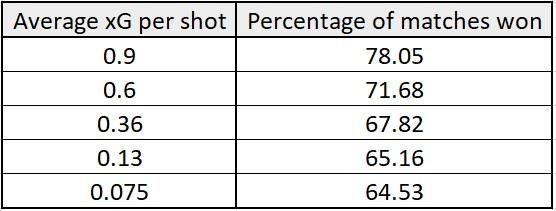
xG in total and team B with 1.8 xG. But there is a correlation between how dangerous each
of the shots were. In order to show this correlation, I have conducted an experiment based
on the Monte-Carlo Simulation.

In my experiment I have assumed that team A has done 4 shots: 0.3 xG, 0.2 xG, 0.1 xG and
xG. These numbers were fixed during the simulations. Team B shots were an independent
variable, the sum of the xG was the same – 1.8 xG, only the average xG per shot and number
of shots were changed. The number of simulations was 100000 for each experiment. The
results are presented below:

 Table 5 – average xG per shot

The results of the experiment prove that the sum of the xG for the match does not show the
full picture of the match and such stat as xG per shot would increase the accuracy of the
model.

 5. Factors affecting a result of football match
5.1. Home advantage
One of the most important affecting the football match and its result is so-called “home
advantage”. It means that if a team plays “at home”: in the city the club is based on, on the
stadium the team plays half of its game during the season. In this part of the thesis I am
going to discuss what exactly gives the home advantage and to what extent it affects the
result of the football match.

For the experiment data was used from 2014 to 2018 years. Data for 2019 and 2020 was
excluded as it was hugely affected by the crisis caused by coronavirus. As stadiums stopped

 16

allowing supporters to come to football matches, it has illuminated one of the main factors
causing home advantage – fans support.

It is necessary to find the percentage of games won by home teams. This was done by the
code named ‘home_win_percentage.py’. It calculated the combined win rate from all
championships involved in the experiment, excluding last two years data for the reasons
described above. The results for the home teams were as following:

Average win rate is 49.62 %

Average draw rare is 25.72 %

Average loss rate is 24.66 %

As seen above, it can be surely said that home advantage is something very significant in any
football match. Home teams are winning approximately twice more often than the away
teams. In football leagues and cups this effect is illuminated as usually in leagues when each
team must play with each team, they play 2 times: home and away.

In cups with a play-off system, the final is usually one match which is played on a ‘neutral’
pitch in order to avoid the case when one team has home advantage and another one
doesn’t.

It is also a known fact that 6 out of 18 FIFA World Cups were won by the hosting countries
[18]. It might be affected by the fact that earlier the World Cups were hosted by the most
powerful teams. But it is impossible to ignore such performances like Sweden (17th in the
1958 ELO Rating) getting to the final, Chile (23rd in the 1962 ELO Rating) getting to the semi-
final, Mexico (36th in the 1970 ELO Rating) getting to the quarter-final, USA (53rd in the 1994
ELO Rating) getting to the round of 16, South Korea (23rd in the 2002 ELO Rating) getting to
the semi-final, Russia (44th in the 2018 ELO Rating) getting to the quarter-final.

Reasons are considered to be different each time, for example, in South Korea in 2002
referees have made some questionable decisions leading Korea to the top-4 of the
tournament. [19] Mexico is several thousand meters above the water level, therefore lower
atmospheric pressure, which affects players performance. [20] The other case is the
overperforming of the Russian national team in 2018 which has probably been caused by
the motivation given from their fans’ support. [21]

 17

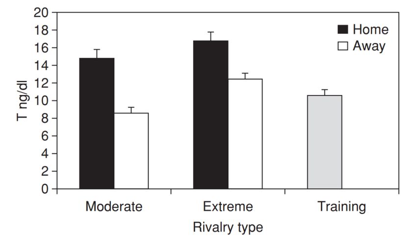
The studies on evolutionary psychology compare home advantage with ‘the protective
response to an invasion of one’s perceived territory’, it is proven by the testosterone levels:
for those who play at home it is significantly higher than The studies also show that the
home advantage is stronger at the time when a league has just been created and decreases
over time. [22] This fact may be ignored for this experiment as all considered leagues have
decades of history.

 Figure 5 – testosterone levels of football players [22]

Even though the home advantage is a combination of many factors, it is still possible to
evaluate some of them.

The experiment is divided to several parts to investigate which factor has more impact on
the home advantage, these factors are:

 • Distance which an away team has travelled to get to the football pitch
 • Match attendance
 • Geographical factors, such as area of the country and climate.

The data were taken from the most popular and most rich football nations, which are:
Argentina, Austria, Belgium, Brazil, China, Denmark, England, Finland, Germany, Greece,
Ireland, Italy, Japan, Mexico, Netherlands, Norway, Poland, Portugal, Romania, Russia,
Scotland, Spain, Sweden, Switzerland, Turkey, USA

Taking into consideration less popular championships might affect the results of the
experiment. For example, Nigerian Football League, season 2012/2013 [23]. The conditions

 18

are so unique, that top 16 teams in the table have not lost a single home game in the whole
season. The reasons for that are the following: referees are under threat if they make
decisions against the home team, even if those decisions are correct; violent home crowds;
dangerous and exhausting travel etc.

Data for the experiment was taken from the following websites: https://www.football-
data.co.uk/data.php and https://github.com/jalapic/engsoccerdata

The first main factor analysed is travel distance. It is assumed that the more time a visiting
travel spends on travelling the harder the game will be for them. When the travel distance is
high, it might also be the case of different climates or different time zones, which makes it
even more difficult to play for the away team.

The goal of the experiment was to find correlation between average travel distance for the
club throughout the season and the club’s average performance at home field.

The first step in the experiment was to get the data for chosen championships. The first part
of the data is the travel distance of each club. The procedure was as following:

 • Creating .csv documents with the list of the clubs that were playing at least one
 season in the championship during the time between 2014 and 2018. The code is in
 the file ‘clubs.py’
 • Creating .csv documents with the list of the clubs and the cities their home stadiums
 are in. The data were taken from https://en.wikipedia.org
 • Creating .csv documents with the list of the clubs, their home cities and longitude
 and latitude, the geographical data was received from https://latitudelongitude.org
 • Creating .csv documents with the list of clubs, their home cities, longitude and
 latitude, and the distance (in kilometres) the team travels throughout one season. It
 is calculated as the sum of distances between one and other cities in the file
 ‘calculating_km.py’
 • To compile average travel distance and average team performance at home file
 ‘calculate_win_percentage_club.py’ is used
 • To visualise the data for each championship the file ‘travel_vs_win_clubs.py’ is used.

 19

The findings of the experiment show that there is a correlation between how much the
team travels to play away or how much the opponent team travels to play this team and
how well the team performs at home during the season.

 Figure 6 – travel distance affecting home performance

The x-axis of the graph is average travel distance throughout the season, the y-axis is
average performance at home compared to average performance. The graph shows that
there is a correlation, which means that the more the team travels the better its’
performance at home rather than away.

Some more significant graphs are presented below.

 20

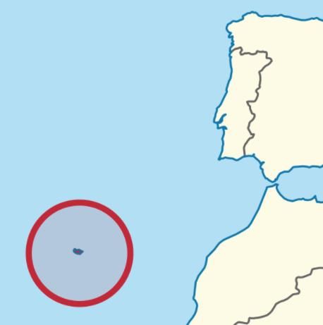
The first example is UD Las Palmas, a football club from Spain. It is based in the Canary
Islands on the Atlantic Ocean, significantly far from mainland Spain, therefore having
significantly higher at home performance comparing to other clubs in the league.

 Figure 7 – UD Las Palmas home performance and location on the map [24]

The first picture above shows where the UD Las Palmas is based on the map, the second
graph shows where this club is on the graph of average travel distance versus home
performance.

The second example are two clubs from Portugal: CS Maritimo and CD Nacional. Both clubs
are based on the island of Madeira located approximately 600 kilometres away from
mainland Portugal. Therefore, these two clubs have significantly higher home performance
due to long travel comparing to other clubs in the league.

 Figure 8 – CS Maritimo and CD Nacional home performance and location on map [25]

 21

The first graph above shows where CS Maritimo and CD Nacional are based on the map, the
second graph shows where these clubs are on the graph of average travel distance versus
home performance.

The next factor evaluated is the average attendance throughout the season.

The procedure of this experiment was as following:

 • Creating .csv documents with the list of the clubs that were playing at least one
 season in the championship during the time between 2014 and 2018. The code is in
 the file ‘clubs.py’
 • Creating .csv documents with the list of clubs with the average attendance of the
 home stadium. The data were taken from the website
 https://www.transfermarkt.co.uk
 • Creating .csv document with average attendance for each championship using
 ‘avg_attendance_for_each_championship.py’ file
 • The data is visualised then by using the file ‘attendance_vs_win_clubs.py’

 Figure 9 – Average attendance affecting home performance

Unfortunately, the results of the experiment did not show any correlation between average
attendance and performance at home field. It even showed slight negative correlation,
which is not what was expected before the start of the experiment. The explanation may be
that higher attendance means a more expensive stadium which in turn means a richer

 22

football club and therefore a stronger team. And stronger team would have a good away
performance as it would be easy for them to beat any opponent even at away field.

After experiment failure, it was decided to verify that at least teams with widely known
great support would show some correlation between attendance and home performance.
Several teams with ‘loudest’ [26] fans were listed, with average home performance and
average home performance for their championship.

 Table 6 – home performance of the most supported clubs

Surprisingly, even the football teams with the most active fan base usually perform worse at
home according to the graph above. Not even a single club could perform at home better
than on average. The sample is very small and objective to make a conclusion that an active
fan base affects negatively, but it is worth considering.

The correlation that could not confirm the initial assumption that higher attendance would
cause higher home advantage, could be explained in several ways.

In later years as the financial side of football has become more crucial and clubs have
started to gain as much income as possible, one of the solutions was to bring more people
to the stadiums. Therefore, stadiums became more family-oriented with new kinds of
entertainment during matchday, consultations with the community of supporters, flexible
pricing and creating family only areas in the stadium.

 23

For the biggest and most famous football clubs like Barcelona or Arsenal, a huge part of
people coming to matches are now tourists who came to visit Spain and the UK respectively,
for whom visiting the football match is like an attraction. The categories described above
would not make a difference for home or away teams, as it is considered that they would
not support any of the teams playing.

There were also some other parameters checked if they affect the home advantage. The
following parameters were picked:

 • Area of the country, which should correlate with the average distance travelled for
 the clubs.
 • Average attendance
 • Average temperature of the air throughout the year

The code for visualising the data is in the file ‘other_correlations.py’

The results did not show any significant dependency of the home advantage on any of the
factors above. There is a slight correlation for each of the factors. But it is hard to take it into
consideration due to the small size of the correlation. But it proves the point that the home
advantage is a huge combination of different factors which is also different for each country
and even for each game.

5.2. Age
Another factor that might affect the result of a football match is the age of the players. With
the modern technologies currently, it is possible for an athlete to give the best performance
for much longer time than previously, due to multiple researches in medicine, dietetics, and
others. In football this change is obvious, in the Champions League, main European football
tournament, an average age has increased from 24.9 to 26.5 years between 1992/1993 and
2017/2018 seasons.

Barça Innovation Hub in their article ‘The Influence of Age on Footballers’ Performance’
analyse several studies in order to understand more about how the players’ age affect one’s
performance level [27]. They concluded that there is a clear loss of physical performance for
players over 30 years old comparing to younger players. This was explained by the fact that

 24

older players’ total distance covered is 2% less on average than younger players. Much
higher difference was found for the number of sprints and fast races - decrease by 21% and
12% respectively.

However, the technical and tactical performance was found to be better in older players.
The percentage of successful passes is 3% to 5% higher in players over 30 compared to
younger players. It is possible that the decrease in physical performance of younger players
is compensated by an improvement in other skills such as decision making and game
intelligence.

The article concludes that the combination of youth and maturity in a squad of players may
be the best formula for success of a team. It would seem necessary to individualise as much
as possible the players’ preparation according to their age: they don’t all need the same
training to reach the best version of themselves. Besides, it is crucial to adapt players’
positions and roles in the game to bring up the best qualities from each player on the field.

In order to confirm the conclusions stated above, the following experiment was conducted.
The data of average age of a starting XI were taken from https://www.transfermarkt.co.uk,
and was plotted against the number of points the team gets. Average age of a team was
adjusted to an average age of the league and the number of points was calculated as an
average number of points per game throughout the season. The results of the experiment
showed no correlation between age and results of a team, correlation coefficient was
calculated as -0.00176. The script used was ‘ppgvsage.py’.

 25

Figure 10 – average age affecting average performance

It was also decided to divide the leagues into three categories according to the UEFA
Countries Coefficients. The experiment was then conducted for each of the three groups.
The results showed -0.0487 correlation coefficient for the first category (the best leagues), -
0.00505 for the second category and 0.0535 for the third category. The scripts are named
‘tierone.py’, ‘tiertwo.py’ and ‘tierthree.py’. It may be assumed that the worse the quality of
the league, the more success a team can get by having older and experienced players in the
squad. But the correlation is not sufficient to include the age into the final model.

 Figure 11 – average age affecting performance of teams in different championships

 26

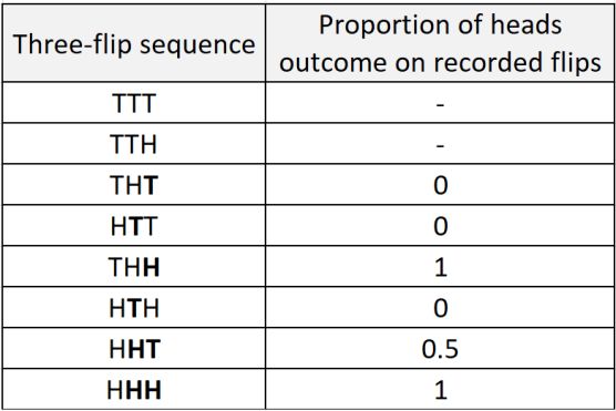
5.3. Form
One of the factors that might affect the result of a football match is the so-called “form” of
the teams. The concept is based on the idea that if a team is playing well or above
expectation, it is going to continue playing well due to increased self-confidence [28]. There
are not a lot of studies on that subject, but the book “Myths and Facts About Football”
suggests that this concept cannot be proved by numbers. In particular, the book study was
based on players, not teams, which is more important for creating a prediction model.
Therefore, the experiment on teams’ form is going to be conducted.

The study on players’ form might be questionable as it was discussed previously, football is
more affected by the factor of luck due to the low amount of shots on goal during the game.
Therefore, the study on basketball might be more significant, as the concept of form is
based on the factors that are also applicable for basketball. The number of attempts to
score a goal in basketball is high compared to other team sports, therefore, the data should
be more significant. For example, in the season 2018/2019 (the last season which was not
affected by COVID-19) the highest number of attempts for a player in English Premier
League was 137 by Mohamed Salah, and in the NBA the number was 1911 by James Harden.

The concept of form in basketball is called “Hot Hand” [29]. It was studied by Gilovich,
Vallone and Tversky in 1985. It was based on the assumption made by Kahneman and
Tversky in 1972 that people tend to overestimate representativeness of a small sample.
Scientists assumed that the Hot Hand is a misconception that would not be proved by the
numbers. After their assumption was not disproved by a research, they offered 26 people to
throw 100 balls in the net each from the positions with average success rate of
approximately 50% and then measured the number of successful and unsuccessful attempts
after a streak of successful shots. As the results showed that the number of shots scored
after successful streaks is about 50% the study concluded that Hot Hand was a myth.

After Big Data has entered basketball, the Hot Hand concept was revisited by Miller and
Sanjurjo in 2018 who wanted to verify if critics of 1985 study were right [30]. Besides several
obvious facts like small samples, poor experimental conditions, lack of defensive players etc,
scientists noticed that the mathematical approach itself was wrong. Gilovich, Vallone and

 27

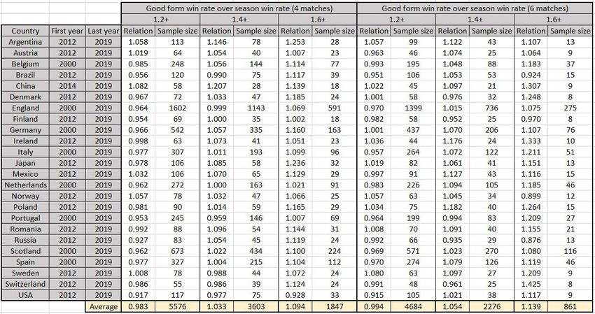
Tversky did not take into consideration a concept called streak selection bias which could be
explained by a coin flip. If a coin is flipped three times, there are eight different outcomes:

 Table 7 – streak selection bias [30]

According to the table above, the chance of getting head after head is 5/12, not ½ as it could
be expected. This bias could be prevented by larger samples. After Miller and Sanjurjo re-
evaluated the results of the 1985 experiment, they concluded that the hot hand is not a
myth. The explanation was as follows: Gilovich, Vallone and Tversky calculated the average
scoring of those 26 participants, which appeared to be 47%. Hot hand (scoring after 3
consecutive successful shots) had 49% probability and “Cold hand” (scoring after 3
consecutive unsuccessful shots) had 45% probability. But the error was to calculate the
average probabilities when participants had different numbers of streaks. For example, if
one player made 10 shots and scored 4 of them (40%) and another made 5 and scored 3
(60%), their average would be (7/15 = 45%), not ((40+60)/2=50%). The right method would
be to calculate an average of streaks, which would give the hot hand advantage up to 20%.

The conclusion above should be now proved experimentally for football. The experiment’s
procedure was as follows:

Data for several championships for multiple seasons was structured in a way that for each
football match there are several parameters for both teams: average points scored per
game before the current match, average points scored per game for the last 4/6 matches.
These numbers are chosen for the following reasons: the number should be even to avoid
home advantage, 2 matches sample is too small, 8 matches sample is too big and might be
affected by games played over a month ago. The number in the table represents the
relation between average points scored if a team is in good form and average points scored

 28

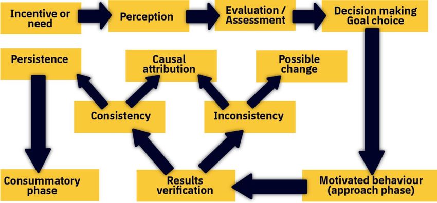
throughout the season. It is also necessary to notice that the points were calculated as 2
points per win for the reasons explained in the 2 points per win part of the thesis.

 Table 8 – results of the experiment on form affecting team’s performance

The results of the experiment show that if a team’s recent points per game are 1.4 times
higher than one throughout the season, it is 3-5% more likely to win a football match.
Accordingly, if a team’s recent points per game are 1.6 times higher than one throughout
the season, it is 9-14% more likely to win. In conclusion, form appears to be a significant
factor in a football match, therefore, it will be implemented in my prediction model.

5.4. Motivation
Motivation is another factor that affects the result of a football match. It refers to a
psychological feature that encourages a person to stay active and interested in a specific
goal, which in the case of a football game is to defeat the opposing team by delivering the
best performance possible [31]. The process that leads to this state of mind is complex and
briefly shown on the picture below:

 29