Modelling of Water Resources in the Brahmaputra River Basin - J. A. Bok April 2016

Modelling of Water Resources
in the Brahmaputra River Basin

 J. A. Bok

 April 2016

Modelling of Water Resources in
 the Brahmaputra River Basin

 MSc Thesis

 April 2016

 Author: Koos Bok

 Student number: 3537218

 E-mail: j.a.bok@students.uu.nl

 First supervisor: dr. ir. Geert Sterk (UU)

 Second supervisor: ir. Patricia Lopez Lopez (UU, Deltares)

 MSc programme: Master Earth Surface and Water

 Faculty of Geosciences

 Department of Physical Geography

 Utrecht University

Abstract In some parts of the world, network density of local hydro-meteorological station
data is lacking. A solution to this is to use satellite or reanalysis data. In the present study, different
interpolation techniques are applied to estimate precipitation and temperature using local observed
data and compared with global reanalysis WFDEI forcing data in the Brahmaputra River Basin. The
different forcing datasets were used to drive the global-scale hydrological PCR-GLOBWB model
to estimate discharge on a roughly 10×10 km spatial and daily temporal resolution. Discharge model
results were compared with observed records from the Bahadurabad gauging station. Results show
that the interpolated in-situ temperature forcing data is generally warmer than the WFDEI forcing
dataset. The interpolated in-situ precipitation forcing data consists of generally higher quantities
than the WFDEI forcing dataset, especially during the monsoon period. Discharge is underestimated
considerably using the WFDEI forcing dataset. Using the interpolated in-situ forcing data, the model
overestimates the discharge slightly. Several dataset combinations and data modifications were ap-
plied. The run with interpolated in-situ precipitation forcing data in the upper part of the basin and
WFDEI precipitation forcing data applied in the lower part of the basin, while using the interpolated
local temperature forcing data, produced the best result. This study concludes that the WFDEI forc-
ing dataset is useful and can provide reasonable estimates in combination with local hydro-
meteorological information.

 Keywords PCR-GLOBWB – WFDEI – Brahmaputra River Basin – Discharge – Monsoon

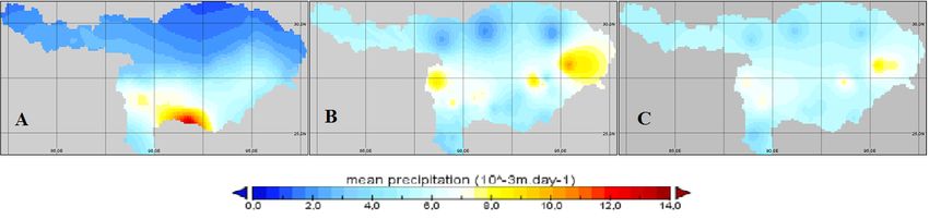
Table of Contents

1. INTRODUCTION ....................................................................................................................................... 1

 1.1. RESEARCH CHALLENGE ................................................................................................................................ 1
 1.2. RESEARCH OBJECTIVE .................................................................................................................................. 2

2. THE BRAHMAPUTRA RIVER BASIN ........................................................................................................... 3

 2.1. BASIN CHARACTERISTICS .............................................................................................................................. 3
 2.2. METEOROLOGICAL CHARACTERISTICS ............................................................................................................. 4
 2.3. HYDROLOGICAL CHARACTERISTICS.................................................................................................................. 6

3. RESEARCH METHODOLOGY ...................................................................................................................... 7

 3.1. HYDROLOGICAL MODEL: PCR-GLOBWB ....................................................................................................... 7
 3.1.1. Surface Runoff .............................................................................................................................. 8
 3.1.2. Vertical Water Exchange ............................................................................................................... 9
 3.1.3. Interflow ..................................................................................................................................... 10
 3.1.4. Baseflow...................................................................................................................................... 10
 3.1.5. Surface Water Accumulation and Routing.................................................................................. 10
 3.2. DATA DESCRIPTION ................................................................................................................................... 11
 3.2.1. Meteorological Forcing Data ...................................................................................................... 11
 3.2.1.1. WFDEI Dataset ........................................................................................................................................ 11
 3.2.1.2. In-situ Datasets ....................................................................................................................................... 12
 3.2.2. Observed Discharge Data............................................................................................................ 13
 3.3. COMBINED AND MODIFIED FORCING DATASETS ............................................................................................. 14
 3.3.1. Bias-Correction Method.............................................................................................................. 14
 3.3.2. Forcing Data Combinations ......................................................................................................... 15
 3.4. VERIFICATION STRATEGY ............................................................................................................................ 15

4. RESULTS ................................................................................................................................................. 17

 4.1. MODEL INPUT ANALYSIS ............................................................................................................................ 17
 4.1.1. Temperature ............................................................................................................................... 17
 4.1.2. Precipitation................................................................................................................................ 19
 4.2. EVAPOTRANSPIRATION .............................................................................................................................. 21
 4.3. SIMULATED DISCHARGE ............................................................................................................................. 23
 4.3.1. Initial Model Run Discharge Results ........................................................................................... 23
 4.3.2. Combined Dataset Model Runs .................................................................................................. 25

5. DISCUSSION AND CONCLUSIONS ........................................................................................................... 31

ACKNOWLEDGEMENTS .................................................................................................................................. 33

REFERENCES ................................................................................................................................................... 35

APPENDICES ................................................................................................................................................... 35

0

1. Introduction
Bangladesh, located in the Ganges-Brahmaputra-Meghna delta, acts as the drainage outlet for the whole
region. Annually, floods inundate large parts of the country imposing problems on water-related issues.
The location and the orography of the region makes the Brahmaputra River Basin especially vulnerable
to extreme events. Annual floods inundate approximately 20% of the country for a short time during the
monsoon season. During extreme floods, for example in 1998, more than 60% of the country was inun-
dated for nearly 3 months (Chowdhury, 2003; Mirza et al., 2003). In 1987 and 1988, similar events
occurred however with a smaller coverage and smaller duration. More recently, the years 2004, 2007,
and 2012 experienced extreme flooding. These events are primarily caused by intense monsoon precip-
itation (Mirza, 2003).
 The average discharge of the Brahmaputra is measured to be approximately 20,000 m3/s (Datta &
Singh, 2004; Immerzeel, 2008) with measured extreme discharges of up to 100,000 m3/s. The mean
monthly discharge is highest in July and lowest in February. The high flow period that causes floods
start in May and generally ends in the last weeks of October (Sarma, 2005).
 The variability in flood impact has a profound effect on social and agricultural activities. Despite
water abundancy in the region, water scarcity has its effect as well (Gain & Giupponi, 2015). Water
scarcity is defined as unfavourable trends in water supply and/or demand caused by climate variability
and socio-economic factors, i.e. population growth and increased food intake per capita (Immerzeel &
Bierkens, 2012), which is inherent to natural spatial and temporal variability (Postel et al., 1996). Cli-
mate change and increase in population induces water stress, affects food security, endangers access to
safe drinking water and public health, and threatens environmental well-being (Taylor, 2009).
 The hydrological impact of climate change on the Ganges-Brahmaputra-Meghna Basin is expected
to be particularly strong (Gain et al., 2011). It is projected to include: increase in flooded area for annual
peak discharge by at least 23–29% (Mirza et al., 2003); significant increase in both peak discharge and
flood duration for both pre-monsoon and monsoon seasons (Ghosh & Dutta, 2012); by mid-century,
annual average river discharge increases by 10–40% (Milly et al., 2005); while enduring an intensifica-
tion in water scarcity during the dry season in coming decades (Gain & Wada, 2014; Immerzeel et al.,
2010). Immerzeel and Bierkens (2012) point out that the risk in severe flooding lie in the occurrence of
extreme rainfall in combination with a higher mean sea level.
 The beneficial impacts of projected increases in annual discharge will be tempered by adverse im-
pacts of increased variability on water supply and flood risk, in particular in heavily populated low-lying
deltas such as the Ganges-Brahmaputra-Meghna delta (Mirza et al., 2003). Immerzeel et al. (2010) stated
that the Brahmaputra is most susceptible to reductions of flow, threatening the food and water security
of an estimated 26 million people. As water scarcity will increase in dry seasons in future years (Gain
& Giupponi, 2015), this signifies the need for strengthening long term water management policies and
adaptation measures in Bangladesh to reduce increased flood hazard and water insecurity, as well as
international basin-wide co-operation (Ahmad & Ahmed, 2003). This study is only a small step in cre-
ating a better global dataset to achieve this long-term goal.

1.1. Research Challenge
Due to the location of Bangladesh in the basin, upstream meteorological and hydrological data is re-
quired to establish a consistent model. However, the contemporary transboundary issues limit the
availability of local data to drive local hydrological models at a high resolution. Thus, a scarcity of
readily available hydro-meteorological station data exists in the Brahmaputra River Basin.
 A possible solution to this challenge is to use global water resources reanalysis datasets into large-
scale models. For example, the WATCH Forcing Data methodology applied to ERA-Interim reanalysis
dataset (WFDEI) (Weedon et al., 2014). This dataset is suitable for driving hydrological models and
land surface models with the range 1970 up to and including 2014. Two example global models used
for processing such global data are the Variable Infiltration Capacity model (VIC) (Liang et al., 1994)
and the PCRaster Global Water Balance model (PCR-GLOBWB) (Van Beek & Bierkens, 2009). The
VIC model is based on energy balances, while the PCR-GLOBWB model is based on water balances.

 1

1.2. Research Objective
The goal of the study was to compare the WFDEI global reanalysis forcing data (henceforth denoted as
E2O) with in-situ observed data in the Brahmaputra River Basin, as well as model discharge result using
the mentioned datasets. An important aspect was to evaluate the added value of the E2O dataset for
basin-scale hydrological modelling and to assess improvements on the E2O dataset. Additionally, com-
binations of global and in-situ forcing data were assessed to achieve the best result. The study used the
PCR-GLOBWB model with a five arc minute spatial resolution (roughly 10×10 km) and a daily tem-
poral resolution.

 2

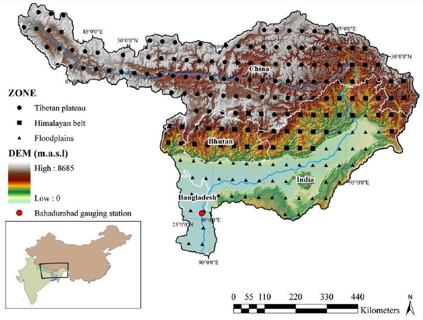
2. The Brahmaputra River Basin
2.1. Basin Characteristics
The river basin area is defined from the source on the Tibetan Plateau to the confluence with the Ganges
River after which it flows into the Bay of Bengal (Figure 1) (e.g. Immerzeel, 2008; Sarma, 2005). It
drains an approximate area of 530,000 km2 of which 50.5% lies in China, 33.6% in India, 8.1% in
Bangladesh and 7.8% in Bhutan (Immerzeel, 2008). Along its 2900 km course, it flows through diverse
environments. Immerzeel (2008) distinguished three distinct physiographic zones (percentage coverage
in brackets): the Tibetan Plateau (44.4%) with elevations of 3500 m above sea level and higher, the
Himalayan mountain belt (28.6%), and the floodplain (27.0%) with elevations of less than 100 m above
sea level.
 The Brahmaputra River originates from the Chema Yundung glacier in the Kailash range in South-
west Tibet at an elevation of 5300 m.a.s.l. (Sarma, 2005). On the cold and dry Tibetan Plateau, the river
is known as Tsangpo or Yarlung Zhanbo and flows an easterly course of 1625 km to the Himalayan belt
with a general slope of 1.63 m km/s3. The slope of the (Dihang) river increases greatly while passing
through the Himalayan Mountains: up to 16.8 m km/s3 (Figure 2).
 Through the steep mountains, it enters the Assam Valley. The Assam Valley is confined by the
Himalayas to the North and East and by the Meghalaya mountain reach to the South. The Himalayan
Mountains is geologically young and active region and therefore the amount of available sediment is
considerably high (Sarker et al., 2003). The valley receives large amounts of rainfall and has a warm
humid climate (see Section 2.2.); therefore, the intensity of weathering is also high. This results in high
amounts of transported sediment in the drainage network (Sarma, 2005). Upon entering the Assam Val-
ley however, the slope decreases rapidly. This congests the channels resulting in a highly braided
channel pattern (Ghosh & Dutta, 2012). After confluencing with two major tributaries further south, the
river is called Brahmaputra and flows a south and westerly course of about 900 km through its alluvial
plain. The slope consistently decreases over the Assam Valley down to 0.079 m km/s3 at the border

Figure 1. An overview of the Brahmaputra basin (Immerzeel, 2008).

 3

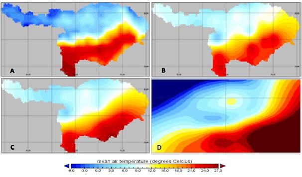
Figure 2. The longitudinal profile of the Brahmaputra River (modified after WAPCOS [1993] in: Sarma, 2005).

with Bangladesh (Sarma, 2005). The average width of the Brahmaputra riverbed varies between six and
18 km with few constraint reaches.
 The basin is characterised by high seasonal variability in flow, sediment transport and channel
configuration (Goswami, 1985). The integrated drainage network of the Brahmaputra and its tributaries
consist of various river dimensions and types. Especially in the floodplain, one can find straight, sinuous,
meandering, tortuous, braided, anastomosing, anabranching, reticulate and intermediate types. Subse-
quently, numerous palaeochannels exist in the region (Sarma, 2005).
 From the Bangladesh border, the Brahmaputra River (locally known as the Jamuna River) turns
southward with a reach of more than 300 km until the confluence with the Ganges River. The average
annual sediment transport through this part of the river is nearly 600 M ton/year (Sarker et al., 2003).
After the convergence, the river is known as the Padma River. Downstream, it merges with the Meghna
River after which it is named Lower Meghna River and continues into the Bay of Bengal.
 About 92.5% of the combined Ganges-Brahmaputra-Meghna basin area lies beyond the boundary
of Bangladesh (Mirza, 2003). On average, annual floods inundates 20.5% of Bangladesh (about 3.03
million ha) (Mirza, 2003). In exceptional years, floods may even inundate about 70% of the country, as
occurred during the floods of 1988 and 1998 (Ahmed & Mirza, 2000).

2.2. Meteorological Characteristics
Immerzeel (2008) published a chart with climate normals from 1961 to 1990 for the three physiographic
zones in the Brahmaputra basin (Figure 3A). The Tibetan Plateau is characterised by the coldest average
winter and summer temperature of -10℃ and 7℃, respectively. In the mountain belt, the average winter
temperature is around 2℃ while the summer temperature is around 15℃ on average. The lower Brah-
maputra river basin or floodplain has the highest average winter and summer temperatures: 17℃ and
27℃, respectively. In all zones, the temperature variation is largest during winter. Precipitation is con-
centrated during the monsoon from June to September for all distinguished regions (Figure 3B). The
wettest region is the floodplain and receives annual precipitation of 2354 mm (Immerzeel, 2008). How-
ever, the rain distribution is heavily affected by the large-scale orography prominent effects on
atmospheric flow patterns (Figure 4). Consequentially, annual rainfall is measured to be up to 5000 mm
(Sarma, 2005) or even higher (Nepal & Shrestha, 2015). Precise simulation of the spatial and temporal
behaviour of flow patterns in complex local topography is difficult to reflect in models due to the lack
of observational data (Beniston, 2003; Immerzeel, 2008)

 4

A B

Figure 4. Box-whisker plots with seasonal climate normals (1961–1990) of temperature (A) and precipitation (B) for the
Tibetan Plateau (TP), the Himalayan mountain belt (HB), and the floodplain (FP). Categorised for the spring (SP [=March,
April, May]), summer (SU [=June, July, August], autumn (AU [=September, October and November], and during the winter
(WI [=December, January, February]) (Immerzeel, 2008).

Figure 3. A normal annual isohyetal map of the Brahmaputra basin in the Assam Valley, India (unit in cm). (After WAPCOS
[1993] in: Sarma [2005]).

 Some 60–70% of the annual rainfall precipitates during the monsoon (Immerzeel, 2008; Mirza et
al., 2003), with a further 20–25% during the pre-monsoon from March through May (Nepal & Shrestha,
2015; Sarma, 2005). Clusters of successive rainy days with around 100 mm per day are standard during
the rainy seasons. Precipitation is characterised by an increasing trend from east to west along the Him-
alayas with its consequences for the dependent river basins (Immerzeel et al., 2009). The eastern part of
the Brahmaputra basin experiences less precipitation due to the Meghalaya Mountain reach inflicting
with large-scale wind directions during the monsoon (Figure 4). Additionally, snowmelt contributes
significantly to the total river discharge (Immerzeel et al., 2009).

 5

2.3. Hydrological Characteristics
Downstream water availability is sensitive to changes in snow and glacier extent (Immerzeel & Bier-
kens, 2012). Immerzeel et al. (2010) estimated that the discharge generated by snow and glacier melt in
the Brahmaputra basin is 27% of the total discharge generated in the basin.
 As mentioned above, precipitation occurs during the pre-monsoon and monsoon seasons with high
intensity and quantity. These events cause quick hydrological response in the form of flood waves
(Ghosh & Dutta, 2012). On average, the Brahmaputra River experiences four to five flood waves annu-
ally during the monsoon period (Datta & Singh 2004; Karmaker & Dutta 2010), causing floods in the
floodplain. About 40% of the fluvio-deltaic plain of the Brahmaputra River basin is prone to flooding
(Immerzeel, 2008). The physical factors contributing to this phenomenon include snow and glacier melt,
the El Niño Southern Oscillation (ENSO) induced conditions, loss of drainage capacity due to the silta-
tion of principal distributaries, backwater effect, unplanned infrastructure development, deforestation
and the synchronisation of flood peaks of the major rivers of the delta (Mirza et al., 2003). Mirza (2003)
compared three extreme floods (1987, 1988 and 1998) in Bangladesh and found intense monsoon pre-
cipitation was the primary cause of flooding.
 Bangladesh generally experiences four main types of floods (Mirza et al., 2003): flash, riverine,
rain and storm-surge. Eastern and northern areas of Bangladesh adjacent to its border with India are
vulnerable to flash floods. Rivers in these regions are characterised by sharp rises and high flow veloc-
ities resulting from storm events occurring in neighbouring India. Riverine floods occur when the major
rivers and their (dis-)tributaries flood due to increases in upstream river discharge. Rain floods are
caused by intense local rainfall of long duration in the monsoon months. Heavy pre-monsoon rainfall
causes local run-off to accumulate in topographic depressions. Local rain accumulates in ponds by rising
water levels in adjoining rivers. Coastal areas of Bangladesh, which consist of large estuaries, extensive
tidal flats, and low-lying offshore islands, are vulnerable to storm-surge floods, which occur during
cyclonic storms. Cyclonic storms usually occur during April–May and October–November.
 Floods are quite common during the (pre-) monsoon, while in the low-flow periods the river be-
comes a highly braided river with a large number of mid-channel and lateral bars (FAO, Aquastat, 2011).
Due to the braided nature of the river, measuring the discharge can be difficult and only possible at some
nodal points. At these constraint reaches, the bed level of the river generally undergoes aggradation and
degradation throughout the year. The average discharge of the Brahmaputra is measured to be approxi-
mately 20,000 m3/s (Datta & Singh, 2004; Immerzeel 2008). Sarma (2005) elaborates on the discharge
characteristics. The average monthly discharge is highest in July and lowest in February. The high flow
period that causes floods in the region starts in May and generally ends in the last weeks of October with
peak flows generally in the range of 60,000 to 70,000 m3/s with measured extreme peak discharges of
100,000 m3/s. From November to April, discharge is relatively low: 5000 to 6000 m3/s. Large variations
in discharge are noticed during a flood, with the maximum increase of about 17,000 m3/s in 24 hours
(June 7–8, 1990) and 24,000 m3/s in 48 hours (June 7–9, 1990) (Sarma, 2005). The maximum measured
discharge reduction over 24 hours was 12,000 m3/s at September 21–22, 1977.

 6

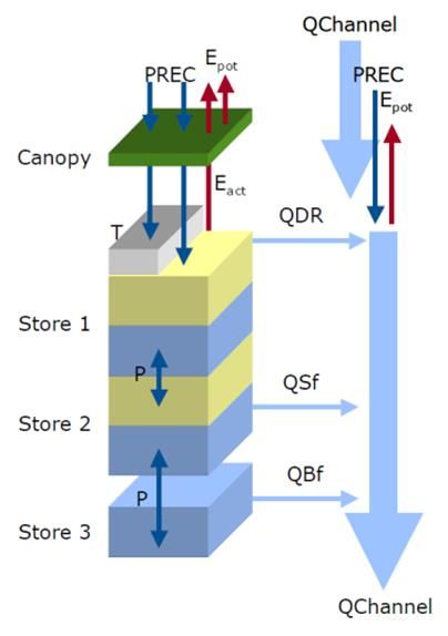
3. Research Methodology
In this study, different datasets were used: the WFDEI global water resources reanalysis forcing data
from the eartH2Observe project (E2O), and datasets based on locally observed data. The study will use
the PCR-GLOBWB model with a 5 arc minute spatial resolution (roughly 10×10 km) and a daily tem-
poral resolution. A spatial extent was created which encompasses the Brahmaputra River Basin
(Appendix A). The model was not calibrated for this basin.
 First, multiple forcing datasets were created from in-situ data from local stations using different
interpolation techniques. Precipitation and temperature input were compared using timeseries and maps.
Furthermore, an evaluation was done to investigate the influence of the different datasets in terms of
estimated discharge. The calculated discharge patterns were analysed with daily, monthly and mean-
monthly timeseries using the observed record at the Bahadurabad gauging station as reference. Addi-
tionally, verification metrics were used as indication of the performance of the model results. Finally,
different combinations of datasets and modifications of the E2O forcing data were investigated.

3.1. Hydrological Model: PCR-GLOBWB
In this study, the PCR-GLOBWB model was used. PCR-GLOBWB is a deterministic process-based
macro-scale lattice-based model describing global water balances of the terrestrial hydrology (Van Beek
et al., 2011; Van Beek & Bierkens, 2009). Similar to other global hydrological models, it is essentially
a “leaky-bucket” type of model (Bergström, 1995) applied on a cell-by-cell basis. The model is coded
in the dynamic scripting language PCRaster (Wesseling et al., 1996). The PCRaster Environmental
Modelling language is a high-level computer language that uses spatio-temporal operators with intrinsic
functionality for constructing spatio-temporal models. It enables a very efficient manipulation of raster-
based maps and has several built-in hydrological functions, such as accumulating and routing water and

Figure 5. Model concept of PCR-GLOBWB (Van Beek & Bierkens, 2009). The left-hand side represents the vertical structure
for the soil hydrology representing the canopy, soil column (stores 1 and 2), and the groundwater reservoir (store 3).
Precipitation (PREC) falls as rain if the temperature (T) is above 0°C or as snow if below 0°C. Snow accumulates on the
surface, and melt is temperature controlled. Vertical transport in the soil column is accounted for using percolation or
capillary rise (P). Potential evapotranspiration (Epot) is broken down into canopy transpiration and bare soil evaporation.
This is reduced to actual evapotranspiration (Eact) on the basis of soil moisture content. On the right-hand side, drainage
from the soil column to the river network occurs via direct runoff (QDR), interflow (QSf) or subsurface stormflow (QBf) as
total specific discharge from one cell to the subsequent grid cell. Drainage accumulates as discharge (QChannel) along the
drainage network and is subject to a direct gain or loss depending on the precipitation and potential evapotranspiration
acting on the open water surface.

 7

sediments over drainage networks. The model has been applied in various water resource balance stud-
ies, such as: calculating groundwater balances (Sutanudjaja et al., 2011; Wada et al., 2010),
consumptive use of surface water and groundwater resources (e.g. irrigation and industry) (De Graaf et
al., 2014; Gleeson et al., 2012; Wada et al., 2012, 2014), impact of climate change on irrigation (Wada
et al., 2011, 2013), river discharge (Sperna Weiland et al., 2010; Bierkens & Van Beek, 2009), and
impact of climate change on river discharge (Gain et al., 2011; Sperna Weiland et al., 2012). PCR-
GLOBWB calculates for every grid cell and for every time step the water storage in two vertically
stacked soil layers and for one underlying groundwater layer. A schematic overview is given in Figure
5. Water exchange between layers (capillary rise and percolation), and interaction between the top layer
and the atmosphere (snowmelt, evapotranspiration and rainfall) are calculated, as well as snow storage
and canopy interception. The process description presented in the remaining part of this Section is only
a short overview and only describes modelled processes related to this study. For more elaborate infor-
mation on the PCR-GLOBWB model, the author recommends Van Beek (2008), Van Beek and Bierkens
(2009), Van Beek et al. (2011), and Appendix A of Sutanudjaja et al. (2011).
 Climate forcing is applied at a daily resolution and assumed constant over the grid cell. Precipita-
tion falls as liquid or solid depending on the air temperature 2 m above the ground. Excess precipitation
either adds to the snow pack, adds to the liquid pore space in the snow pack, or infiltrates into the first
soil layer. Snow accumulation and melt are temperature driven and modelled according to the Hydrol-
ogiska Byråns Vattenbalansavdelning (HBV) snow model (Bergström, 1995). Precipitation can be
intercepted by the canopy (with finite storage capacity) and any intercepted water is subject to open
water evaporation. Excess precipitation is added to the snowpack if the air temperature is less than 0°C
( < 273 ). Above 0°C ( ≥ 273 ), precipitation and melt water are stored as liquid water in
the available pore space in the snow cover, or passed on to the first soil layer. The evapotranspiration
can be determined using either the Hamon method (Hamon et al., 1954) or the Penman-Monteith ap-
proach (Allen et al., 1998).
 Instead of using per-cell values for vegetation and soil types, the model recognizes sub-grid varia-
bility by taking into account a fractionized land type coverage, considering tall and short vegetation,
open water, and different soil types. Short vegetation extracts water from the top layer only, while tall
vegetation extracts water from both soil layers. Calculation of the fraction of saturated soil (indicated
with x) to assess direct runoff is based on the improved Arno scheme (Hageman & Gates, 2003) and the
digital elevation model with surface elevations of the 1×1 km Hydro1K dataset (USGS EROS Data
Center, 2006), and is derived by Van Beek and Bierkens (2009) as:

 − +1 (1)
 =1−( )
 − 

where , and indicate cell-averaged total soil moisture storage and maximum and min-
imum storage capacities, respectively, all in [m]. These parameters refer to the area in the cell not
specified as open water and are based on the FAO gridded soil map of the world (FAO, 1998). The
parameter [-] is a dimensionless shape factor that defines the distribution of soil water storage within
the cell and is calculated based on the distribution of maximum rooting depths. This in turn is derived
from the 1×1 km distribution of vegetation types from Global Land Cover Characteristics Database
(GLCC) (Hagemann, 2002; USGS EROS Data Center, 2002).

3.1.1. Surface Runoff
As mentioned above, precipitation and melt water are stored as liquid water in the available pore space
in the snow cover or passed on to the first soil layer. As such, the input to the first soil layer consists of
both non-intercepted precipitation and snowmelt. Melt water is first stored in the snow pack up to a
maximum storage capacity that is related to snow depth (in snow water equivalent) and an average snow
porosity. Water stored in the snow pack may refreeze or is subject to evaporation. Snowmelt in excess
of the snow water storage capacity is added to the precipitation. The sum of non-intercepted precipitation
and excess snowmelt infiltrates into the first soil layer if the soil is not saturated, while surface runoff
occurs if the soil is saturated.

 8

The actual water content corresponds to fractional saturation of the soil , see Eq. (1). Surface
runoff is related to cell-averaged moisture storage and net input . However, the input is
distributed first in the recipient grid cell (up to its maximum moisture storages) before new surface
runoff is distributed to the subsequent grid cell. The direct runoff is given by (Sutanudjaja et al., 2011;
Van Beek & Bierkens, 2009):

 0, if ( ) + ≤ 
 1 +1
 ∆ +1 ( )
 
 ( ) = ( ) − ∆ + ∆ [( ) − ( +1)∆ ] , if < ( ) + ≤ (2)
 ∆ 

 { ( ) − ∆ , if ( ) + > 

 with ∆ = − , and ∆ = − 

 Eq. (2) states that for a given , is only generated if + exceeds . The direct run-
off contributes to the total specific discharge discussed in Section 3.1.5. Soil column infiltrated water is
discussed in the next Section.

3.1.2. Vertical Water Exchange
As mentioned in Section 3.1.1., the sum of non-intercepted precipitation and excess snowmelt infiltrates
into the first soil layer if the soil is not saturated. The downward fluxes between the layers are equal
to the unsaturated hydraulic conductivity [LT/s3] of the top, Eq. (3) in Table 1. The unsaturated hy-
draulic conductivity depends on the degree of saturation . The is defined using the average soil
moisture content of the layer ̅, saturated soil moisture content and residual soil moisture (Eq.
[4]). These variables can be obtained by dividing , and by the thickness of the layer. The
maximum depth of the two upper soil layers are 0.3 and 1.2 m, respectively.
 If the relative degree of saturation of the top layer is smaller than that of the second layer ( 1 <
 2 ), an upward flux is generated (i.e. capillary rise) (Eq. [5]). This flux can be sustained by the soil
moisture deficit in the top layer and is proportional to the unsaturated hydraulic conductivity of the
second layer. For the groundwater layer, the upward flux is described in a similar way, except that (i)
the conductivity is the geometric mean of the conductivity of the second and the third layer, (ii) it only
occurs given the proximity of the water table, (iii) and that the resulting moisture content of the second
layer cannot rise above the field capacity ( 2 < ) (Van Beek & Bierkens, 2009): see Eq. (6). Here 5

 Table 1. A selection of equations used in the PCR-GLOBWB model for calculating vertical water exchange in the soil
 column (Van Beek & Bierkens, 2009). Symbols are explained below the table.
 Purpose Equation
 Downward fluxes 1→2 ( ) = 1 ( 1 ( ))
 between soil layers
 (3)
 2→3 ( ) = 2 ( 2 ( ))
 ( ̅ − )
 Degree of saturation = (4)
 ( − )
 Upward flux be- ( ) ∙ (1 − 1 ), if 1 < 2
 tween soil layers 2 2→1 ( ) = { 2 2 (5)
 0, if 1 ≥ 2
 and 1
 Upward flux be- √ ( ) ∙ (1 − 2 )0.5 5 , if 2 < and 3 > 0
 tween soil layers 3 3→2 ( ) = { ,3 2 2 (6)
 and 2 0, otherwise

 In Equation (3): and are the degree of saturation of layers 1 and 2, and indicates the unsaturated hydraulic
 ̅ is the average soil moisture content of the layer, is the saturated soil moisture
 conductivity [LT-1]. In Equation (4): 
 content, and is the residual soil moisture. In Equation (6): is the fraction of the grid cell with a groundwater depth
 within 5 m, the factor 0.5 is an estimate of the average capillary flux over the area fraction with a groundwater table
 within 5 m depth, and is the water storage in the groundwater layer.

 9

denotes the fraction of the grid cell with a groundwater depth within 5 m. It is thus assumed that capillary
rise is at maximum if the groundwater table is at the surface and 0 if it is 5 m or lower below the surface.
The factor ‘0.5’ is an estimate of the average capillary flux over the area fraction 5 with a groundwater
table within 5 m depth, and 3 is the water storage in the groundwater layer. Fluxes between the second
soil layer and the groundwater reservoir are mostly downward, except for areas with shallow ground-
water tables, where fluxes from the groundwater reservoir to the soil reservoir are possible during
periods of low soil moisture content.

3.1.3. Interflow
Interflow is modelled by a simplified approach based on the work of Sloan and Moore (1984) in which
the soil is idealized as a uniform, sloping slab with an average soil depth and inclination:

 ∆ ∆ 
 ( ) = (1 − ) ( − ∆ ) + ( ) ∙ [ 12 ( ) − 23 ( )],
 
 (7)
 ( − )
 with = ,
 2 ,2 tan( )

where is interflow per m slope width [L2T/s3], is the average slope length or drainage distance
[L], and ∆ is the discrete time step. Please note that 12 ( ) and 23 ( ) are the net fluxes between
indicated layers [LT/s3]. The parameter [T] is a characteristic response time with soil moisture
content at field capacity, is the saturated soil moisture content, ,2 is the saturated hydraulic conduc-
tivity in layer 2, and is the average slope between the cells. The average slope is determined from the
average of calculated slopes from Hydro1K dataset. Interflow is only calculated if the soil water content
in the second layer is above field capacity ( 2 ≥ ). Additionally, interflow is only calculated in moun-
tainous areas. For each grid cell, the fraction of soils with a soil depth smaller than 1.5 m is determined
and interflow from this fraction is calculated (Van Beek & Bierkens, 2009).

3.1.4. Baseflow
Besides surface runoff and interflow, the groundwater layer contributes to the total specific discharge
via baseflow . The groundwater reservoir is infinitely large; however, the active groundwater storage
is computed by assuming a linear relationship between storage and outflow (Eq. [8]):

 3 ( )
 ( ) = ,
 
 (8)
 ∆ 
 with 3 ( ) = (1 − ) 3 ( − ∆ ) + 23, ( ),
 
In this equation, means a reservoir coefficient which represent the average residence time of water in
the groundwater reservoir (Van Beek & Bierkens, 2009). 3 is the water storage in the groundwater
layer, ∆ is the discrete time step, and 23, ( ) is the net flux between layer 2 and 3 [LT/s3]. Van Beek
and Bierkens (2009) state that large-scale aquifer thickness information is lacking and is therefore un-
reliable. A constant aquifer thickness of 50 m is assumed.

3.1.5. Surface Water Accumulation and Routing
The total simulated specific runoff of a (local) cell [LT/s3] consists of surface runoff , interflow
 and baseflow (also appointed as QDR, QSf and QBf in Figure 5.) (Eq. [9] in Table 2). To acquire
the lateral specific discharge [L2T/s3] (i.e. drainage) (Eq. [11]), is used to determine the total
accumulated local runoff . This is determined by correcting for direct gain and loss by precipitation
 [LT/s3] and reference potential evapotranspiration 0, [LT/s3] over the open water fraction 
in the cell (sub-grid variability) (Eq. [10]). Open water evaporation occurs at the potential rate, with
different crop factors being applied to deep water (lakes and reservoirs) and shallow water (river
stretches) as suggested by Allen et al. (1998).

 10

Table 2. A selection of equations used in the PCR-GLOBWB model to determine the total lateral in-flow and accumulated
 discharge (Sutanudjaja et al., 2011; Van Beek & Bierkens, 2009). Symbols are explained below the table.
 Purpose Equation
 Total local runoff = + + (9)
 Direct inputs to = − 0, , (10)
 open water surface
 
 Lateral influx = = [(1 − ) + ] (11)
 
 3⁄
 2⁄ 5
 3
 Total discharge + 1 2 2 −1 ( ) = with 1 = ( ) and 2 = 3⁄5 (12)
 ℎ √ 
 2⁄
 3 √ 
 = ℎ → [substitute by ℎ ⁄ ] → ℎ
 
 3⁄
 Manning’s equation 2⁄ 5 (13)
 3⁄ 3
 = 5 ( )
 √ 

 In Equation (9): surface runoff , interflow and baseflow , all in [LT/s3]. In Equation (10): precipitation
 [LT/s3], reference potential evaporation over water , [LT/s3], and , [-] is the reference crop factor coeffi-
 cient assumed for water bodies. In Equation (11): total lateral flow [LT/s3], area of the cell [L2], length of the
 cell [L], and the open water fraction in the cell . In Equation (12): is the channel’s length [L], is Manning’s
 roughness coefficient [L5/6T/s3], is the wetted perimeter [L], and is the gradient. In Equation (13): is the hydraulic
 radius [L] and is the cross-sectional area of the channel [L2].
The specific discharge of each cell is then routed over a drainage network that defines flow to one of the
eight adjacent cells, according to the local drainage direction (LDD) method. This drainage network
either terminates at the ocean or at an inland sink in the case of land-locked basins (i.e. pits). River
discharge [L3T/s3] is calculated by accumulating and routing the total specific discharge to the sub-
sequent grid cell using the kinematic wave approximation of the Saint-Venant equation (Chow et al.,
1988) (Eq. [12]). Eq. (12) is a combination form of the momentum and continuity equation. A numerical
solution of the kinematic wave approximation is available as an internal function in PCRaster in which
the new discharge +1 at every point along the channel is calculated from the discharge from the pre-
vious time step. The coefficients 1 and 2 are determined using Manning’s equation (Eq. [13]) and are
passed over the LDD to the downstream cell. At the end of the time step, the calculated discharge is
used to retrieve the new stage, which is calculated under the assumption of a rectangular channel with
known channel depth and width. The new stage is passed to the next time step to estimate the wetted
perimeter for the calculation of 1 .

3.2. Data Description
3.2.1. Meteorological Forcing Data
3.2.1.1. WFDEI Dataset
The global forcing data used in this study is based on the WFDEI (WATCH Forcing Data methodology
applied to ERA-Interim data) product (Weedon et al., 2014). This dataset is based on its forbearer WFD
dataset (based on ERA-40 reanalysis data) (Uppala et al., 2005) created by the EU WATCH (Water and
Global Change) project to directly compare global hydrological model output of different models with
the range 1958 to 2001 (Haddeland et al., 2011; Harding et al., 2011, Harding & Warnaars, 2011). The
WFDEI dataset is comprised of both satellite and local data. The product consists of precipitation and
temperature data. This study uses a finer resolution version of the original WFDEI product. The WFDEI
data was downscaled in accordance to the method explained in Weedon et al. (2014). The downscaling
is based on the difference in elevation between the low-resolution digital elevation map (DEM) and a
high resolution DEM. The downscaled data is calculated for each cell of the high resolution DEM. The

 11

downscaled version has a resolution of 5 arc minutes, approximately 10×10 km. A practical improve-
ment of the WFDEI opposed to the WFD dataset, is that the dataset ranges from 1979 to 2012, which
allows for intercomparison with satellite data products (Weedon et al., 2014). This dataset is hereafter
indicated as E2O.

3.2.1.2. In-situ Datasets
The region is considered to have poor available data due to the non-data sharing policy between involved
countries. Only in recent years this has begun to change. The precipitation and temperature data (Ap-
pendix B) was acquired from two main sources. It was either made available by the Institute for Water
Modelling (IWM) or from the weather website Weather Underground (2015). This website is not scien-
tific and weather enthusiasts can link their personal weather stations to this website. The data has certain
shortcomings. For instance, many measurement stations do not have a complete record and some sta-
tions switch from daily to monthly data (or vice versa) in the record. It was opted to filter out unreliable
records and choose reliable stations such as airports and governmental buildings.
 The gathered temperature data has a combined period of 2004 to 2015. The number of stations with
precipitation data is higher. The observed precipitation data in Bangladesh have the best records with
the longest data range (1970-2014). The average percentage of missing values for temperature and pre-
cipitation are 1.85 ± 2.33% and 9.03 ± 7.03%, respectively. However, the stations in India and China
have substantial smaller time periods. These sets of records limit the range and analysis of the in-situ
dataset to a study period of four years: from 2009 up to 2014.
 In Figure 6 the distribution of the stations is shown. The density of the station network varies over
the basin significantly. The lower basin is well represented, especially considering the precipitation data.
However, a notable lack of stations is present in the upper part of the basin. The North-Western part of
the basin is not represented. The temperature data is more evenly distributed. These stations are regarded
as point data from which the data could be interpolated to create a spatial grid. This was done in ArcMAP
(Appendix C). Interpolating techniques applied in the study are Inverse Distance Weighting (IDW),
Spline, and Ordinary Kriging (OK) (Childs, 2004; Davis & Sampson, 1986).
 The IDW and Spline interpolation methods are deterministic interpolation methods. These methods
are directly based on the surrounding measured values. The IDW interpolation method determines cell
values using a linear-weighted combination of sample points. This method assumes that the variable
decreases in influence to an unknown location the further the known location is. The value assigned to
the unknown locations is determined by averaging values of specified amount of known locations or of

Figure 6. The Brahmaputra River basin with the locations of the stations with observed temperature (T) and precipitation
(P) data. Additionally, the location of the Bahadurabad gauging station is shown.

 12

values within a specified search radius. The weight of the values is a function of the distance of the
 known point to the unknown cell.
 The Spline interpolation technique estimates values to minimize surface curvature. Spline bends a
 surface that passes through the input locations while minimizing the curvature. It fits a mathematical
 relation to a specified number of known input locations. It is best used to estimate a variable that is
 smooth in nature, such as temperature and water table heights. However, it needs a sufficient number of
 known locations.
 As opposed to deterministic methods, OK is a geostatistical interpolation method. Geostatistical
 methods are based on statistical models for the relation among measured points. Given this fact, geosta-
 tistical methods, such as OK, are capable to produce a prediction surface as well as provide a measure
 of certainty of the predictions. OK assumes there is no trend in the data (i.e. no constant mean). OK
 assumes that the distance between known locations reflects a spatial correlation that can be used to
 explain variation in the surface. The kriging method applies a ‘best fit’ to a specified number of locations
 or to a number of locations in a specified search radius, to determine the output value of the unknown
 point. This is done by exploratory statistical analysis of the data, creation of a semi-variogram, and the
 creation of a surface. Kriging is most appropriate when a spatial correlation is present in the data.
 Generally, IDW is smoother than the Spline method and the Spline method is smoother than the
 OK method. Due to the fact that the known locations are not well distributed over the entire basin, the
 interpolation method is used for extrapolation as well. The three datasets distinguished will hereafter be
 identified as In-situ OK (IOK), In-situ Spline (ISpline), and In-situ IDW (IIDW).

 3.2.2. Observed Discharge Data
 Measured discharge data was taken from the Bahadurabad gauging station (25°18'N, 89°66'E), which is
 North of the confluence of the Brahmaputra River with the Ganges River (Figure 1 and Figure 6). The
 raw data was provided by the Bangladesh Water Development Board and the Institute for Water Mod-
 elling (BWDB, 2015) and consisted of two datasets. The datasets have an overlap period in 2012. The
 data represents daily and irregular timed 3-hourly rated discharge data (Appendix D).
 On aggregating the data, it was chosen to use the daily averaged discharge values. The mean devi-
 ation of average discharge of a single day to all 3-hourly measurements of that same day is 0.36%.
 Secondly, it was assumed that the datasets with overlap periods were better represented by the younger
 dataset when the difference was minor. Thus in the case of an overlap period in the 2012, dataset 2 was
 chosen over dataset 1. This resulted in an observed discharge dataset covering a time period of 1985 to
 2014 on a daily time scale (Figure 7).
 According to literature, the average discharge of the Brahmaputra is approximately 20,000 m3/s
 (Datta & Singh, 2004; Immerzeel 2008). The average discharge of this dataset is determined to be
 21,674.21 m3/s. The median discharge is 14,463.96 m3/s and the maximum value present in this database
 is 103,166.9 m3/s. However, there are gaps in the dataset and these gaps occur mostly during low flow
 conditions. An extreme example is displayed in Figure 8. The original dataset 1 and 2 are primarily used
 for flood forecasting by flood forecasting agencies (e.g. Flood Forecasting & Warning Centre of the
 Bangladesh Water Development Board) and research institutes (e.g. Institute for Water Modelling). As
 such, low flow periods are deemed less important. Therefore, it can be safely assumed that the actual
 average discharge would be lower. Of the completely aggregated dataset, 3.35% of days have missing
 discharge values. Over the last ten years, the percentage of missing values is 9.26%.
 110
 100
Rated Q * 103 [m3/s]

 90
 80
 70
 60
 50
 40
 30
 20
 10
 0
 1985 1987 1989 1991 1993 1995 1997 1999 2001 2003 2005 2007 2009 2011 2013
 Figure 7. The aggregated measured discharge over the period 1985-2014. The years with extreme flooding (1988, 1998,
 2004, 2007, and 2012) can clearly be observed.

 13

100

 90

 80

 70
Rated Q *103 [m3/s]

 60

 50

 40

 30

 20

 10

 0
 J F M A M J J A S O N D J F M A M J J A S O N
 Months in the years 2012 and 2013
Figure 8. An example of missing data in the observed discharge data at the Bahadurabad gauging station.

3.3. Combined and Modified Forcing Datasets
3.3.1. Bias-Correction Method
Different combinations of datasets and modifications of the E2O forcing data were investigated to im-
prove on the E2O dataset. Bias correction have been applied in many studies and in the studies of
Huffman et al. (1997) and Adler et al. (2000) effort was made to create a (multi-)satellite-gauge-model
to combine satellite and gauge station precipitation records to improve the prediction of precipitation in
sections not covered by gauging stations. The studies used different techniques, one using an additive
bias correction while the other study performed a ratio bias correction. Vila et al. (2009) combined these
techniques and opted for the minimum correction.
 To elaborate, the difference between additive bias correction and observed values, and the differ-
ence between ratio bias correction and observed values were calculated. The next step chooses the
minimum absolute correction of the two methods and adds to the former E2O value, and performs this
adjustment per cell and per timestep. The benefit of choosing the minimum forcing correction is that
this results in a minimum discharge change according to these two methods. A second advantage of
applying this method is that a correction value is created per cell and per timestep. The disadvantage of
using this approach is that the correction is applied to an already interpolated field. The correction fields
are created with conditional statements resulting in Boolean maps. Two example Boolean maps are
shown in Figure 9. The equations involved in this process are shown in Eq. (14):

 2 + ( ̅ − ̅ 2 ) = , if | − 2 | < | − 2 |
 2 , ={ ̅ (14)
 2 ( ) = , if | − 2 | ≥ | − 2 |
 ̅ 2 

in which 2 , is the new precipitation value, 2 is the former precipitation value of the E2O
forcing dataset, ̅ and ̅ 2 are the mean precipitation value of that particular cell of the indicated
dataset.
 Additionally, two regular ratio bias corrections to the E2O forcing were performed, one with 25%
and one with 40% more precipitation input.

 14

Figure 9. Two examples of the boolean condition map where red is 1 and blue is 0. These images are of the dates 26 and
27 September, 2011. If the statement is true (1), then the value of the additive bias correction was used, else the ratio bias
correction was used.

3.3.2. Forcing Data Combinations
A different approach to adjust the input forcing data is to acknowledge that the region consists of two
distinct physiographic and climatological regions (or even three [Immerzeel et al., 2008]). One being
the upper part of the basin and one being the lower part of the Brahmaputra River Basin. Thus, a crude
separation was made at latitude 28.50. The study was limited in creating straight separations along lati-
tude and longitude lines. This separation is based on the fact that the southern section is represented by
many stations contrary to the northern part (i). This makes for easy comparison between interpolated in-
situ forcing data and E2O forcing data input. The temperature distribution is characterised by a clear
separation along the Himalayan Mountains (ii) (Section 4.1.1). Mean difference in daily precipitation
can be regarded as two separate regions, based on the ratio (iii) and the linear difference (iv) (Section
4.1.2). The precipitation in the upper region is regarded to be generally overestimated using the IOK
dataset. Making the cut arguably slightly too high decreases the influence of the IOK precipitation in
the northern part (v). The modelled snow cover is left to the upper part (vi). This approach results in
four additional model runs: IOK precipitation data applied in the northern part and E2O precipitation
data in the southern part of the basin or vice versa, and E2O or IOK temperature data applied over the
whole basin.
 Additionally, interpolated in-situ and E2O forcing data were combined by using local precipitation
and global temperature, and vice versa. Furthermore, the difference in using Hamon or Penman-Mon-
teith (P-M) approach has been investigated. For this purpose, the E2O evapotranspiration (ET) data has
been applied in combination with both the interpolated in-situ forcing datasets and the E2O forcing data.

3.4. Verification Strategy
Model runs were performed with the E2O and interpolated in-situ forcing datasets. Temperature and
precipitation forcing analysis was done by comparing spatial patterns of time-averaged maps and field-
averaged daily values resulting in timeseries. The timing and amplitudes of minima and maxima in
timeseries were analysed. As well as directly comparing input forcing data with observed station data at
selected locations. Additionally, E2O forcing was compared with observed data at known locations.
Similarly, this approach was applied to the resultant evapotranspiration of the model runs.
 Furthermore, model estimated discharge was compared with observed discharge at the Baha-
durabad gauging station. The estimated discharge patterns were analysed for timing and discharge
values on daily, monthly and mean-monthly time scales. Additionally, the discharge was evaluated using
statistical verification metrics as indication of the performance of the model-estimated discharge com-
pared with the observed discharge (Helsel & Hirsch, 2002):
  The Nash–Sutcliffe model efficiency coefficient (NSE) (Moriasi et al., 2007; Nash & Sutcliffe,
 1970) is used to assess the predictive power of hydrological models. The efficiency can range
 from −∞ to 1. An efficiency of 1 corresponds to a perfect match of observed data and modelled
 discharge. An efficiency of zero means that the model results are as accurate as the mean of the
 observed data. An efficiency of less than zero occurs when the observed mean is a better pre-
 dictor than the model.

 15

 Pearson’s correlation (r) is a measure of degree of linear correlation between measured and
 estimated discharge values. A value of 1 indicates a perfect correlation while 0 means no cor-
 relation, a value of -1 indicates a negative correlation.
 The mean absolute error (MAE) indicates how close the predicted and observed values are.
 Relative small values indicates that the predicated and observed values are similar.
 The root-mean-squared error (RMSE) is used as a measure of accuracy between the predicted
 and observed value. A relative large value indicates a low accuracy, whereas a relative smaller
 value indicates a higher accuracy.
 The mean values of observed and estimated discharge were calculated.
 Additionally, the bias is the difference between the model estimated value and the observed
 value.

 16

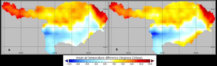
4. Results
4.1. Model Input Analysis
4.1.1. Temperature
Figure 10 displays the mean temperature over the whole study period. There is a large difference in
mean temperature over the basin. The upper part is colder than the lower part of the basin. ISpline
performs poorly in the areas over which it needs to extrapolate: it calculated mean temperature values
of -30°C in the North-Western area and +80°C in the South-Eastern area. Thus, the use of ISpline was
discontinued at an earlier stage. The results using IOK and IIDW forcing data are better and display a
similar pattern as the E2O forcing data model run.
 The temperature data of the E2O forcing dataset in the northern part of the basin is significantly
colder than the IOK and IIDW datasets. The mean temperature of E2O is around 3.25°C, while the
interpolated in-situ datasets have a mean value of 6.11°C. In the lower part of the basin, the E2O dataset
is only slightly warmer than the interpolated in-situ datasets.
 Figure 11 shows the mean temperature of the whole basin of every timestep. A significant bias can
be observed between the different forcing datasets. The difference between IOK and E2O is 3.17 ±
0.70°C and the difference between IIDW and E2O is 3.33 ± 0.75°C. However, as can be seen from
Figure 12, the distribution of mean temperature difference is not uniform over the whole basin. In the
lower part of the basin the temperature difference is between +1.0°C and -3.0°C, with the exception of
the area at approximately (27.0, 89.0): here the difference is up to -12.0°C. In the upper part of the basin,
the mean temperature difference is between +2.4°C and +14.5°C. There seems to be a large mean tem-
perature difference in the North and a smaller mean temperature difference in the South of the basin
between E2O forcing data and the interpolated in-situ forcing datasets.
 Two stations were chosen for a more detailed analysis: one in the upper basin: Lhasa (29.65, 91.14)
(Figure 13), and one in the lower part of the basin: Rangpur (25.76, 89.28) (Figure 14). The mean tem-
perature difference is generally present over the whole study period for both locations: the temperature
difference at the Rangpur station is small and E2O forcing values have a generally higher temperature
value than the in-situ datasets. However, the temperature difference at Lhasa is large and E2O forcing
values are significantly lower compared with interpolated in-situ forcing data.
 Considering the temperature spatial differences and distribution, it differs significantly over the
basin, however a distinction can be made between the upper and lower part of the basin.

Figure 10. Mean temperature value distribution over the Brahmaputra River Basin over the whole study period 2009-2012.
A – map based on the E2O forcing data input. B – map based on the interpolated station data using IDW. C – map based
on interpolated station data using OK. D – map based on interpolated station data using Spline (it was discontinued in an
earlier stage of the research).

 17