Detection of the cloud liquid water path horizontal inhomogeneity in a coastline area by means of ground-based microwave observations: feasibility ...
←
→
Page content transcription
If your browser does not render page correctly, please read the page content below
Atmos. Meas. Tech., 13, 4565–4587, 2020
https://doi.org/10.5194/amt-13-4565-2020
© Author(s) 2020. This work is distributed under
the Creative Commons Attribution 4.0 License.

Detection of the cloud liquid water path horizontal inhomogeneity
in a coastline area by means of ground-based microwave
observations: feasibility study
Vladimir S. Kostsov1 , Dmitry V. Ionov1 , and Anke Kniffka2
1 Department   of Atmospheric Physics, Faculty of Physics, Saint Petersburg State University, St Petersburg, Russia
2 Zentrum   für Medizin-Meteorologische Forschung, Deutscher Wetterdienst, Freiburg, Germany

Correspondence: Vladimir S. Kostsov (v.kostsov@spbu.ru)

Received: 20 February 2020 – Discussion started: 27 February 2020
Revised: 8 July 2020 – Accepted: 17 July 2020 – Published: 25 August 2020

Abstract. Improvement of cloud modelling for global and            are presented. The monthly averaged results are compared to
regional climate and weather studies requires comprehensive        the corresponding values derived from the satellite observa-
information on many cloud parameters. This information is          tions by the SEVIRI instrument and from the reanalysis data.
delivered by remote observations of clouds from ground-
based and space-borne platforms using different methods and
processing algorithms. Cloud liquid water path (LWP) is one
of the main obtained quantities. Previously, measurements          1   Introduction
of LWP by the SEVIRI (Spinning Enhanced Visible and In-
fraRed Imager) and AVHRR (Advanced Very High Resolu-               Improvement of global and regional climate and weather
tion Radiometer) satellite instruments provided evidence for       forecasting models requires comprehensive information on
the systematic differences between LWP values over land            atmospheric composition, physical and chemical processes,
and water areas in northern Europe. An attempt is made to          and in particular information on interactions between differ-
detect such differences by means of ground-based microwave         ent components of the climate system: the atmosphere, wa-
observations performed near the coastline of the Gulf of Fin-      ter areas, land surfaces, snow and ice cover, and the bio-
land in the vicinity of St Petersburg, Russia. The microwave       sphere. Boe and Terray (2014) analysed the role of soil–
radiometer (RPG-HATPRO, Radiometer Physics GmbH –                  atmosphere interactions, cloud–temperature interactions, and
Humidity And Temperature PROfiler), located 2.5 km from            land–sea warming contrast in European summer climate
the coastline, is functioning in the angular scanning mode         changes. High-resolution regional climate models were used
and is probing the air portions over land (at an elevation angle   (25 km) with a good realism of orography and coasts that
of 90◦ ) and over water (at seven elevation angles in the range    could help in reducing the biases in local climate existing in
4.8–30◦ ). The influence of the land–sea LWP difference on         low-resolution global climate model simulations. The study
the brightness temperature values in the 31.4 GHz spectral         by Fersch et al. (2020) has been devoted to the exchange
channel has been demonstrated, and the following features          of water, trace gases, and energy between the land surface
have been detected: (1) an interfering systematic signal is        and the atmospheric boundary layer. That study examined
present in the 31.4 GHz channel, which can be attributed to        the ability of the hydrologically enhanced version of the
the humidity horizontal gradient, (2) clouds over the opposite     Weather Research and Forecasting model (WRF-Hydro) to
shore of the Gulf of Finland mask the LWP gradient effect.         reproduce the regional water cycle by means of a two-way
Preliminary results of the retrieval of LWP over water by the      coupled approach and assessed the impact of hydrological
statistical regression method applied to the microwave mea-        coupling with respect to a traditional regional atmospheric
surements by HATPRO in the 31.4 and 22.24 GHz channels             model setting. One of the important parts of the climate sys-
                                                                   tem is cloud cover. Its variations significantly (and imme-

Published by Copernicus Publications on behalf of the European Geosciences Union.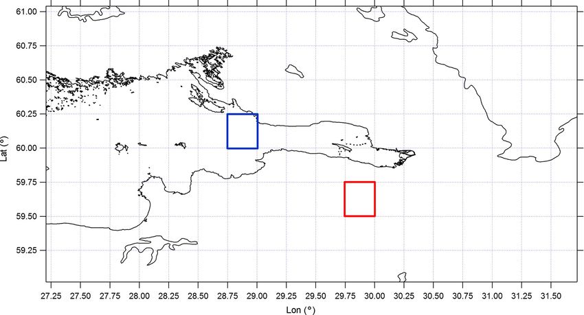
4566                                V. S. Kostsov et al.: Detection of the cloud liquid water path horizontal inhomogeneity

diately) alter the heat balance of the earth’s climate system      in the vicinity of St Petersburg (Russia) for the cold season
on an hourly timescale, but their effects are profound from        was noticeably lower than for the warm season. St Petersburg
seasonal through to decadal timescales; therefore, the phys-       is located at the estuary of the Neva river, which flows into
ical processes involving cloudiness–water-vapour–surface-          the Gulf of Finland. The magnitude of the land–sea differ-
temperature interactions need further investigation (Grois-        ence for mean LWP values obtained by SEVIRI in this area
man et al., 2000). Tang et al. (2012) have shown that the vari-    for the 2-year period of 2013–2014 was about 0.040 kg m−2 ,
ance of European summer temperature is partly explained            which was about 50 % relative to the mean value over land.
by changes in summer cloudiness. Europe has become less               In general, the investigation of cloud properties in the
cloudy (except north-eastern Europe) and the regions east of       coastal zones is an interesting and important task due to the
Europe have become cloudier in summer daytime. However,            presence of specific atmospheric processes, e.g. sea breezes,
the results obtained by Tang et al. (2012) suggest that the        which are able to generate clouds. A climatological study of
cloud cover is either the important local factor influencing       the impact of sea breezes on cloud types was done by Azorin-
the summer temperature changes in Europe or a major indi-          Molina et al. (2009a) for the area in the south-east of the
cator of these changes.                                            Iberian Peninsula (province of Alicante, Spain) and for the
   Clouds, as an important climate influencing factor, are de-     6-year period (2000–2005) based on cloud observations at a
scribed by a large number of parameters of microphysics and        synoptic station. The authors of the mentioned study empha-
macrophysics. Cloud liquid water path (LWP) is one of the          sise that their findings are site specific and should be simi-
main quantities, being a measure of the total mass of the liq-     lar to other coastal locations; however, cloud formation as-
uid water droplets in the atmosphere above a unit surface area     sociated with sea breezes is also influenced by geographi-
on the earth, given in units of kilograms per square metre         cal, physical, meteorological, hydrological, and oceanic fac-
(kg m−2 ). The information on LWP is delivered mainly by           tors. Therefore, there is a need for further research. The sea
remote observations of clouds from ground-based and space-         breeze effects were studied also on the basis of data derived
borne platforms using different methods and processing al-         from space-borne observations by the AVHRR instrument
gorithms. The principal space-borne techniques are based on        (Azorin-Molina et al., 2009b).
the derivation of LWP from measurements of atmospheric                The satellite instruments working in the visible and near-
self-emitted microwave (MW) radiation or from measure-             infrared ranges are very sensitive to the observational condi-
ments of the reflected sunlight in visible and the near-infrared   tions. There are specific requirements for SEVIRI observa-
ranges. The MW satellite sensors perform LWP measure-              tions: measurements are restricted just after sunrise and be-
ments during day and night but only over water areas since         fore sunset when the solar zenith angle (SZA) is too large
the emissivity of the land surface is highly variable. The ad-     (Roebeling et al., 2008; Kostsov et al., 2018b). Besides, the
vantage of the satellite instruments which register the re-        problem of the misinterpretation of measurements in winter
flected solar radiation in visible and near-infrared ranges is     over the snow-covered and ice-covered surfaces with high
the ability to make observations over water areas and the land     reflectance should be mentioned (Musial, 2014; Kostsov et
surface as well (but only in the daytime). Two instruments         al., 2019). Therefore, in the present study an attempt was
of this type are well known: SEVIRI (Spinning Enhanced             made to find a kind of supplement to satellite measurements
Visible and InfraRed Imager) and AVHRR (Advanced Very              in a coastal area in the form of detection of the land–sea
High Resolution Radiometer). The description of informa-           LWP gradients by means of ground-based microwave ob-
tion products delivered by these instruments and relevant to       servations. The concept of these measurements is straight-
cloud properties can be found in the papers by Stengel et          forward: a radiometer which is located close to a coastline
al. (2014, 2017).                                                  can probe the air portions over land and water surface if it
   Previously, measurements of LWP by the satellite instru-        works in the angular scanning mode at an appropriate di-
ments SEVIRI and AVHRR provided evidence for the dif-              rection. Microwave measurements can be carried out dur-
ferences between LWP values over land and water areas              ing all seasons, day and night, excluding rain and strong
in northern Europe. The data from the AVHRR instrument             snowfall conditions. Ground-based MW measurements char-
were used for compiling regional cloud climatology for the         acterise only the local-scale LWP distributions in the close
Scandinavian region (Karlsson, 2003). Analysis of this cli-        vicinity of the observational point, and this is their disad-
matology has shown that during spring and summer the               vantage when compared to satellite measurements. However,
cloud amount over land in this region is larger than the           they can provide important information on the diurnal cycle
cloud amount over the Baltic Sea and major lakes. Karls-           of LWP over land and water surface with high temporal res-
son (2003) explained this phenomenon by the stabilisation of       olution, and they also can be used for validation of satellite
near-surface layer of the troposphere over water bodies due        data on LWP obtained for the coastline area near the ground-
to air cooling by the cold fresh water from melting snow. This     based validation point. The RPG-HATPRO microwave ra-
explanation is in good agreement with the fact revealed later      diometer, which is functioning at the observational site of the
in the study by Kostsov et al. (2018b): the land–sea gradient      Faculty of Physics, Saint Petersburg State University (Rus-
of the mean LWP values detected by the SEVIRI instrument           sia), perfectly suits the requirements to the experiment aimed

Atmos. Meas. Tech., 13, 4565–4587, 2020                                             https://doi.org/10.5194/amt-13-4565-2020
V. S. Kostsov et al.: Detection of the cloud liquid water path horizontal inhomogeneity 4567
at LWP gradient detection. It is located at a distance of 2.5 km nal is 1 s. The sampling interval depends on operation mode.
from the coastline of the Gulf of Finland and performs angu- In the zenith-viewing mode, which is the main observational
lar scanning towards the Gulf of Finland every 20 min while mode, the sampling interval is about 1–2 s. Every 20 min,
doing routine observations. zenith measurements are interrupted and the angular scan-
The idea to use ground-based microwave radiometers in ning is done in the north-east direction with an azimuth of
the angular (elevation and azimuth) scanning mode for de- 24.7◦ .
tecting horizontal gradients and for plotting maps of atmo- Seven spectral channels located in the 0.5 cm oxygen ab-
spheric parameters is not new. The description of scanning sorption band (51.26, 52.28, 53.86, 54.94, 56.66, 57.30, and
radiometers and different methodologies, including the to- 58.00 GHz) provide information on the atmospheric temper-
mographic approach, can be found in a large number of ature profile, and seven channels located in the centre and the
articles, in particular by Crewell et al. (2001), Martin et wing of the 1.35 cm water vapour line (22.24, 23.04, 23.84,
al. (2006a, b), Westwater et al. (2004), Huang et al. (2010), 25.44, 26.24, 27.84, and 31.40 GHz) provide information on
Schween et al. (2011), Meunier et al. (2015), Stahli et the atmospheric humidity profile and cloud liquid water path.
al. (2011), and Marke et al. (2020). Zenith measurements are processed by the multi-parameter
To the extent of our knowledge, the studies devoted to retrieval algorithm based on the optimal estimation method
the detection of horizontal inhomogeneities of atmospheric (Kostsov, 2015a). Previously, the results of LWP retrievals
parameters from ground-based passive microwave measure- were validated, and the error analysis was made (Kostsov et
ments are not numerous, and ours is the first attempt to solve al., 2018a). Zenith and angular measurements in combina-
the specific problem relevant to the investigation of the LWP tion are also processed by the built-in quadratic regression re-
gradient in a coastline area. Therefore, we decided that it trieval algorithm developed by the instrument manufacturer.
would be reasonable to present the step-by-step analysis of Both optimal estimation and regression algorithms indepen-
the problem starting from the consideration of the forward dently provide the vertical profiles of temperature, absolute
problem and to demonstrate the complexity of the task that and relative humidity, integrated water vapour, and the cloud
faces us. We used the classical approach to the solution of the liquid water path. It is important to emphasise that the an-
inverse problem of atmospheric optics: analysis of the for- gular scans are used only for temperature retrievals in order
ward problem on the basis of simulations, analysis of mea- to improve the results at the boundary layer altitudes. This is
sured quantities for several test cases, tuning the retrieval al- a common procedure for radiometers of this type. The tem-
gorithm, processing the experimental data with the help of perature channels are optically thick, and as a result, the an-
this algorithm, and comparison of the results with the inde- gular measurements are not affected by horizontal inhomo-
pendent data. Although the concept of using angular mea- geneities of atmospheric parameters.
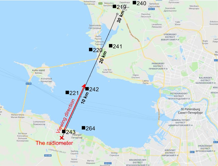
surements to characterise water vapour and liquid water path The location of the radiometer with respect to the coast-
gradients is feasible, its practical applications are very dif- line of the Gulf of Finland (Neva Bay) is shown in Fig. 1.
ficult due to the high variability of the liquid water in the The distance from the radiometer to the coastline is 2.5 km
clouds, the inhomogeneity of water vapour, etc. In addition, along the horizontal viewing direction. The horizontal line
we would like to emphasise that the experimental setup of the of sight crosses the opposite coastline of the Gulf of Fin-
HATPRO radiometer at our observational site was initially land at 18 km distance from the radiometer, and at the 22–
developed for improving temperature retrievals in the lower 26 km distance it passes over lake Sestroretsky Razliv. The
layers rather than for solving the problem of the LWP gradi- radiometer is located at about 25 km distance from the city
ent detection. However, we managed to apply these measure- centre (St Petersburg) and at about 50 km distance from the
ments to the task under consideration and received promising nearest radiosounding station (Voeikovo, WMO ID 26063).
results. The set of elevation angles of the line of sight of the mi-
crowave measurements is the following: 90, 30, 19.2, 14.4,
11.4, 8.4, 6.6, and 4.8◦ . The viewing geometry in the vertical
2 Description of the instrument, measurement plane is shown in Fig. 2. The radiometer is remotely prob-
geometry, and data processing algorithm ing the air portions over land at an elevation angle of 90◦
and over water areas at seven elevation angles in the range
2.1 General formulation of the problem 4.8–30◦ .
Different spectral channels have different responses to the
The 14-channel RPG-HATPRO radiometer (Radiometer spatial distributions of temperature, humidity, and cloud liq-
Physics GmbH – Humidity And Temperature PROfiler, https: uid water. The channels in the water vapour line and oxygen
//www.radiometer-physics.de/; last access: 30 May 2019) is band (at 22–28 and 51–58 GHz) are mainly influenced by
mounted on the top of a metal tower on the roof of the build- humidity and temperature distributions, while the channel in
ing of the Institute of Physics, Saint Petersburg State Univer- the so-called transparency window (31.40 GHz) provides in-
sity (59.88107◦ N, 29.82597◦ E; 56 m a.s.l.). The integration formation on LWP. In order to demonstrate that the “LWP
time of an instantaneous measurement of atmospheric sig- channel” is transparent enough in the entire atmospheric re-
https://doi.org/10.5194/amt-13-4565-2020 Atmos. Meas. Tech., 13, 4565–4587, 2020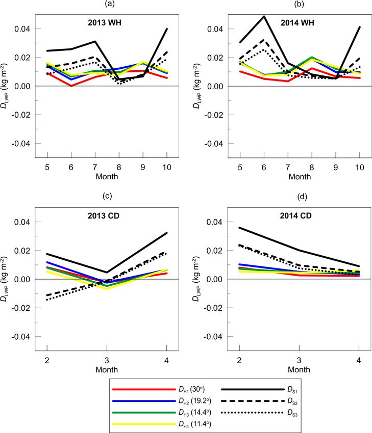
4568                                     V. S. Kostsov et al.: Detection of the cloud liquid water path horizontal inhomogeneity

                                                                           Figure 3. The 2D distribution of optical depth in the 31.4 GHz chan-
                                                                           nel as calculated from the radiometer location point (marked by the
                                                                           red cross). Overcast conditions; cloud base is 1 km; cloud top is
                                                                           2 km; LWP = 0.4 kg m−2 .

Figure 1. The location of the RPG-HATPRO radiometer and the                tained results lead to an important conclusion: clouds in the
viewing direction in the angular scanning mode. The black straight         layer 2–4 km over the opposite shore of the Gulf of Finland
line is the distance scale. Black squares (with numbers) show the          at about 20 km from the radiometer are detectable at small
position of the centres of the SEVIRI measurement pixels. Map data
                                                                           elevation angles (4.8–8.4◦ ). In the case that such clouds are
© 2019 Google.
                                                                           present, the detection of LWP land–sea gradient for clouds in
                                                                           the lower layers will become a rather complicated task.
                                                                              The measured atmospheric microwave radiation is regis-
                                                                           tered as a set of brightness temperature values, Tb , corre-
                                                                           sponding to observations at spectral channels with central
                                                                           frequencies ν and elevation angles α and will be designated
                                                                           as Tbm . Brightness temperature values which are calculated
                                                                           for any given set of atmospheric parameters will be desig-
                                                                           nated below as Tbc . Data processing was done according to
                                                                           the algorithm which is shown in Fig. 4. The set of Tbm is
                                                                           the basic input to the processing and analysis, but zenith and
Figure 2. The viewing geometry in the vertical plane. Position of          angular observations are treated separately. Zenith observa-
the radiometer is marked by the red cross. Coloured lines represent        tions at all 14 spectral channels are processed by the multi-
the lines of sight for different elevation angles (see the legend). Blue   parameter retrieval algorithm based on the optimal estima-
boxes designate the atmospheric layer, 0.3–5.5 km, over water areas
                                                                           tion approach. The obtained profiles of atmospheric param-
(see text).
                                                                           eters are then used for calculation of brightness temperature
                                                                           values corresponding to elevation angles of angular scans un-
                                                                           der the assumption of horizontal homogeneity of the atmo-
gion of interest, we calculated optical depth for this channel
                                                                           sphere. At the next step these calculated values are compared
along lines of sight corresponding to different elevation an-
                                                                           to corresponding measured values. The difference between
gles. The results are plotted in Fig. 3 as a 2D map. In order to
                                                                           measured and calculated brightness temperatures is taken as
model maximal absorption, as an input for the calculations,
                                                                           a main quantity for analysis:
we took the profiles of temperature and humidity which are
typical for warm and humid days in July in the St Peters-                  DTB (ν, α) = Tbc (ν, α) − Tbm (ν, α).                           (1)
burg region. The integrated water vapour was 31 kg m−2 . The
LWP of the modelled cloud was equal to 0.4 kg m−2 , which                  This quantity can be considered a sum of several terms:
is the maximal value for non-rainy clouds. Overcast condi-
tions were modelled; the cloud base and top were selected at               DTB (ν, α) = Dgrad (ν, α) + DTq (ν, α) + Derr (ν, α),           (2)
1 km and 2 km, respectively. One can see that even for this
extreme case the optical depth at 31.4 GHz does not exceed                 where Dgrad is the brightness temperature difference which
1.8 for the smallest elevation angle at a horizontal distance              is directly caused by the difference between LWP of a cloud
of 28 km from the radiometer, which is the opposite shore of               above the radiometer and LWP of a cloud observed at the el-
the Gulf of Finland and about 10 km inland. At the opposite                evation angle α. For simplicity, this term will be referred to
coastline, which is 18 km from the radiometer, the optical                 below as the LWP gradient signal. DTq is the brightness tem-
depth reaches a value of about 1 at its maximum. The ob-                   perature difference caused by the horizontal inhomogeneity

Atmos. Meas. Tech., 13, 4565–4587, 2020                                                      https://doi.org/10.5194/amt-13-4565-2020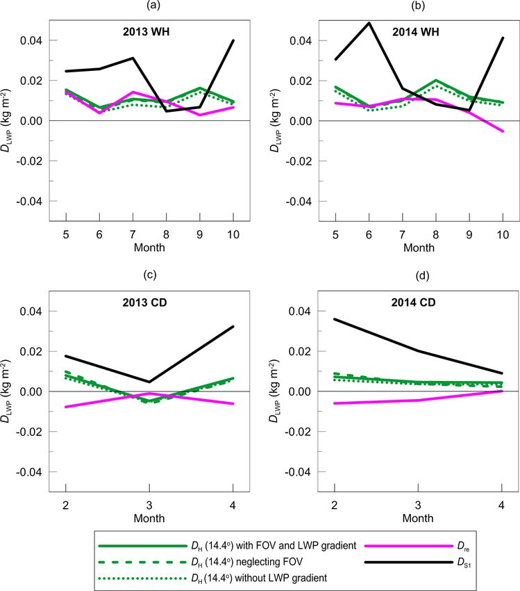
V. S. Kostsov et al.: Detection of the cloud liquid water path horizontal inhomogeneity                                         4569

of temperature and humidity. The term Derr is the interfer-
ing signal stipulated by errors and uncertainties of different
kinds. First, we point at the errors in retrieved profiles of at-
mospheric parameters which are used for calculation of Tbc
under the assumption of horizontal homogeneity. The contri-
bution of these errors to Derr needs more detailed explana-
tion. In order to make this explanation more evident, let us
consider the example case with a humidity profile error. Let
us imagine the situation when the error (the difference be-
tween the true and the retrieved humidity profile) is positive
in the lower layers of the troposphere and we know the true
profile. If we calculate Tbc for zenith direction using the true
and the retrieved profile, the difference between the obtained
Tbc values will be small and comparable to the random error
of microwave measurements, and the Tbc value will be very
close to the Tbm value. However, if we calculate Tbc for small
elevation angles using the “erroneous” profile and compare it
to the corresponding Tbm value, this difference can be notice-
ably higher due to the considerable increase in optical path
through the layers where the retrieved profile has errors. In
our example case, the result would be the overestimation of
Tbm by Tbc . Here, one important note should be made: the
retrieval errors for profiles have random and systematic com-       Figure 4. The algorithm for data processing and analysis.
ponents (the latter is caused mainly by a priori information
used for retrievals). As a result, the term Derr might consist
of both components also. The pointing error (elevation angle           For characterisation of a magnitude of the LWP gradient
error) can be another source of Derr , which is important for       signal, Dgrad , we present Fig. 5b where we modelled the at-
small elevation angles. Also, for small elevation angles, sur-      mospheric situation with the LWP land–sea difference. Ac-
face emission interference can take place through side lobes        cording to LWP measurements by the SEVIRI instrument in
of the antenna pattern. When considering small elevation an-        2013–2014 in the vicinity of St Petersburg, the mean LWP
gles, one should keep in mind the uncertainty of refraction         over the HATPRO radiometer site was 0.080 kg m−2 , and the
calculations stipulated by the uncertainty in the vertical and      mean LWP over Neva Bay was 0.040 kg m−2 (Kostsov et
horizontal distribution of atmospheric humidity.                    al., 2018b). We modelled 2D radiative transfer for ground-
   In order to give an impression of the origin of the LWP          based measurements using these values and disposing clouds
gradient signal, in Fig. 5a we present a simplified schematic       within 1–2 and 3–4 km altitude layers. The artificial cloud
picture of the MW radiation transfer from the atmosphere            with LWP = 0.080 kg m−2 was placed over the radiometer
to an instrument which makes an observation at some eleva-          location, and the artificial cloud with LWP = 0.040 kg m−2
tion angle. We consider two cases: a cloudy atmosphere and          was placed over the entire water area and over the opposite
a cloud-free atmosphere (temperature and humidity are as-           shore of the Gulf of Finland. Annual mean profiles of pres-
sumed to be the same). In the cloudy case, the radiation from       sure, temperature, and humidity for the St Petersburg region
the cold upper atmospheric layers is considerably absorbed          were taken as a necessary input for calculations, and the as-
by a cloud; at the same time, a cloud itself is a strong emitter    sumption of horizontal homogeneity of these parameters was
of radiation. As a result, an instrument registers the radiation    used. Figure 5b shows that, as expected, the 31.4 GHz chan-
which is formed mainly in warm atmospheric layers within            nel has the largest LWP gradient signal, which reaches 14–
and below a cloud. In the clear-sky case, an instrument can         16 K for the smallest elevation angle. The signals in the 22.24
“see” upper tropospheric layers which are cold and less dense       and 51.26 GHz channels, which are shown for comparison,
than the lower layers. Hence in a clear-sky case the measured       do not exceed 6 K. The signal at 51.26 GHz is nearly zero
brightness temperature is lower than it is in a cloudy case.        for the smallest elevation angle because of its high opacity
This reasoning is valid also in the case when clouds over a         when compared to other considered channels. For the 31.4
radiometer and over a water body have different LWP values:         and 22.24 GHz channels, the signal is higher when the cloud
the lower the LWP is, the weaker the emission by cloud and          is located within the 3–4 km layer than in the case of lower
absorption of downwelling radiation are. So the measured            cloud, but this difference is not large (about 2 K).
brightness temperature for clouds with low LWP values will
be smaller than for clouds with high LWP values.

https://doi.org/10.5194/amt-13-4565-2020                                              Atmos. Meas. Tech., 13, 4565–4587, 2020
4570                                 V. S. Kostsov et al.: Detection of the cloud liquid water path horizontal inhomogeneity

                                                                     Figure 6. Possible configurations of the observational geometry in
                                                                     the case of scattered clouds (a schematic illustration). Solid lines
                                                                     designate the line of sight (LOS) of the observations at various el-
                                                                     evation angles. Dashed lines show the field of view (FOV) of the
                                                                     radiometer.

                                                                     phasised that the average horizontal size of generated clouds
                                                                     was much smaller than the size of the water body under in-
                                                                     vestigation. While modelling the LWP values, we considered
                                                                     two situations: one with the existing LWP land–sea gradient
                                                                     and another without such a gradient. The mean LWP values
                                                                     for the first situation were the same as taken previously for
                                                                     overcast conditions: (0.08 and 0.04 kg m−2 for land and sea,
                                                                     respectively). For the second situation, the mean LWP value
                                                                     was taken as 0.08 kg m−2 everywhere. The number of gen-
                                                                     erated cases was about 165 000. Every instantaneous cloud
                                                                     spatial distribution was combined with one set of the me-
                                                                     teoparameter profiles (temperature, pressure, and humidity).
                                                                     For these meteoparameters, the assumption of horizontal ho-
                                                                     mogeneity was used. The sets of profiles were obtained in the
Figure 5. (a) A simplified scheme of the MW radiation trans-         course of 2 years of observations by the HATPRO radiome-
fer from the atmosphere to an instrument, illustrating the origin    ter (2013–2014) with the sampling interval of 2 min. As a re-
of the LWP gradient signal. (b) The LWP gradient signal, Dgrad ,     sult, we obtained a statistical ensemble which characterised
as a function of the elevation angle in three spectral channels.     all seasons.
LWPland = 0.080 kg m−2 and LWPsea = 0.040 kg m−2 . Solid and            The important issue which should be discussed with spe-
dashed lines correspond to the cloud located within 1–2 and 3–4 km   cial attention is the influence of the instrument field of view
layers, respectively.                                                (FOV) on the interpretation of the off-zenith measurements.
                                                                     The 22 and 31 GHz channels are optically transparent even
                                                                     for small elevation angles. If the vertical distributions of at-
2.2    Modelling of measurements in the atmosphere with              mospheric parameters within FOV at a certain distance from
       scattered clouds                                              the radiometer can be approximated by linear functions, the
                                                                     effect of FOV will be negligible. The situation can change
Figure 5b refers to an overcast atmospheric situation which          crucially in the case of scattered clouds, especially for small
is the simplest but idealised case for estimation of the magni-      clouds and small elevation angles. With a 3◦ FOV, the HAT-
tude of the LWP gradient effect in the measurement domain.           PRO radiometer will be sampling an air portion of about
In order to be closer to reality, we simulated the scattered         1 km vertical size at 20 km distance from the radiometer. Pos-
clouds over land and sea in the vicinity of the radiometer           sible configurations of the observational geometry in the case
using a Monte Carlo method. The observational plane (see             of scattered clouds are illustrated in Fig. 6. One can see that
Fig. 2) was extended and divided into cells (two rows, each          small clouds may appear entirely within FOV of the radiome-
row contained four cells of the 12 km × 3.25 km size) located        ter (as shown in Fig. 6 for the cloud over the opposite shore).
over the Gulf of Finland and two opposite shores. In each            Some clouds may be missed by observations due to their lo-
cell, the random-number generator produced the values of the         cation in between the lines of sight (LOSs) corresponding to
following cloud parameters: the vertical extent (0.3–2 km,           different elevation angles. Two or more scattered clouds may
uniform distribution), horizontal size (0.5–5 km, uniform dis-       fall into the FOV. Moreover, one cloud may be detected both
tribution), the cloud placement within a cell (uniform distri-       in zenith and off-zenith observations.
bution), and LWP (lognormal distribution). It should be em-

Atmos. Meas. Tech., 13, 4565–4587, 2020                                                https://doi.org/10.5194/amt-13-4565-2020
V. S. Kostsov et al.: Detection of the cloud liquid water path horizontal inhomogeneity 4571
Figure 8. The LWP gradient signal, Dgrad , as a function of the el-
evation angle at 31.4 GHz. Input data: the Monte Carlo model of
scattered clouds. Solid line (1) corresponds to the results obtained
when accounting for FOV; the dashed line (2) corresponds to the
results obtained when neglecting FOV.
relevant to the LWP gradient contribution. Therefore, we use
the same designation of this difference and show it in Fig. 8
Figure 7. Statistical distributions (in terms of relative frequency of
as a function of the elevation angle. One can see the dra-
occurrence R) of brightness temperatures at 31.4 GHz simulated for
matic contrast to the overcast case (see Fig. 5b). For scattered
four elevation angles and for two situations: one with existing LWP
land–sea gradient and another without such a gradient. Input data: clouds, there is no increase in the useful signal for smaller el-
the Monte Carlo model of scattered clouds. evation angles. On the contrary, the Dgrad values for elevation
angles 11.4 and 14.4◦ are lower than for the angles 19.5 and
30◦ . The sharp decrease of Dgrad at 11.4◦ is explained by the
Figure 6 demonstrates the large variety of atmospheric sit- influence of high LWP values of the clouds over the opposite
uations. Obviously, for scattered clouds it makes no sense shore of the water body.
to compare single zenith and off-zenith observations since In order to assess if the instrument FOV affects the magni-
the LWP gradient signal is a random value under such con- tude of the useful signal, we present in Fig. 8 the Dgrad values
ditions. It is evident that by taking into account not only which were calculated for an infinitely narrow beam width,
the spatial variability of clouds but also their temporal vari- i.e. neglecting FOV. The results show that there are no con-
ability we can speak about the LWP gradient component in siderable differences between the cases accounting for FOV
measurements only in terms of mean values obtained by av- and neglecting FOV. One should keep in mind that we com-
eraging over a large amount of data. Figure 7 presents the pare the results which were obtained by averaging of a very
statistical distributions of simulated brightness temperatures large number of individual simulated measurements.
at 31.4 GHz for four elevation angles. For each angle, two However, the effect of FOV exists, and it is illustrated by
situations are considered: one with existing LWP land–sea Fig. 9, which shows the statistical distribution of the differ-
gradient and another without such a gradient. The input data ence between the brightness temperature obtained when ne-
for radiative transfer calculations were the Monte Carlo sim- glecting FOV and the brightness temperature obtained when
ulations of scattered clouds described above. One can see accounting for FOV. We suggest that this difference is a mea-
from Fig. 7 that for all angles the distribution with gradient is sure which characterises in the best way the FOV influence
shifted towards smaller brightness temperature values when on the results of the interpretation of the off-zenith measure-
compared to the distribution without gradient; however, this ments. The effect of FOV shows itself in the form of addi-
effect is less pronounced for the elevation angle of 11.4◦ due tional measurement noise which has a systematic component
to the influence of the clouds over the opposite shore of the and a random component. The absolute value of the system-
water body. atic component (characterised by the mean value of the distri-
In order to estimate the component in measured quantity, bution) is less than 0.5 K for all four considered elevation an-
which is related to the LWP land–sea gradient effect, we gles, and this value can be considered negligible. No specific
analyse the difference between the mean values of Tb datasets dependence of the systematic component on the elevation an-
which were calculated for situations without and with the gle can be seen. In contrast, the random component, which is
gradient. This difference is equivalent to the Dgrad values characterised by the standard deviation, increases for smaller
shown in Fig. 5b and presents a measure of the useful signal elevation angles. The obtained values for the random compo-
https://doi.org/10.5194/amt-13-4565-2020 Atmos. Meas. Tech., 13, 4565–4587, 20204572 V. S. Kostsov et al.: Detection of the cloud liquid water path horizontal inhomogeneity
be used for processing measurements if the analysis is done
for averaged quantities.
There is still an emerging question: to what extent the sig-
nal relevant to horizontal inhomogeneity of LWP Dgrad inter-
feres with signals DTq and Derr . In order to obtain the most
realistic assessment of the magnitude of the latter signals, we
decided to analyse the results of angular scans which have
been made during several cloud-free days instead of com-
piling computer models of inhomogeneous temperature and
humidity fields suitable for the considered experiment. The
obtained estimates are presented in the next section.
3 Case study
Forward calculations and their comparisons with measure-
ments are the preliminary and essential steps before solving
inverse problems in many studies. Analysis in the measure-
ment domain can be especially useful when considering the
multi-parameter inverse problems which physically are ill
posed. The solution of such problems implies the application
of a priori information which can affect the result to a great
Figure 9. Statistical distributions (in terms of relative frequency of extent. Besides, in the case when multiple parameters are re-
occurrence R) of brightness temperature difference EFOV “TB ne- trieved simultaneously, their retrieval errors are coupled in a
glecting FOV minus TB accounting for FOV” at 31.4 GHz simu- complex way. These two factors can make the analysis in the
lated for four elevation angles. Input data: the Monte Carlo model domain of sought parameters difficult and ambiguous. There-
of scattered clouds. fore, we start with the analysis in the measurement domain
for better understanding of the useful and interfering signals.
Since clouds are atmospheric objects which are characterised
by extremely large spatial and temporal variability and since
nent can be used for the estimation of a minimal number of the experimental setup and geometry were not optimised for
individual measurements which should be sampled in order the considered task, the model simulations should be veri-
to suppress considerably the influence of FOV. For example, fied by comparison with experimental data. In addition, the
for a set consisting of about 600 individual measurements, theoretical prediction of the value of useful signal should be
the random component of the error due to neglecting FOV at compared to the experimental data.
the elevation angle 11.4◦ will be reduced to a value of about We analysed measurements which were made during
0.1 K. It means that, for the current experimental setup, aver- different atmospheric situations. These situations were se-
aging over the 10 d time period is enough for suppressing the lected on the basis of space-borne measurements of LWP
random error due to FOV. in the vicinity of St Petersburg by the SEVIRI instrument,
So, the described Monte Carlo simulations of clouds and which had been analysed earlier in the article by Kostsov
the brightness temperature calculations lead to several impor- et al. (2018b). In order to study the parallax effect of the
tant conclusions. First, we reiterate that for scattered clouds space-borne measurements, Kostsov et al. (2018b) compared
it makes no sense to compare single zenith and off-zenith ob- the results of LWP measurements made by SEVIRI for two
servations since the LWP gradient signal is a random value ground pixels: the one which is the nearest to the position of
under such conditions. Second, for averaged quantities, the the HATPRO radiometer and the other which is the neigh-
magnitude of the component of measured signal determined bouring pixel but located over the Gulf of Finland just to the
by the LWP land–sea gradient (useful signal) in the case of north of the radiometer. Measurements during 4 d were anal-
scattered clouds is rather small; therefore, one can expect dif- ysed (6 May, 6 June 2013, 5 and 11 October 2014) when
ficulties in detecting it, especially when taking into account large differences between LWP over land and sea were de-
the presence of a large number of interfering factors. Third, tected. In the present study, the consideration of only the two
the instrument FOV affects the results of the off-zenith mea- mentioned pixels is not sufficient. When the atmosphere is
surements in the case of scattered clouds by introducing addi- observed by the radiometer at small elevation angles, the air
tional noise. Its systematic component is small and averaging portions over the opposite shore of the Gulf of Finland will
over several hundred cases can minimise its random compo- make a contribution to measured radiance. Therefore, the dis-
nent. So the assumption of infinitely small beam width can tributions of clouds in pixels 241 and 219 (as shown in Fig. 1)
Atmos. Meas. Tech., 13, 4565–4587, 2020 https://doi.org/10.5194/amt-13-4565-2020V. S. Kostsov et al.: Detection of the cloud liquid water path horizontal inhomogeneity 4573
should be taken into account as well as in pixels 243 (the ra- of large uncertainty of the temperature profile and without
diometer location) and 242 (the Gulf of Finland). Analysing any information on the cloud vertical location. Based on the
the SEVIRI LWP data in four pixels, we tried to find the fol- abovementioned reasons, we consider the applied radiative
lowing long lasting atmospheric situations. transfer model accurate enough for making comparisons be-
tween measured and calculated brightness temperature val-
a. LWP is equal to zero in all four pixels; a cloud-free at- ues. Also, it is important to note that most of the cases which
mosphere is everywhere. This situation is best for as- were selected for analysis are characterised by clear-sky con-
sessing the DTq and Derr terms in Eq. (2). ditions over the water area; therefore, the cloud placement
error is absent for the off-zenith calculations.
b. A cloud-free atmosphere is in all pixels except one at
In order to quantify the accuracy of our forward calcula-
the radiometer location. This situation is best for assess-
tions, we present the values of the residual between mea-
ing the Dgrad term in Eq. (2) during the most favourable
sured brightness temperatures and the brightness tempera-
observational conditions (without background signal
tures which are calculated using the retrieved profiles of at-
formed by the clouds over the opposite shore of the Gulf
mospheric parameters for zenith observations. The rms resid-
of Finland).
ual RRMS and the mean residual Rmean are calculated for
c. A cloud-free atmosphere over water area and clouds every retrieval separately for seven humidity channels, for
over both shores of the Gulf of Finland. This is the worst seven temperature channels, and for all 14 spectral channels
case for detection of the land–sea LWP gradient since of the radiometer. These quantities are used for the data qual-
the effect can be masked by the background emission ity control during the routine observations: the results are fil-
from clouds over the opposite shore. tered out if RRMS for all 14 channels is larger than 1 K. The
large statistics comprising clear and cloudy conditions and
Prior to analysing the cases, we would like to make a all seasons show that RRMS and Rmean for humidity channels,
note concerning the accuracy of calculations of the bright- which are of primary interest in the present study, constitute
ness temperature difference. These calculations use tempera- on average 0.2 and 0.05 K, respectively. So, the Tb measure-
ture, humidity, and cloud liquid water profiles retrieved from ments are well reproduced. In order to gain confidence in
zenith observations as an input. It is well known that the the results relevant to the LWP inhomogeneity, we supposed
ground-based microwave method has rather poor spatial res- that it would be reasonable to take the absolute value of the
olution, which yields smoothed profiles and the very large threshold for the useful signal in DTB equal to 1 K, which is
uncertainty of the vertical placement of a cloud. This fact is 5 times larger than the typical RRMS value for humidity chan-
known, and it was quantified in a number of studies with the nels. The DTB values exceeding this threshold are mainly
help of the DOFS calculation (degrees of freedom for signal, related to the horizontal inhomogeneity of atmospheric pa-
which shows the number of independent pieces of informa- rameters. We took into account this threshold value when we
tion that can be extracted from observations). This essential plotted Figs. 6–10.
feature of the transfer of the downwelling microwave radi- In Fig. 10 the LWP values detected by SEVIRI in four
ation in the considered spectral region shows itself both in measurement pixels are displayed as a function of time for
the forward and inverse problems. The brightness tempera- the date 25 August 2013 (warm and humid season). Accord-
ture calculations for the zenith and off-zenith geometry are ingly, the values of brightness temperature difference DTB
equally insensitive to small-scale variations of the parameter for the set of elevation angles are plotted in the form of 2D
distributions along the line of sight. Therefore this smooth- time charts for two spectral channels. The colour scale con-
ing feature does not affect our calculations and relevant con- tains three parts. The pure yellow part corresponds to the
clusions. The current version of the retrieval setup assumes brightness temperature difference in the interval [−1; 1 K].
the placement of a cloud inside the 0.5–5.5 km altitude range An appearance of yellow colour in a 2D plot means that the
(low and medium clouds). Outside this range, the cloud liq- difference between measurement and model calculation is
uid water profile is constrained to zero values. The workabil- negligibly small for the corresponding combination of time
ity of this retrieval setup has been confirmed in the study de- and elevation angle. The red hue describes positive values of
voted to cross-validation of different methods of the LWP re- DTB , and the blue hue describes negative values. Figure 10
trieval (Kostsov et al., 2018a). For liquid water profile, DOFS refers to a cloud-free atmospheric situation as detected by
is less than 2, meaning there is only a small influence of the the SEVIRI instrument: the LWP values are all equal to zero
liquid water distribution on the results of the brightness tem- except for pixel 219 after 267.7 d (fractional days); however,
perature calculations. This fact indicates implicitly that the those values are less than 0.008 kg m−2 and can be consid-
placement of the cloud does not play a crucial role in for- ered negligibly small. Here and below we use UTC times and
ward calculations and in the solution of the inverse problem. fractional days. The day count starts on 1 December 2012 –
Also, a kind of proof for that is a wide use of regression al- the first day of selected datasets. Local noon is at 0.416 d
gorithms for joint IWV (integrated water vapour) and LWP (11:00 UTC). One can see that for the 31 GHz channel, DTB
retrieval from two-channel observations under the conditions values are close to zero for the elevation angle of 30◦ . For
https://doi.org/10.5194/amt-13-4565-2020 Atmos. Meas. Tech., 13, 4565–4587, 20204574 V. S. Kostsov et al.: Detection of the cloud liquid water path horizontal inhomogeneity
Figure 10. (a) The LWP in four SEVIRI pixels as a function of time. Figure 11. The same as Fig. 10 but for 2 March 2013.
(b, c) The difference between calculated and measured brightness
temperatures DTB (colour scale) as a function of time and elevation
angle for two spectral channels (2D plots, the channel frequency is example of a very small influence of the humidity variations
indicated in the plots); 25 August 2013. on DTq and Derr in the 31 GHz channel in a dry atmosphere.
The next plot (Fig. 12) corresponds to the case 1 May
2013, which is the combination of the abovementioned at-
smaller elevation angles, DTB becomes negative and its ab- mospheric situations A and B. It is very important to note
solute value increases. The map has only one specific signa- that it would be wrong to directly compare the signatures in
ture: at about 267.2 d the absolute value of negative DTB is the LWP plot (panel a) and in the 2D time charts for DTB
the largest reaching 14 and 26 K for 31 and 22 GHz chan- (panels b and c). The LWP of the SEVIRI retrieval is the re-
nels, respectively. In general, the brightness temperature dif- sult of averaging over the area of about 7 km × 7 km, while
ference for the 22 GHz channel is noticeably larger than for measurements by the HATPRO radiometer are very local. In
the 31 GHz channel. The reason for that is the larger optical contrast to the study (Kostsov et al., 2018b) in which only
thickness of the 22 GHz channel and higher sensitivity of this zenith observations with frequent data sampling were used,
channel to water vapour variations. we can not perform averaging of HATPRO measurements,
Figure 11 is similar to Fig. 10 and also refers to cloud-free because the sampling interval for angular scans (20 min) was
conditions but during cold and dry season (2 March 2013). In quite large for that. This fact should be taken into account
contrast to 25 August 2013, the results for the 31 GHz chan- when comparisons of panel (a) with panels (b) and (c) are
nel demonstrate a negligibly small difference between mea- made. One should not expect the precise agreement of signa-
sured and calculated brightness temperature within the whole tures on a timescale. Figure 12 demonstrates a large number
range of elevation angles. Some negative values appear occa- of positive values of DTB for the 31 GHz channel. The largest
sionally at elevation angles below 10◦ . For the 22 GHz chan- of them reach 4 K and correspond to the period of time when
nel, the difference between measured and calculated bright- SEVIRI detected clouds over the ground-based radiometer
ness temperature is negligibly small within the range of ele- (about 151.3–151.4 d). These positive values observed for all
vation angles 10–30◦ . For lower angles, DTB becomes neg- elevation angles are the LWP land–sea gradient signal, which
ative, but its absolute values are not large. This case is an is perfectly seen in the considered case despite the fact that it
Atmos. Meas. Tech., 13, 4565–4587, 2020 https://doi.org/10.5194/amt-13-4565-2020V. S. Kostsov et al.: Detection of the cloud liquid water path horizontal inhomogeneity 4575 Figure 12. The same as Fig. 10 but for 1 May 2013. Figure 13. The same as Fig. 10 but for 25 July 2013. is not large and does not exceed 4.5 K. For the cloud-free part over the radiometer, over the water area, and over the op- of the day (starting approximately from 151.45 d), we see the posite shore of the Gulf of Finland may be considered, to a appearance of negative DTB values with the largest absolute certain extent, random. This fact manifests itself as a mixture brightness temperature difference at small elevation angles. of positive and negative DTB . As a result, the LWP land–sea For the 22 GHz channel, negative DTB values were detected gradient, which obviously existed during the considered day at small elevation angles all-day long. according to SEVIRI observations, is completely masked due Let us consider the most interesting case, which is de- to the presence of cloudiness over the opposite shore of the scribed by Fig. 13. This is the case with heavy cloudiness Gulf of Finland. Starting from 236.6 d, clouds disappeared (LWP is reaching 0.3 kg m−2 ) over both shores of the Gulf everywhere and for this period the DTB 2D map is more ho- of Finland and clear conditions over the water area (25 July mogeneous. Similar to cloud-free situations during the warm 2013). We stress that we have information on the spatial and humid season described by Figs. 6 and 8, the DTB values distribution of clouds only from the SEVIRI observations. are predominantly negative for this period and the absolute Unfortunately, the ground-based measurements for 25 July difference of brightness temperatures is larger for small ele- 2013 are available starting only from 236.34 d; nevertheless, vation angles. the observational period is long enough for analysis. First, Figure 14 illustrates atmospheric conditions similar to we point at the large amplitude of the brightness tempera- Fig. 12, but the LWP values of the clouds over the radiometer ture difference: from −18 to 24 K. The reason for that is the are much larger (up to 0.25 kg m−2 ). At the same time there presence of clouds with high LWP. Second, we point at the are some clouds with much smaller LWP over the opposite mixture of positive and negative DTB values for the 31 GHz shore of the Gulf of Finland. We see that for the 31 GHz channel within the time period 236.34–236.6 d. As it was channel, positive DTB values prevail, showing evidence of already noted, the ground-based measurements are very lo- considerable LWP land–sea gradient even for small elevation cal, instantaneous, and not averaged. Therefore, if the cloud angles. For the 22 GHz channel, in contrast to Fig. 12, the distribution is fragmented, the disposition of separate clouds DTB values are also predominantly positive even for small https://doi.org/10.5194/amt-13-4565-2020 Atmos. Meas. Tech., 13, 4565–4587, 2020
4576                                V. S. Kostsov et al.: Detection of the cloud liquid water path horizontal inhomogeneity

                                                                        water body (the Gulf of Finland) was unknown: the SE-
                                                                        VIRI instrument provided averaged data on LWP, and
                                                                        there was no information on corresponding pressure,
                                                                        temperature, humidity profiles, or type of cloudiness.

                                                                     2. The effect of LWP land–sea gradient can be masked by
                                                                        the signal from clouds over the opposite shore of the
                                                                        Gulf of Finland.

                                                                     3. There is a systematic negative component of the bright-
                                                                        ness temperature difference DTB , which is clearly re-
                                                                        vealed under cloud-free conditions and can reach in the
                                                                        warm and humid season 20 K by its absolute value at
                                                                        small elevation angles. So far, we do not have enough
                                                                        information for accurate identification of the origin of
                                                                        this negative component. Pointing error (elevation angle
                                                                        systematic error) should have produced a signal which
                                                                        is constant in time, so that is not the case. The uncer-
                                                                        tainty of accounting for refraction is smaller by more
                                                                        than an order of magnitude. The interfering signal com-
                                                                        ing from the surface through side lobes of the antenna
                                                                        pattern is very unlikely to be the reason since the ef-
                                                                        fect depends on air humidity. So, only two explanations
                                                                        remain: the humidity horizontal gradient or the amplifi-
                                                                        cation of the systematic error of humidity retrieval when
                                                                        brightness temperatures are calculated for elevation an-
                                                                        gles other than 90◦ . The presence of the negative com-
                                                                        ponent of DTB can make it difficult to detect LWP land–
                                                                        sea gradients if these gradients are not very pronounced.
Figure 14. The same as Fig. 10 but for 30 May 2014.

                                                                 4    Statistical characteristics: seasonal features
elevation angles. The reason for that is the high signal orig-
inating from the clouds with large LWP. The “separation of       The main idea of this statistical analysis is to compare the
variables” in channels 22 and 31 GHz is obviously not perfect    monthly-mean values of two quantities: DLWP and DTB .
and that is why the 22 GHz channel is also sensitive to cloud    Here, DLWP is the difference between LWP obtained by SE-
liquid water, as the 31 GHz channel is sensitive to humidity     VIRI in pixels 243 (land, radiometer location) and 242 (sea,
distribution. As a result, in the considered case the positive   Gulf of Finland), and this quantity in our study is the ref-
signal of the LWP land–sea gradient Dgrad dominates in the       erence measure of the LWP land–sea gradient. DTB is the
22 GHz channel over the negative values of the sum of the        brightness temperature difference in the 31.4 GHz channel,
terms DTq and Derr (especially for small elevation angles).      which has been defined in Sect. 2 and contains the compo-
   Concluding this section, we can formulate the following       nent reflecting the LWP land–sea gradient.
statements:                                                         In order to minimise the influence of the interfering sys-
                                                                 tematic negative component of DTB attributed to the hu-
 1. As predicted, the LWP land–sea gradient (higher LWP          midity horizontal gradient, in statistical analysis we consider
    over land, lower LWP over water) is detectable and           only the elevation angles larger than 10◦ . The other advan-
    shows up as positive values of the difference between        tage of this limitation is the missing of most clouds over
    modelled and measured brightness temperatures of the         the opposite shore of the Gulf of Finland, over a second
    MW radiation. These positive values can be seen in the       small water area (Sestroretsky Razliv), and the land at about
    whole considered range of elevation angles (4.8–30◦ ).       28 km distance, because the atmospheric layers below ap-
    The experiment revealed that the magnitude of the use-       proximately 4 km are not scanned. For the sake of correct
    ful signal (Dgrad ) can vary from 2 to 24 K, depending       comparison of the ground-based and space-borne measure-
    on elevation angle and LWP land–sea difference (as it        ments, we omitted all HATPRO and SEVIRI measurements
    is provided by the SEVIRI satellite instrument). Obvi-       made for solar zenith angles (SZAs) larger than 72◦ since
    ously, thorough quantitative analysis is problematic due     the retrieval errors of the LWP measurements by SEVIRI
    to the fact that the true state of the atmosphere over the   strongly increase for large SZA. The SEVIRI and HATPRO

Atmos. Meas. Tech., 13, 4565–4587, 2020                                             https://doi.org/10.5194/amt-13-4565-2020
V. S. Kostsov et al.: Detection of the cloud liquid water path horizontal inhomogeneity 4577
datasets used for calculations of monthly-mean values con- values are as follows:
tained all available high-quality measurements. The elements
L
of these datasets were not synchronised, which means, for X
LWPn = akn Tkn + a(L+1)n , (3)
example, that when HATPRO did not produce data because
k=1
of rain or snow, the SEVIRI dataset might have had no gaps.
L L
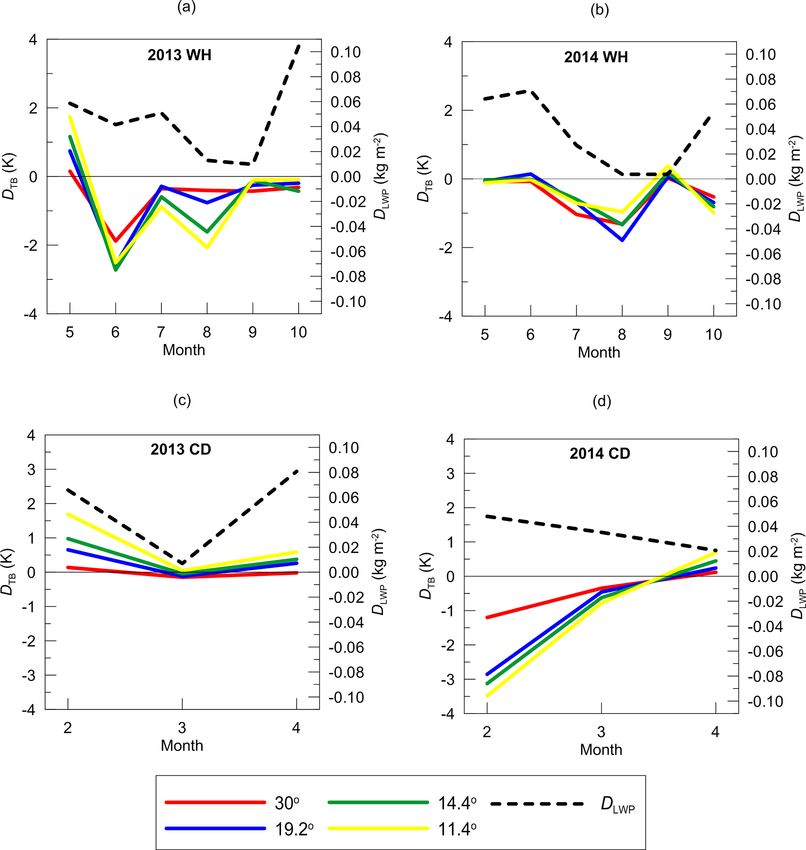
The monthly-mean values of DLWP and DTB are plotted X X
2
LWPn = bkn Tkn + b(L+k)n Tkn + b(2L+1)n , (4)
in Fig. 15 separately for 2013 and 2014 for warm and cold k=1 k=1
seasons. Prior to discussion of Fig. 15, two important notes
should be made. First, due to the presence of the system- where Eq. (3) refers to linear regression; Eq. (4) refers to
atic component (interfering signal) originating, as suggested, quadratic regression; n identifies the elevation angle of obser-
from the horizontal inhomogeneity of water vapour, atten- vations, in our case n = 0, . . ., 7 (zero refers to zenith view-
tion should be paid to the qualitative temporal behaviour of ing); a and b are the regression coefficients; index k identifies
DTB rather than to the specific values of this quantity. And the spectral channel; L is the total number of spectral chan-
second, one should account for the possible influence of sea- nels which are considered in the regression scheme; and T is
sonal variation of the interfering systematic component on the brightness temperature. In the present study, we used for
the temporal dependence of DTB . retrievals only two of seven spectral channels in the K-band:
As one can see from Fig. 15a, the LWP gradient detected 22.24 and 31.40 GHz, so L = 2 in Eqs. (3) and (4).
by the SEVIRI instrument during the warm and humid (WH) In the course of developing the retrieval algorithm, we
season has two maxima (in May–June and in October) and used two variants of training datasets. At first, we trained the
one minimum in August–September. Comparing DLWP and algorithm separately for each of the seasons and years and
DTB for the WH season, we note similar temporal behaviour considered only the overcast case with limited range of vari-
of these quantities within the time interval May–August. The ations of the cloud base and the cloud vertical extension. This
best agreement is observed for 2014. For 2013, the agree- approach appeared to be ineffectual and did not produce ro-
ment is not as good as in 2014 since the ground-based mea- bust results. It was found that extensive forward modelling of
surements demonstrate a profound minimum in June, which scattered clouds with highly variable parameters was neces-
is not present in the satellite measurements. For the cold and sary. Therefore, finally, training of the regression algorithms
dry (CD) season, there is a good agreement for the tempo- was performed on the basis of the Monte Carlo modelling of
ral behaviour of DLWP and DTB in 2013: maxima in Febru- the atmosphere with scattered clouds described in Sect. 2.2.
ary and April and a minimum in March. There is no agree- The complete training dataset included the values of LWP
ment for the CD season of 2014: the satellite data show calculated along the line of sight and converted to the LWP in
a slight decrease of the LWP gradient within time interval the vertical column. In the case of crossing several clouds by
February–April, while the ground-based data show an in- the line of sight, the LWPs from all these clouds were taken
crease. There is one interesting feature that should also be into account. The brightness temperatures at 22.24 GHz and
noted: the monthly-mean values of DTB for different eleva- 31.40 GHz were calculated by accounting for the instrument
tion angles are very close to each other for all seasons. How- FOV. This training dataset was used to derive the regression
ever, the variability of DTB in 2013 at small elevation angles coefficients. As a result, for each of the regression algorithms
(11 and 14◦ ) is higher than for large elevation angles (19.2 (linear or quadratic) of the LWP retrieval, we had at our dis-
and 30◦ ). posal eight sets of regression coefficients corresponding to
It should be reiterated that both water vapour and cloud eight elevation angles. Testing of the regression algorithms
liquid water affect the brightness temperature values which in the numerical experiments conducted for simulated over-
are registered in the so-called humidity channels (22– cast conditions and scattered clouds has shown that the algo-
31 GHz, K-band). When we analyse Fig. 15, we keep in rithms overestimate the true LWP for off-zenith observations
mind the interfering influence of atmospheric humidity on with the bias in the range 0.003–0.006 kg m−2 (for an eleva-
the values of DTB . In order to perform a separation of vari- tion angle of 60◦ ). The bias slightly increases for smaller el-
ables in our problem, we need to abandon the analysis of the evation angles. For zenith observations, the bias is negligibly
quantities in the measurement domain (brightness tempera- small. So, we can make the conclusion that the algorithms
tures) and start the analysis in the domain of sought param- can not overestimate the LWP gradient if it is detected while
eters, which in our case are LWP and IWV (integrated wa- processing field measurements.
ter vapour). The simplest and most commonly used method After applying the regression algorithms to the brightness
to solve the inverse problem of the LWP and IWV retrieval temperature values measured at different elevation angles,
from microwave observations in the K-band of microwave we could estimate the land–sea LWP difference as obtained
spectra is the application of regression algorithms – linear from ground-based MW observations using the following
or quadratic. Both algorithms have advantages and disadvan- formula:
tages; therefore we decided to apply both of them and to
compare the results. The regression formulae for the LWP DHn = LWP0 − LWPn , (5)
https://doi.org/10.5194/amt-13-4565-2020 Atmos. Meas. Tech., 13, 4565–4587, 2020You can also read