Characterizing uncertainty in the hydraulic parameters of oil sands mine reclamation covers and its influence on water balance predictions ...
←
→
Page content transcription
If your browser does not render page correctly, please read the page content below
Hydrol. Earth Syst. Sci., 24, 735–759, 2020
https://doi.org/10.5194/hess-24-735-2020
© Author(s) 2020. This work is distributed under
the Creative Commons Attribution 4.0 License.

Characterizing uncertainty in the hydraulic parameters of
oil sands mine reclamation covers and its influence on
water balance predictions
M. Shahabul Alam1 , S. Lee Barbour1,2 , and Mingbin Huang1,3
1 Department   of Civil, Geological and Environmental Engineering, University of Saskatchewan,
Saskatoon, SK, S7N 5A9, Canada
2 Global Institute for Water Security, University of Saskatchewan, Saskatoon, SK, S7N 3H5, Canada
3 Center for Excellence in Quaternary Science and Global Change, Chinese Academy of Sciences, Xian 710061, China

Correspondence: M. Shahabul Alam (msa181@usask.ca)

Received: 7 April 2019 – Discussion started: 12 June 2019
Revised: 9 October 2019 – Accepted: 18 December 2019 – Published: 18 February 2020

Abstract. One technique to evaluate the performance of              and parameter uncertainty have a similar influence on the
oil sands reclamation covers is through the simulation of           variability in net percolation.
long-term water balance using calibrated soil–vegetation–
atmosphere transfer models. Conventional practice has been
to derive a single set of optimized hydraulic parameters
through inverse modelling (IM) based on short-term ( < 5–           1   Introduction
10 years) monitoring datasets. This approach is unable to
characterize the impact of variability in the cover proper-         The hydraulic parameters of reclamation soil covers on oil
ties. This study utilizes IM to optimize the hydraulic proper-      sands mine waste have most commonly been characterized
ties for 12 soil cover designs, replicated in triplicate, at Syn-   by calibrating water dynamics models against a single profile
crude’s Aurora North mine site. The hydraulic parameters for        of field-monitored water content and suction. In many cases,
three soil types (peat cover soil, coarse-textured subsoil, and     this has been undertaken by deriving a single set of optimized
lean oil sand substrate) were optimized at each monitoring          parameter values from inverse modelling (IM) of short-term
site from 2013 to 2016. The resulting 155 optimized param-          (5–10 years) monitoring data (Alam et al., 2017; Boese,
eter values were used to define distributions for each param-       2003; Huang et al., 2015, 2011a, b, c; Keshta et al., 2009;
eter/soil type, while the progressive Latin hypercube sam-          Price et al., 2010; Qualizza et al., 2004). Devito et al. (2012)
pling (PLHS) method was used to sample parameter values             recommend that model calibration be focused on seasonal
randomly from the optimized parameter distributions. Water          and inter-annual climate variability (e.g., wet or dry) and also
balance models with the sampled parameter sets were used            take into account spatial variations in water movement within
to evaluate variations in the maximum sustainable leaf area         a spatially heterogeneous landscape. The current modelling
index (LAI) for five illustrative covers and quantify uncer-        approach that attempts to determine a single set of “best fit”
tainty associated with long-term water balance components           properties based on IM of a single monitoring station is un-
and LAI values. Overall, the PLHS method was able to bet-           able to characterize the spatial or temporal variability within
ter capture broader variability in the water balance compo-         the hydraulic properties of the cover soil and underlying mine
nents than a discrete interval sampling method. The results         waste. Quantifying spatial and temporal variability would be
also highlight that climate variability dominates the simu-         of value when assessing the expected long-term performance
lated variability in actual evapotranspiration and that climate     of reclaimed oil sands closure landscapes. However, spatial
                                                                    and temporal variability (i.e., uncertainty) in model parame-
                                                                    ters is not conventionally quantified or incorporated into the

Published by Copernicus Publications on behalf of the European Geosciences Union.
736 M. S. Alam et al.: Uncertainty in the hydraulic parameters of mine reclamation covers
soil–vegetation–atmosphere transfer (SVAT) models used to sociated with watershed response to climate variability
simulate long-term cover performance. (Benke et al., 2008). Various Monte Carlo (MC)-based ap-
The focus of this study is characterization of the uncer- proaches (e.g., generalized likelihood uncertainty estima-
tainty in the hydraulic parameters of reclamation soil covers tion (GLUE; Beven and Binley, 1992), the Metropolis algo-
over oil sands mining waste and the impact of this uncer- rithm, and Monte Carlo Markov chain (MCMC; Metropo-
tainty on predictions of the long-term water balance for these lis et al., 1953)) can be used to sample parameters ran-
sites. The two key measures of success for oil sands mine domly from the posterior distributions of the optimized pa-
reclamation are the water balance components of actual eva- rameters. Given that MC-based sampling strategies can be
potranspiration (AET) and net percolation (NP). AET quan- computationally expensive and sometimes unaffordable for
tifies the ability of the cover to support re-vegetation, while computationally demanding models, other sampling strate-
NP quantifies recharge into the underlying mine waste and gies have been developed and improved over the last several
the concomitant impact on water and contaminant release to decades. Of these, Latin hypercube sampling (LHS; McKay
downgradient surface water bodies. et al., 1979) has been most commonly used for uncertainty
The temporal variability of hydraulic parameters for these and sensitivity analysis in the field of water and environmen-
cover soils has been characterized by both direct testing and tal modelling (Hossain et al., 2006; Gong et al., 2015; Hig-
IM. Temporal variability in hydraulic conductivity (Ks ) was don et al., 2013; Sheikholeslami and Razavi, 2017). The LHS
measured in reclamation covers over saline–sodic overbur- approach offers a sampling strategy that can significantly re-
den at Syncrude’s Mildred Lake mine by Meiers et al. (2011), duce the sample size without compromising the accuracy of
and a similar evolution in Ks was also obtained through IM uncertainty estimation compared to the MC sampling ap-
by Huang et al. (2015). Such observed temporal variability proach (Iman and Conover, 1980; Iman and Helton, 1988;
was assumed to be the result of changes in density and pore- McKay et al., 1979). However, a major drawback of tradi-
size distribution of reclamation soils as a result of freeze– tional LHS- and MC-based sampling strategies is that the en-
thaw or wet–dry cycles and vegetation establishment. Spa- tire sample set is generated together and, unfortunately, an
tial variability would be expected to occur in reclamation appropriate sample size is not known a priori. An appropri-
covers because of variations in soil texture, cover construc- ate sample size here refers to a sufficiently large number of
tion/placement conditions, topography, or vegetation estab- sampled parameters so as to achieve convergence towards a
lishment. For example, Huang et al. (2016) characterized the common mean and standard deviation (SD) of the parame-
spatial variability of Ks using air-permeability testing of cov- ters, as well as the mean and SD of major components of the
ers. water balance (e.g., AET and NP).
More recently, IM has been undertaken on multiple mon- The appropriate sample size for each parameter can be de-
itoring sets collected over multiple years to evaluate the im- termined using a convergence criterion in the case of LHS;
pact of parameter variability on the predicted long-term per- however, the whole sample size is discarded if the conver-
formance of reclamation covers (Alam et al., 2017; Huang gence criteria fail, and a new set of simulations must be con-
et al., 2017; OKC, 2017). Recently, Alam et al. (2017) and ducted with a larger sample size to achieve convergence. To
Alam et al. (2018b) undertook a preliminary evaluation of overcome this computationally demanding approach, a new,
the impact of variability in the hydraulic properties of recla- efficient, and sequential sampling strategy called progres-
mation covers on the long-term water balance of oil sands sive Latin hypercube sampling (PLHS; Sheikholeslami and
reclamation covers. In that study, IM using HYDRUS-1D Razavi, 2017) can be used. In PLHS, the sample size is di-
was undertaken for four different reclamation covers (repli- vided into a series of smaller subsets (in place of the sin-
cated in triplicate) over 3 monitoring years to characterize gle sample set used for LHS), and each subset is added pro-
the water retention and hydraulic conductivity of the covers. gressively to sequentially grow the sample size. This can be
The calibrated (optimized) parameters showed that parame- summarized as follows: (i) each smaller subset forms a Latin
ter variability could be linked to both spatial and temporal hypercube, (ii) the progressively added subsets form a Latin
variability, but was dominated by spatial variability. A key hypercube, and (iii) the entire sampled parameter set (con-
limitation of this previous study was that the variability in sists of all smaller subsets) also forms a Latin hypercube.
the hydraulic properties was represented only by discrete val- The details on LHS and PLHS are provided in Appendix A.
ues (i.e., the mean value of the parameter as well as upper The two key advantages of the PLHS method over other
and lower bounding values) without a full statistically based sampling methods (e.g., MC) are as follows: (i) it achieves
characterization of the parameter variability. The value of a given convergence criterion with a smaller number of sam-
full statistical description of variability in characterizing the ples (i.e., smaller sample size) and (ii) it allows for sequen-
uncertainty in the predicted water balance of the covers under tial sampling without having to discard the whole sample size
a prescribed, future, climate variability was unknown. when convergence criteria are not attained.
The use of soil hydraulic parameters with spatial and/or The key research question of this study is as follows: what
temporal variability instead of a single parameter set can is the influence of soil hydraulic parameter uncertainty on
provide more information about prediction uncertainty as- the long-term cover performance of the reclamation covers
Hydrol. Earth Syst. Sci., 24, 735–759, 2020 www.hydrol-earth-syst-sci.net/24/735/2020/M. S. Alam et al.: Uncertainty in the hydraulic parameters of mine reclamation covers 737
in northern Alberta, Canada? This question led us to the fol- (by weight), while the general texture of the mineral com-
lowing study objectives: (i) identify the most efficient way ponent of LFH was sand (about 92 % by mass). The cover
to characterize distributions of the optimized hydraulic pa- soil was underlain by different selected coarse-textured sub-
rameters from a physically based water balance model for an soils salvaged from different locations (i.e., depositional en-
oil sands reclamation cover in northern Alberta, Canada, and vironments) and depths within the mine site (Soil Classifi-
(ii) quantify relative uncertainty from various sources asso- cation Working Group, 1998). In general, the subsoil texture
ciated with the long-term water balance of the reclamation is sand (92 %–95 % by mass). The bottom layer was con-
covers. structed using LOS overburden materials that were overlain
These objectives will be met by undertaking IM of mul- by cover soil and subsoil layers. The LOS materials consist
tiple monitoring sets (multiple monitoring sites in multiple of loamy sand to sandy loam with an oil content of 0.1 % to
years) to develop a statistical distribution of parameter vari- 7.7 % (NorthWind Land Resources Inc., 2013). Overall, the
ability. These distributions will be primarily utilized within a LOS comprises a range of different oil contents and particle
PLHS-based sampling approach to predict variability in the sizes compared to the cover soil and subsoil materials. All of
expected performance of the covers over the long term based the 13 treatment covers (which include two sub-categories of
on SVAT modelling. Comparisons will determine how these TRT 12) were included in this study.
predictions differ if either a discrete or continuous distribu- Particle size distribution (PSD) analyses of the cover soil
tion function is used to characterize material variability. To (LFH and peat), subsoil, and LOS were performed by a com-
the best of our knowledge, this more rigorous approach to mercial laboratory (OKC, 2009) in November of 2009 based
evaluating the long-term performance of soil covers has not on ASTM standard testing method D422 (ASTM, 1998). The
been conducted in general or specifically applied to the eval- ASTM D422 method is based on the assumption that the par-
uation of oil sands reclamation covers. ticles are spherical in shape, so the PSD for peat may not be
representative. The PSDs for the LFH and peat cover soils,
coarse-textured subsoil, and LOS are presented in Fig. 2.
2 Materials and methods The PSDs for the subsoils are the most variable, being sal-
vaged from different depths and depositional environments
2.1 Study sites and reclamation covers located on the Aurora North mine site. For the purposes of
the IM, the peat and LFH cover soils were ultimately com-
This study used soil monitoring data and meteorological data bined into a single group, as were different salvaged subsoils
collected from the Aurora Soil Capping Study (ASCS), lo- and LOS overburden materials. Combining the soil layers
cated at the Aurora North Mine of Syncrude Canada Ltd. in this manner produces additional variability within each
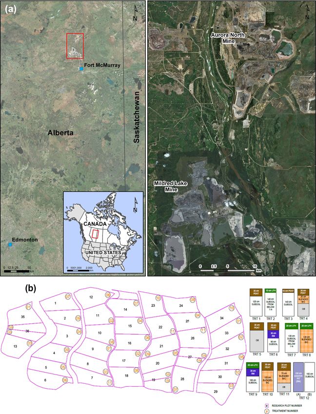
(SCL) in Alberta, Canada (Fig. 1a). The ASCS is comprised grouping; however, it ensures the maximum number of ob-
of a series of 12 alternate, 1 ha covers, replicated in trip- servations are utilized to capture the variability associated
licate, and placed over a lean oil sands (LOS) overburden with each layer of the soil reclamation covers. According
dump. The primary purpose of the different cover designs to Syncrude Canada Ltd., in the final cover design, the top
was to compare the performance of alternate materials and layer might be either peat/LFH or a combination of the two,
cover thicknesses in supporting vegetation and net percola- and the distributions of parameters for these two materials
tion (OKC, 2017). The layouts of the 12 covers (replicated) together seem reasonable for use in the illustrative covers for
are shown in Fig. 1b and are designated by a treatment num- long-term simulation of water balance components. There-
ber (i.e., TRT no.), with each treatment having 3 replicate fore, the PLHS method was used to randomly sample from
cells for a total of 36 cells in the ASCS that were randomly the distributions of the two materials grouped together.
placed across the watershed.
All the treatment covers within the ASCS were con- 2.2 Field monitoring data
structed in 2012 using three distinct soil layers, including
cover soil, subsoil, and LOS. The cover soil utilized in the A climate monitoring station (Aurora Met) was established in
treatment covers was either salvaged peat or LFH material. 2012 to measure precipitation, air temperature, wind speed,
The Soil Classification Working Group (1998) in Canada de- net radiation, and relative humidity at the study site. The
fined LFH as “organic soil horizons (L, F, H) developed pri- precipitation (rainfall and snow depth), air temperature, rel-
marily from the accumulation of leaves, twigs and woody ative humidity, wind speed, and net radiation were measured
materials, with or without a minor component of mosses, daily and/or hourly using automated methods of measure-
that are normally associated with upland forest soils with ment. The measurement instruments included a Texas Elec-
imperfect drainage or drier”. The L, F, and H horizons are tronics TE525 tipping bucket (rain) and SR50 sonic ranging
characterized by the accumulation of original organic mat- sensor (snow depth) for precipitation, a CS HMP45C sen-
ter, partially decomposed organic matter, and decomposed sor for air temperature and relative humidity, a RM Young
organic matter, respectively. The peat was predominantly or- 05103AP anemometer for wind speed, and a KIPP & Zo-
ganic material with a total organic carbon of about 17 % nen NRLife net radiometer (OKC, 2017). Each treatment cell
www.hydrol-earth-syst-sci.net/24/735/2020/ Hydrol. Earth Syst. Sci., 24, 735–759, 2020738 M. S. Alam et al.: Uncertainty in the hydraulic parameters of mine reclamation covers Figure 1. (a) Location map of Aurora North Mine of Syncrude Canada Ltd. (map sources: Esri, DigitalGlobe, GeoEye, Earthstar, Geo- graphics, CNES/Airbus DS, USDA, USGS, Aerogrid, IGN, and the GIS User Community) and (b) soil cover design treatments (TRT) at ASCS (adapted from OKC, 2017). LOS overburden (OB) underlies all treatments, even though treatments with less than 150 cm total soil cap thickness only show OB. Hydrol. Earth Syst. Sci., 24, 735–759, 2020 www.hydrol-earth-syst-sci.net/24/735/2020/
M. S. Alam et al.: Uncertainty in the hydraulic parameters of mine reclamation covers                                                   739

Figure 2. Particle size distribution (PSD) for (a) LFH, (b) peat, (c) subsoil, and (d) LOS materials for the treatment covers (OKC, 2009).
The lines in the subplots show PSDs for different samples collected from the LFH, peat, subsoil, and LOS layers, respectively.

also had a soil monitoring location where volumetric water             1D, potential evapotranspiration (PET) is calculated from
content, temperature, and suction were measured at multiple            climatic conditions using the Penman–Monteith equation
depths (typically every 10 cm) within the treatment covers             (Brutsaert, 1982). It is then apportioned into potential evap-
and the underlying LOS. The volumetric water content was               oration (PE) and potential transpiration (PT) based on a pre-
measured using Campbell Scientific CS616 time domain re-               scribed leaf area index (LAI) value. The actual evapora-
flectometers (TDRs), and the soil temperature and suction              tion (AE) from the ground surface is calculated from the
were measured using CS229 suction sensors (OKC, 2017).                 pressure head gradient between the top two nodes and hy-
The monitoring data utilized in this study were collected              draulic conductivity with two limiting conditions: (1) AE
from 2013 to 2016.                                                     must be less than PE and (2) the calculated water pres-
                                                                       sure at the top node must be in the range from 0 kPa to a
2.3   Parameter estimation using inverse modelling                     maximum suction equivalent to the atmospheric water va-
                                                                       por pressure. Actual transpiration (AT) is calculated by dis-
The meteorological and soil monitoring data were used to               tributing PT over a prescribed rooting zone where root wa-
calibrate a physically based SVAT model for each treatment             ter uptake is limited by water stress, as calculated by a root
cell based on IM. This provided a set of optimized soil hy-            water uptake model (Feddes et al., 1974). The root wa-
draulic parameter values for the cover soil (LFH or peat), the         ter uptake parameters were obtained from previous stud-
subsoil, and the LOS. These parameters were interpreted to             ies on the oil sands mine reclamation covers by Huang et
define spatial (cell to cell variation) and temporal (year-to-         al. (2011a, 2015, 2017). The Feddes model parameters were
year variation) variability in the saturated hydraulic conduc-         set as P0 = 0 kPa; P2H = −5000 kPa; P2L = −8000 kPa;
tivity (Ks ) and water retention curves (WRCs). The Mualem             P3 = −19 000 kPa; r2H = 0.5 cm d−1 ; and r2L = 0.1 cm d−1
tortuosity parameter was set to 0.5 and was not optimized as           for all models as obtained from the preliminary study on the
the goal was to only optimize a limited set of key parameters.         same sites by Huang et al. (2017).
This is denoted by l in HYDRUS-1D and defined as the pore-                HYDRUS-1D embeds an IM method into the numerical
connectivity parameter in the hydraulic conductivity function          solution of Richard’s equation. The IM method uses the
as estimated by Mualem (1976) to be approximately 0.5 as an            Marquardt–Levenberg gradient-based approach (Simunek et
average for many soils.                                                al., 2013) in which values of the five individual model param-
   IM is a mathematical approach that estimates unknown                eters (i.e., θr , θs , α, n, Ks ) are varied for each material until a
causes (e.g., model parameters) using observed variables               combination of the parameters is found that provides an opti-
(e.g., water content and/or pressure heads) during a historical        mal fit to the observed variation in a specific observation (i.e.,
period by iteratively solving the governing equation (Hop-             volumetric water content) (Hopmans et al., 2002). The first
mans et al., 2002). The governing equation (i.e., Richard’s            four parameters (θr , θs , α, n) are known as van Genuchten
equation) for water flow in unsaturated soil was solved us-            (VG) parameters (van Genuchten, 1980) and are used to de-
ing HYDRUS-1D (Simunek et al., 2013). In HYDRUS-

www.hydrol-earth-syst-sci.net/24/735/2020/                                              Hydrol. Earth Syst. Sci., 24, 735–759, 2020
740 M. S. Alam et al.: Uncertainty in the hydraulic parameters of mine reclamation covers
scribe the volumetric water content function (i.e., water con- the optimized and measured key parameter values was as-
tent vs. suction). Ks is the saturated hydraulic conductivity of sumed to be an indirect validation of the inverse modelling
the soil. A closed form solution then estimates the hydraulic approach used in this study, which can be used for further
conductivity function (i.e., K vs. suction) from the VG pa- sampling based on PLHS with a certain level of confidence.
rameters and Ks . How well these individual parameters are
estimated determines the overall accuracy of parameter esti- 2.4 Discretization of the model domain
mation. Details of IM used in HYDRUS-1D can be found in
Simunek et al. (2013). The simulated model domain used in HYDRUS-1D had a
In this study, the embedded IM method in HYDRUS-1D maximum height of 2.50 m with a minimum of 1.00 m of
was used to simulate volumetric water content by optimiz- LOS overlain by the various soil profiles (Fig. 1b). The vari-
ing the soil hydraulic parameters until the simulated water ous soil cover designs (TRT) are summarized in Fig. 1b. Note
content matched the measured values at various depths and the following cover construction: Treatments 2 and 7–9 used
times. To optimize the parameters, an initial value as well as LFH as the cover soil layer; Treatments 4, 8, and 10–11 were
a search range defined by an upper and lower limit of each constructed using blended B/C horizons as the subsoil; and
parameter were specified. The initial parameter values with Treatments 6, 9, and 12a were constructed using a Bm as the
their lower and upper limits for TRT 10 (cell no. 23 in year subsoil layer. Figure 1b also demonstrates the choice of two
2013) are shown in Table 1 for the peat and subsoil recla- depths (0.10 and 0.30 m) for the peat, two depths (0.10 and
mation materials as well as for the LOS substrate. To con- 0.20 m) for the LFH, and various depths for the subsoil recla-
duct IM in this study, the ranges of initial parameter values mation materials. The spatial discretization used for all of the
were estimated from the measured particle size distributions model domains was 1 cm and the time step was 86.4 s.
(PSDs) and bulk density using the Arya–Paris model (Arya
2.5 Initial and boundary conditions
et al., 1999). The WRCs for each PSD from peat/LFH, sub-
soil, and LOS were estimated using the equations presented Only the days in which the treatment covers were unfrozen
in the Arya–Paris model, and the RETC least-square opti- were simulated in the IM. Snowmelt infiltration and drainage
mization program (van Genuchten et al., 1991) was used to following ground thaw were assumed to be complete prior to
fit the VG–Mualem equation to the estimated WRC from the the start of the simulation. As a consequence, any snowmelt-
Arya–Paris model to estimate the VG parameters (θr , θs , α, induced change in the soil water storage was already incor-
n). The Kozeny–Carman equation (Kozeny 1927; Carman porated into the water content profiles from the first unfrozen
1938, 1956) was used to estimate Ks values from the PSDs, day (i.e., soil temperature > 0 ◦ C). The measured volumet-
as it is one of the most widely used and accepted methods ric water content profile of the first unfrozen day was set as
(Huang et al., 2011a; Mathan et al., 1995). The estimation of the initial condition, while a unit gradient (i.e., gravity gra-
parameters using these methods helps to constrain the initial dient) was set as the lower boundary condition of the model
parameter ranges in the inverse modelling. In addition to the domain. The SVAT parameters (e.g., climate and vegetation
Ayra–Paris model, the initial range of θs can also be approx- characteristics) were used as the upper boundary condition.
imated from the measured water content data for the covers,
where the maximum water content values are observed at the 2.6 Vegetation and root distribution
depths of 5–10 cm. After setting up the initial range of pa-
rameter values based on the above methods, the inverse mod- Maximum LAI values for each treatment cover were esti-
elling is repeated with different initial values. Once there is mated from measurements by Bockstette (2017) and pho-
no significant change in the θr and θs parameters and the ob- tographs taken on site by OKC (2017). The estimated LAI
jective function (i.e., sum of least squares), these parameters values varied from 0.2 at TRT 5 to 1.5 at TRT 2, TRT 7, and
are assumed to be optimized and kept fixed in the subsequent TRT 8. Huang et al. (2017) found that the temporal varia-
IM for the remaining parameters. Step by step the least sen- tion obtained with IM for similar sites was relatively minor
sitive parameters are kept fixed, thereby reducing the number compared to the spatial variability in the cover properties.
of parameters to be optimized by IM. Reducing the number Examining the photographs revealed that the sites were ini-
of parameters, constraining the range of initial parameter val- tially bare and developed a vegetative cover over the first few
ues, and repeating the IM with initial parameter values were years. Although the covers were planted with one of three
done as recommended by Hopmans et al. (2002). However, tree species (i.e., trembling aspen, jack pine, white spruce) or
details of all these steps are not included in this paper, only a mix thereof, the dominant early establishment vegetation
referenced to Hopmans et al. (2002), for the brevity of the pa- during the study period (2013–2016) was understory vege-
per. It is important to note that the purpose of this manuscript tation species (not trees). The understory development (i.e.,
was not to focus on IM techniques, but rather to highlight density and species) was variable, depending on the treat-
how reasonably optimized parameter sets can resemble the ment cover soil materials (i.e., peat or LFH; Jones, 2016).
distribution of the measured key parameter (i.e., Ks ) and rep- Due to the early dominance of understory species, the LAI
resent the parameter variability. This comparison between was assumed to be relatively constant over the study pe-
Hydrol. Earth Syst. Sci., 24, 735–759, 2020 www.hydrol-earth-syst-sci.net/24/735/2020/M. S. Alam et al.: Uncertainty in the hydraulic parameters of mine reclamation covers 741
Table 1. Initial value and lower and upper limits of the five soil hydraulic parameters for TRT 10 (cell no. 23 in 2013) used in the inverse
modelling to optimize parameters for peat, subsoil, and LOS.
Parameter value
θr (m3 m−3 ) ∗ θs (m3 m−3 ) α (m−1 ) n∗ (–) log (Ks ) (m s−1 )
Peat
Initial value 0.0160 0.610 4.50 1.50 −4.53
Lower limit 0 0.461 2.50 1.20 0
Upper limit 0.0900 0.700 6.80 2.30 −3.64
Subsoil
Initial value −2.22 0.361 2.50 0.310 −4.62
Lower limit 0 0.261 2.50 0.310 0.0
Upper limit −1.05 0.500 4.80 0.360 −3.64
LOS
Initial value 0.0900 0.368 4.50 1.74 −6.14
Lower limit 0 0.328 3.00 1.55 0
Upper limit 0.0900 0.450 6.50 1.83 −4.94
∗ The logarithmic (log 10) values are shown for θ and n parameters of the subsoil layer.
r
riod (i.e., 4 years). The seasonal distribution of LAI adopted subsoil variations could be grouped together for the simplifi-
for the simulations was the same as that used by Huang et cation of long-term water balance simulations.
al. (2015): (a) a linear rise in the spring from zero to a max- The Kolmogorov–Smirnov (K–S) test was used to ver-
imum value, (b) maximum in the summer, and (c) a linear ify the distribution types of the five model parameters as
decrease from the maximum value to zero in the fall. obtained from the IM for all cells and all years. The K–S
In 2014, the maximum root depths used in the IM were test checks the null hypothesis that a distribution belongs
0.3 m at TRT 5; 0.5 m at TRT 1–4, TRT 6–8, TRT 10–11, to a standard normal distribution (mean = 0, standard devi-
TRT 12a, and TRT 12b; and 1.0 m at TRT 9 based on the ation = 1) if the resulting p value is greater than the level of
measurements by Bockstette (2017). The roots were assumed significance (e.g., 1 %). The parameter values were centered
to be distributed within the cover soils using an exponential and scaled using the corresponding mean and SD values prior
function of root mass with depth, with the maximum root to application of the K–S test. The distributions of the pa-
mass at the surface decreasing to zero at the maximum root rameters that fail the normality check as stated above were
depth. In the long-term simulations (discussed below), the log transformed, centered, and scaled before the K–S test. In
root depths were assumed to have extended to the full depth addition, probability density functions were plotted for the
of the covers. parameters of each soil type to visually inspect the types of
distributions.
2.7 Probability distributions of the optimized
parameters 2.8 Simulation of long-term water balance with
parameter variability
IM was undertaken using the monitored water content pro-
files at each of the treatment cells along with the site-specific 2.8.1 Sampling of parameters
meteorological data for each individual monitoring year. Be-
cause one cell of TRT 5 was missing data in 2013, a total Alam et al. (2017) and Huang et al. (2017) used a limited
of 155 HYDRUS-1D models (13 treatments, three replicated number of alternate parameter sets to define variability to
cells, and 4 years of data) were calibrated by optimizing five limit simulation times. The optimized soil properties (WRC
soil hydraulic parameters for each soil type. The 155 sets of and Ks ) were grouped into discrete intervals representing the
optimized parameters (both VG parameters and saturated hy- 10th, 25th, 50th, 75th, and 90th percentiles of the parame-
draulic conductivity) were then used to populate a continuous ter distributions obtained from optimized parameter sets. The
probability distribution that represents the variability in each range of possible water balance outcomes (e.g., AT and NP)
individual parameter. A cumulative density function (CDF) over a 60-year climate cycle was then simulated using the
for each of the optimized parameters was plotted for all soil discrete percentiles’ parameter sets. However, these discrete
types to investigate whether peat and LFH cover soil and all (not randomly selected rather fixed) percentiles (i.e., 10th,
www.hydrol-earth-syst-sci.net/24/735/2020/ Hydrol. Earth Syst. Sci., 24, 735–759, 2020742 M. S. Alam et al.: Uncertainty in the hydraulic parameters of mine reclamation covers
25th, 50th, 75th, and 90th percentiles) of parameter distribu- spin up the model and establish the initial conditions. Vari-
tions are not representative of the whole range of parameter ability in the long-term cover performance was incorporated
distributions. by simulating five illustrative covers of 0.20 m peat and 1 m
A more efficient and sequential LHS-based sampling pro- LOS overburden with five different depths of subsoil (A50
cess – PLHS, as described above – was adopted in this study. (0.50 m), A75 (0.75 m), A100 (1.00 m), A125 (1.25 m), and
According to Sheikholeslami and Razavi (2017), PLHS is an A150 (1.50 m)) with the PLHS-based sampled soil proper-
extension of conventional LHS, where PLHS consists of sev- ties. Similar illustrative cover designs were used in Alam et
eral sub-samples (called slices) in such a way that the union al. (2017) and Huang et al. (2017) with minor modifications
of these slices also retains the properties of the LHS. The in the model domain, where the order of the soil profile was
PLHS sampling technique was implemented in this study us- peat/subsoil/LOS.
ing the MATLAB-based PLHS Toolbox developed by Sheik- The modelling approach (model domain, spatial/temporal
holeslami and Razavi (2017) to generate an appropriate sam- discretization, etc.) was the same as for the IM, but with sev-
ple size of n data points in a d-dimensional hypercube [0, 1] eral key differences. First, the accumulated snowpack from
formed by the union of t small Latin hypercubes with m = winter precipitation was added to the cover in the early spring
n/t sample points. For example, an appropriate sample size of each year. While runoff from the watershed would largely
is determined by generating a sample size of n parameter depend on the slope of the watershed, the amount of runoff
sets, where the maximum value of n was 2000 in a 5-D would vary between the reclamation cover systems. Huang
(where 5 refers to the total number of parameters) hyper- et al. (2015) showed an average runoff of 34 mm each year
cube formed by the union of 100 small Latin hypercubes. from a sloping cover (∼ 5H : 1V), while other reclamation
So, 20 sample sizes (equally sized slices) were obtained (i.e., covers were flat-lying and assumed to have negligible runoff
m = 2000/20) to determine an appropriate sample size. Each in previous studies (Alam et al., 2018a; Huang et al., 2015,
of the 100 parameter sets was sequentially added to the next 2017). So, the runoff from the flat-lying reclamation cover
100 parameter sets to generate PLHS-based parameter sets was not simulated in this study, but rather incorporated into
starting from 100 to 2000. While HYDRUS-1D can be used the NP rates. Therefore, the simulated NP rates represent
to optimize parameters with reasonable computational cost, the total water yield from the covers that may eventually
our goal was simply to use HYDRUS-1D to optimize a set of reach the downgradient surface water bodies. Besides, there
parameters for each cover with each year’s monitoring data. was no measurement to confirm which one between runoff
Thus, we obtained 155 sets of parameters which include 13 and infiltration dominates in the reclamation cover sites. The
treatment covers, replicated in triplicate and monitored in 4 melt volume was calculated using the degree-day method
consecutive years. Since these parameters form a distribution (Carrera-Hernández et al., 2011) when the mean daily tem-
of parameters representative of the measured parameter dis- perature was greater than 0 ◦ C and was then added to any
tributions (at least for Ks ), we decided to use a standard sam- precipitation occurring during the winter period and to any
pling technique (e.g., PLHS) to do the rest with regards to stored water in the soil profile in the early spring of each
generating multiple sets of parameters. Comparison between year. This method of calculating melt volume uses a con-
the multiple sampling from HYDRUS-1D and from PLHS stant that accounts for all the factors affecting the snowmelt
could be an extension of the current study in terms of both amount and varies with time. The method did not consider
performance and computational cost. sublimation as intercepted snow results in the highest rates
Once the distributions of both the optimized and PLHS- of sublimation; however, interception of snow is quite low in
based sampled parameters were verified to be similar, the ap- the case of a deciduous tree (e.g., aspen). Second, the roots
propriate number of randomly sampled parameter sets was were assumed to have an exponential root distribution that
used to simulate realizations of AET and NP over 60 years fully penetrates the covers without penetrating into the LOS
of climate variability using HYDRUS-1D. The realizations layer. It is possible that the roots would eventually penetrate
of AET and NP were expected to encompass a wider range of into the LOS substrate over the long-term period; however,
variability in the water balance of the reclamation covers due this more conservative assumption restricts root water up-
to parameter variability than using discrete percentiles of the take to the reclamation materials. The maximum root depth
optimized parameters. The classical MC sampling method assumed in this study seems reasonable compared to the root
was also used to verify its limitations relative to the PLHS depths of tree species, between 3 and 57 years of age, in
and discrete sampling approaches. boreal forests (range 0.3 to 2 m; Strong and La Roi, 1983).
Third, the method proposed by Huang et al. (2011b, 2017)
2.8.2 Illustrative covers was used to constrain the LAI values used in the simulation
based on the predicted range of AET values. The maximum
The long-term cover performance was evaluated by sim- sustainable LAI (LAI_max) values were evaluated to ensure
ulating long-term climate records represented by 62 years the predicted values of AET were sufficient to support the
(1952–2013) of climate data from Fort McMurray Airport prescribed LAI used in the simulations. In the IM, the mea-
Weather Station. The first 2 years (1952–1953) were used to sured LAI values were used to obtain the optimized model
Hydrol. Earth Syst. Sci., 24, 735–759, 2020 www.hydrol-earth-syst-sci.net/24/735/2020/M. S. Alam et al.: Uncertainty in the hydraulic parameters of mine reclamation covers 743
parameters, and no significant evolution in the LAI values Table 2. Performance statistics (R 2 and RMSE) of inverse mod-
was observed or simulated. However, the long-term simu- elling for each of 13 treatment covers at the Aurora North Mine
lation of water balance requires a specified pattern of sea- site.
sonal variations in LAI to determine the LAI_max for each
illustrative cover. The seasonal variations in LAI were rep- Treatment cover no. R2 RMSE (mm d−1 )
resented in a similar way to Huang et al. (2015) using six 1 0.89 0.66
seasonal patterns of LAI (i.e., LAI of 1, 2, 3, 4, 5, and 6) 2 0.82 0.57
for each illustrative cover. Huang et al. (2011b, 2015) and 3 0.73 0.40
Alam et al. (2018a) used literature-based relationships be- 4 0.81 0.79
tween above-ground net primary production (ANPP), LAI, 5 0.62 1.00
and actual evapotranspiration (AET) to constrain LAI_max 6 0.86 1.07
values in the long-term simulations. Because parameter vari- 7 0.79 0.34
ability is expected to influence the long-term water balance 8 0.82 0.39
(AET and NP) of the treatment covers, the ANPP–LAI–AET 9 0.51 1.06
10 0.84 0.72
relationships are also expected to be influenced by the param-
11 0.84 0.71
eter variability. Consequently, the variability in LAI_max has 12a 0.81 0.28
an influence on the long-term cover performance in combi- 12b 0.90 0.29
nation with the parameter variability. For details of this ap-
proach, interested readers are referred to Alam et al. (2018b).
2.9 Statistical methods and simulated water contents at various depths within the
treatment covers show that the models perform reasonably
The K–S test was used to verify the distribution of the opti- well given diverse soil conditions, number of treatment cov-
mized parameter values. The mean and SD were used as the ers, and number of parameters to be optimized.
convergence criteria while selecting an appropriate sample
size. The PLHS method was used to sample from the dis- 3.2 Probability distributions of the optimized and
tributions of the VG parameters and Ks using various sam- sampled parameters
ple sizes between 15 and 2000. When the mean and SD of
the sampled parameters converge to the mean and SD of The K–S test was used to verify the distributions for each of
the optimized parameters and remain unchanged, the sample the five parameters from IM of all cells and all years. K–S
size was considered “appropriate”. The uniformly distributed test results indicate that the VG parameters of soil types (ex-
sample points in the PLHS approach were transformed to a cept θr and n of subsoil) were normally distributed at the 1 %
normal distribution using the inverse cumulative distribution significance level. The θr and n parameters of subsoil were
function (i.e., ICDF as a transfer function). The parameters log-normally distributed at the 0.001 and 0.1 % significance
showing log-normal distribution were transferred to a normal levels, respectively. Ks was log-normally distributed (Fig. 4)
distribution using log transformation prior to using the ICDF. at the 1 % significance level for all three soil types. Ks values
are commonly found to be log-normally distributed (Huang
3 Results and discussion et al., 2017; Kosugi, 1996).
Despite differences in the CDF (see Fig. A1) of the op-
3.1 Performance of inverse modelling for the treatment timized parameters for the peat or LFH cover soil as well
covers as differences between various salvaged subsoils and differ-
ent LOS overburden materials, the treatment cover materials
The performance of the inverse modelling technique of the were grouped as peat, subsoil, and LOS. This grouping was
HYDRUS-1D model was first evaluated by comparing the adopted for the purpose of this study because it maximizes
measured and simulated water contents at various depths the number of IM parameter sets and helps illustrate the im-
within each of 13 treatment covers. The coefficient of de- pacts of parameter uncertainty on expected performance. Ac-
termination (R 2 ) and root-mean-square errors (RMSEs) be- cording to Syncrude Canada Ltd., in the final cover design
tween the measured and simulated water contents are shown the top layer might be either peat/LFH or a combination of
in Table 2, while the comparison between the measured and the two. The distributions of parameters for these two ma-
simulated water contents at various depths within each of 13 terials together seem reasonable to be used in the illustra-
treatment covers in a typical year during 2013–2016 is shown tive covers for long-term simulation of water balance compo-
in Fig. 3. For the treatment covers, the R 2 values are mostly nents. Moreover, the primary purpose of this study was not
above 0.8, and RMSE values are mostly less than 1 mm d−1 , to differentiate the performances of two alternate cover soils
except for a few treatment covers. The performance criteria built on the two organic-rich materials. Therefore, the PLHS
as well as the graphical comparison between the measured method was used to randomly sample from the distributions
www.hydrol-earth-syst-sci.net/24/735/2020/ Hydrol. Earth Syst. Sci., 24, 735–759, 2020744 M. S. Alam et al.: Uncertainty in the hydraulic parameters of mine reclamation covers
Figure 3. Comparison between the measured and simulated water contents at different depths within each of 13 treatment covers for the days
when temperature is greater than 0 ◦ C. Typical depths at which the water content measurements are recorded vary from 5 to 200 cm within
the treatment covers.
Figure 4. Probability density functions (PDFs) fitted to the four VG parameters and Ks obtained from the IM for the three soil types:
peat (a–e), subsoil (f–j), and LOS (k–o). The mean and SD of the fitted distributions are shown in Table 3.
of the two materials grouped together, and the distributions The variability in the optimized parameter values includes
of parameters for these two materials together are used in the both spatial and temporal variability. The material proper-
illustrative covers for long-term simulation of water balance ties of the treatment covers evolve with time as they vary in
components. space. It seems important to see how these material proper-
ties would vary in time, if at all, in addition to the spatial
Hydrol. Earth Syst. Sci., 24, 735–759, 2020 www.hydrol-earth-syst-sci.net/24/735/2020/M. S. Alam et al.: Uncertainty in the hydraulic parameters of mine reclamation covers 745
3.3 Distribution of WRC and Ks parameters
The WRCs for the three cover soils were defined by the
four IM-generated VG parameters. These individual parame-
ter distributions were randomly sampled 700 times to gener-
ate 700 WRCs. The various VG parameters were considered
to be independent parameters with no correlation between
them. The choice of 700 samples was selected from sam-
Figure 5. PDFs of Ks total (spatial plus temporal) variability and pling tests described below. The 10th percentile, mean, and
spatial variability for the three materials. 90th percentile of the 700 calculated WRCs based on the 700
randomly sampled sets of VG parameters were compared to
the corresponding WRCs obtained from the 155 IM-based
variability. The probability density functions (PDFs) of Ks parameter sets (Fig. 7). This comparison is not intended to
obtained for all of the cells and all years represent the total be a validation of the sampling approach, but more of a vi-
variability (spatial plus temporal) in the Ks parameter, while sual comparison of the 155 WRCs generated from IM with
the PDFs for each treatment cell averaged over the 4 mon- “virtual” WRCs generated from random sampling of the in-
itoring years represent spatial variability alone. Comparison dividual WRC parameters. Despite the correlation between
of these PDFs (Fig. 5) for Ks (only for Ks as it was the most these parameters in the form of a WRC, the PLHS method
influential parameter for the treatment covers) shows that the randomly selected these parameters without considering the
spatial variability contributed more than 90 % (as 90 % of the correlation between them. However, the PLHS method was
PDF corresponding to spatial variability falls within the PDF able to maintain those correlations when plotted as WRCs as
corresponding to total variability) of the total variability for shown in Fig. 7 and turns out to be a reliable method that
the three materials. Because temporal variability was not sig- captures the physical relationship between the VG parame-
nificantly contributing to the total variability, the spatial and ters.
temporal variabilities were not separated from the total vari- The distribution of WRCs is represented by the mean and
ability in this study. 90 % confidence intervals (CIs) of WRCs based on the 155
A total of 700 parameter sets were randomly sampled optimized VG parameters (i.e., θr , θs , α, n) compared to the
from the prescribed probability distributions using the PLHS WRCs generated based on the 700 sampled VG parameters.
method. These sampled distributions (Fig. 6) accurately cap- The randomly sampled VG parameters provide a good repre-
tured the IM parameter distributions with the exception of the sentation of the optimized WRCs with a R 2 value of 0.99 for
residual water content (θr ) for the subsoil layer. In this case, all soil types but with some visually apparent discrepancies
a large number of the IM values were close to zero and the in the tails. Generally, the extreme values belong to one of
randomly sampled θr values consequently underestimate the three distributions (Gumbel, Fréchet, or Weibull); however,
optimized θr values. the PLHS-based sampling was performed using normal dis-
A further comparison between the optimized and sampled tributions of the optimized VG parameters.
parameter values in terms of their basic statistics (e.g., mean Huang et al. (2016, 2017) note that the cumulative fre-
and SD) is shown in Table 3. The percentage difference be- quency distributions (CFDs) for Ks values obtained from IM
tween the mean of the sampled and optimized parameter val- (i.e., optimized Ks values) were similar to those obtained
ues varies between 0.01 % and 5.47 %. The average error from direct field testing. The field Ks values were measured
of 1.64 % includes the larger errors associated with θr for using air permeameter (AP) and Guelph permeameter (GP)
the subsoil. The percentage difference between the SD of testing. Huang et al. (2016) show that the Ks values from AP
the sampled and optimized parameter values varies between and GP testing produced very similar descriptions of vari-
0.21 % and 24.72 % with an average error of 8.29 %, includ- ability, although the mean Ks values were slightly offset as
ing the errors in approximating θr for the subsoil and Ks of might be expected. The sampled Ks values are compared to
LOS. The larger error in the approximation of subsoil θr and the optimized Ks values and Ks values obtained from direct
LOS Ks is related to overestimation of the optimized θr val- field measurements in Fig. 8. The CFD of the Ks obtained
ues and underestimation of the optimized Ks values by PLHS by random sampling produces a similar distribution to the
sampling. Overall, the random sampling approach seems to IM distribution. Similar to the comparisons for the WRC, the
provide a good approximation of soil hydraulic parameters random sampling exhibited more “tailing” at the lower val-
with regards to their mean and SD values as well as the cor- ues of Ks for the peat and subsoil, while creating a much
responding PDF patterns. smoother distribution than those obtained by the optimized
Ks values. The discrepancy between the optimized and sam-
pled Ks distributions derives primarily from sampling of the
log normal distribution that was fit to the IM distribution.
This ensures that the statistical characteristics of the distri-
www.hydrol-earth-syst-sci.net/24/735/2020/ Hydrol. Earth Syst. Sci., 24, 735–759, 2020746 M. S. Alam et al.: Uncertainty in the hydraulic parameters of mine reclamation covers
Figure 6. PDFs for the optimized and sampled 700 parameter sets for the peat cover soil (top row), subsoil (middle row), and LOS (bottom
row).
Table 3. Mean and SD values of the optimized and randomly sampled parameters for peat, subsoil, and LOS. The differences between the
corresponding mean and SD of the sampled and optimized parameter values are shown as percentages.
Parameter Peat Subsoil LOS
Optimized Sampled Error (%) Optimized Sampled Error (%) Optimized Sampled Error (%)
θr (m3 m−3 ): mean 0.0460 0.0470 1.11 0.0150 0.0160 5.47 0.0670 0.0650 3.69
θr (m3 m−3 ): SD 0.0210 0.0200 7.54 0.0217 0.0161 24.7 0.0210 0.0190 13.6
θs (m3 m−3 ): mean 0.594 0.585 1.47 0.356 0.356 0.0100 0.410 0.412 0.670
θs (m3 m−3 ): SD 0.147 0.137 6.32 0.0810 0.0800 0.950 0.0870 0.0820 4.13
α (m−1 ): mean 0.0600 0.0620 2.98 0.0280 0.0290 2.28 0.0450 0.0440 0.160
α (m−1 ): SD 0.0210 0.0190 10.2 0.0100 0.0100 1.35 0.0110 0.0110 0.790
n (–): mean 1.41 1.46 3.22 2.22 2.23 0.230 1.76 1.77 0.280
n (–): SD 0.257 0.208 19.2 0.0373 0.348 0.820 0.187 0.184 3.47
log(Ks ) (m s−1 ): mean −4.75 −4.85 1.53 −4.48 −4.52 0.970 −7.02 −7.05 0.420
log(Ks ) (m s−1 ): SD 0.534 0.468 12.4 0.430 0.431 0.210 0.884 0.719 18.6
bution are retained and reflected in the sampled distribution, al., 1998). However, the root distribution is affected by site
but may result in specific deviations from the modelled (IM) conditions (Strong and La Roi, 1983). Different root distri-
distribution. butions, e.g., exponential, combination of uniform and ex-
A key parameter of the HYDRUS-1D model for simulat- ponential, and linear, were obtained from previous studies
ing water balance components at the reclaimed land has been (Alam et al., 2018a; Huang et al., 2011c, 2015) and evalu-
the saturated hydraulic conductivity (Ks ), which has been ated in this study. Finally, the exponential root distributions
measured in the field using a couple of methods. While Ks seem to produce parameter sets where the distributions of Ks
influences the net percolation rates, the root distribution in- match reasonably well with the distributions of measured Ks
fluences the transpiration rates from the plants on the recla- values.
mation covers. The root water uptake model by Feddes et
al. (1974) was used in this study, where the root distribu- 3.4 Selection of an appropriate sample size for PLHS
tion was approximated using exponential equations showing
the relationship between relative root density and depth for The probability distributions of the five optimized parameters
the treatment covers since exponential root distribution was were sampled using 26 different PLHS sample sizes (ranging
found to perform better in the near-surface horizons (Li et from 15 to 2000) and the mean and SD for each sample set
were calculated (Fig. 9). The mean and SD values clearly
Hydrol. Earth Syst. Sci., 24, 735–759, 2020 www.hydrol-earth-syst-sci.net/24/735/2020/M. S. Alam et al.: Uncertainty in the hydraulic parameters of mine reclamation covers 747
Figure 7. Estimated mean (solid lines) with 10th (dotted lines) and 90th (dashed lines) percentiles of the soil water retention curves (WRCs)
for (a) peat, (b) subsoil, and (c) LOS obtained from the 155 optimized and 700 randomly sampled parameter values, where VWC denotes
volumetric water content.
illustrative covers. However, a sample size of several hundred
might also have been chosen.
3.5 Determination of maximum sustainable LAI using
sampled parameter sets
The variability in LAI_max was evaluated using the lower
bound (10 %), mean, and upper bound (90 %) of the simu-
lated annual AET values (Fig. 10) for a series of simulations
in which the LAI was set to one of six values (i.e., 1.0, 2.0,
3.0, 4.0, 5.0, and 6.0). A literature-based line representing
the annual AET required to support a particular LAI value
was also plotted on this figure. The intersection points be-
tween the simulated and required AET lines were designated
as the LAI_max values for each of the five covers. The mean
LAI_max values range from 4.12 to 4.50 for the five illustra-
Figure 8. Comparison of the cumulative frequency distributions of tive covers as shown in Fig. 10. The respective lower, mean,
the field-measured Ks using GP and AP methods, and optimized and upper LAI_max values for each cover were as follows:
(IM) Ks values with the randomly sampled (PLHS) 700 Ks values. A50 (2.73, 4.12, and 5.23); A75 (2.79, 4.25, and 5.36); A100
The results shown are for peat, subsoil, and LOS soil types. (2.86, 4.27, and 5.42); A125 (2.94, 4.37, and 5.53); and A150
(3.06, 4.50, and 5.68). These results indicate that all LAI val-
ues increase with increasing cover thickness but the differ-
ence between the lower and upper LAI_max values also in-
creases with cover thickness.
converge and remain relatively unchanged when the sample Huang et al. (2015) showed that the increases in AET are
size exceeds 500 in most cases. Comparable sampling sets not necessarily proportional to the incremental increases in
using the MC method would require more than 5000 sam- cover thickness, rather little increment is noticed in the me-
ples to reach a similar level of convergence (Figs. A3 and dian AET over a climate cycle once a threshold cover thick-
A4). To keep the simulation time reasonable, a sample size ness is passed. Therefore, it is not a surprise to observe the
of 1000 was used to simulate water balance components for narrow range of LAI_max values as shown in Fig. 10. That
the illustrative covers. said, there is support for decreased NP rates for thicker cov-
The impact of the varying PLHS sample sizes on water ers as greater volumes of water can be stored and ultimately
balance outcomes (i.e., AET and NP) was also evaluated. A released as AET.
set of 16 different sample sizes (i.e., 15 to 1000) was used to
simulate AET and NP (i.e., using a total of 5815 simulations 3.5.1 Uncertainty in determining the LAI_max values
over a 60-year climate cycle) for the A100 illustrative cover
(i.e., 0.20 m of peat and 1 m of subsoil placed over 1 m of The LAI_max values (i.e., the mean LAI_max values) from
LOS) with an LAI of 3.0. The results (Fig. A2) show that Fig. 10 for each illustrative cover were used to simulate the
the mean and SD of the AET and NP values also converge annual AET values for the 60 years of climate data. The re-
when the sample size is larger than 500. To be conservative, sults shown in Fig. 10 combine the impact of both climate
a PLHS sample size of 700 was used to define the hydraulic variability and parameter uncertainty (700 parameter sets)
parameter distributions for the long-term simulation of the on the relationship between LAI_max and the major water
www.hydrol-earth-syst-sci.net/24/735/2020/ Hydrol. Earth Syst. Sci., 24, 735–759, 2020748 M. S. Alam et al.: Uncertainty in the hydraulic parameters of mine reclamation covers Figure 9. (a) Mean and (b) SD of the sampled parameter values corresponding to each sample size. Results are shown for peat (top row), subsoil (middle row), and LOS (bottom row) in both (a, b). balance components of NP and AET. Table 4 (last column) pending on whether the climate year is drier or wetter. The shows the mean of LAI_max values as well as the corre- range is within the measured LAI range for the Canadian bo- sponding standard deviations (SD) as calculated from the real forest shown by Barr et al. (2012) to be between 2.0 and simulated AET values for the five illustrative covers. The 5.20 based on old aspen, old black spruce, and old jack pine. mean and SD of the LAI_max values demonstrate that the parameter variability results in slightly higher LAI_max and slightly lower uncertainty as cover thickness increases. The mean LAI_max values were found to be around 4.12 to 4.50 considering all cases. Overall, the SD of LAI_max values ranges from 3.80 to 4.70 for all five illustrative covers de- Hydrol. Earth Syst. Sci., 24, 735–759, 2020 www.hydrol-earth-syst-sci.net/24/735/2020/
You can also read