An evapotranspiration model self-calibrated from remotely sensed surface soil moisture, land surface temperature and vegetation cover fraction: ...
←
→
Page content transcription
If your browser does not render page correctly, please read the page content below
Hydrol. Earth Syst. Sci., 24, 1781–1803, 2020
https://doi.org/10.5194/hess-24-1781-2020
© Author(s) 2020. This work is distributed under
the Creative Commons Attribution 4.0 License.

An evapotranspiration model self-calibrated from remotely sensed
surface soil moisture, land surface temperature and vegetation cover
fraction: application to disaggregated SMOS and MODIS data
Bouchra Ait Hssaine1,2,3 , Olivier Merlin2 , Jamal Ezzahar1,4 , Nitu Ojha2 , Salah Er-Raki1,5 , and Said Khabba1,3
1 CRSA,  Centre for Remote Sensing Applications, University Mohammed VI Plytechnic (UM6P), Ben Guerir, Morocco
2 CESBIO,  Université de Toulouse, IRD/CNRS/UPS/CNES, Toulouse, France
3 LMFE, Département de physique, Faculté des sciences Semlalia, Université Cadi Ayyad, Marrakech, Morocco
4 Département GIRT/Laboratoire MISC, Ecole Nationale des Sciences Appliquées, Université Cadi Ayyad, Safi, Morocco
5 LP2M2E, Département de Physique Appliquée, Faculté des Sciences et Techniques,

Université Cadi Ayyad, Marrakech, Morocco

Correspondence: Bouchra Ait Hssaine (bouchraaithssaine@gmail.com)

Received: 6 March 2019 – Discussion started: 23 April 2019
Revised: 1 February 2020 – Accepted: 8 March 2020 – Published: 9 April 2020

Abstract. Thermal-based two-source energy balance model-        for the four seasons. The overall mean bias values are 119,
ing is essential to estimate the land evapotranspiration (ET)   94, 128 and 181 W m−2 for LE and −104, −71, −128 and
in a wide range of spatial and temporal scales. However, the    −181 W m−2 for H , for S1, S2, S3 and B1, respectively.
use of thermal-derived land surface temperature (LST) is not    Meanwhile, when using TSEB-SM (SM and LST com-
sufficient to simultaneously constrain both soil and vegeta-    bined data), these errors are significantly reduced, resulting
tion flux components. Therefore, assumptions (about either      in mean bias values estimated as 39, 4, 7 and 62 W m−2
soil or vegetation fluxes) are commonly required. To avoid      for LE and −10, 24, 7, and −59 W m−2 for H , for S1,
such assumptions, an energy balance model, TSEB-SM, was         S2, S3 and B1, respectively. Consequently, this finding con-
recently developed by Ait Hssaine et al. (2018b) in order       firms again the robustness of the TSEB-SM in estimating
to consider the microwave-derived near-surface soil mois-       latent/sensible heat fluxes at a large scale by using readily
ture (SM), in addition to the thermal-derived LST and veg-      available satellite data. In addition, the TSEB-SM approach
etation cover fraction (fc ) normally used. While TSEB-SM       has the original feature to allow for calibration of its main
has been successfully tested using in situ measurements, this   parameters (soil resistance and Priestley–Taylor coefficient)
paper represents its first evaluation in real life using 1 km   from satellite data uniquely, without relying either on in situ
resolution satellite data, comprised of MODIS (MODerate         measurements or on a priori parameter values.
resolution Imaging Spectroradiometer) for LST and fc data
and 1 km resolution SM data disaggregated from SMOS (Soil
Moisture and Ocean Salinity) observations. The approach is
applied during a 4-year period (2014–2018) over a rainfed       1   Introduction
wheat field in the Tensift basin, central Morocco. The field
used was seeded for the 2014–2015 (S1), 2016–2017 (S2)          Evapotranspiration (ET) is a crucial water flux for drought
and 2017–2018 (S3) agricultural seasons, while it remained      monitoring (Bhattarai et al., 2019; Gerhards et al., 2019;
unploughed (as bare soil) during the 2015–2016 (B1) agri-       Mallick et al., 2014, 2016; Mallick et al., 2018), water
cultural season. The classical TSEB model, which is driven      resource management (Madugundu et al., 2017; Tasumi,
only by LST and fc data, significantly overestimates latent     2019) and climate simulation (Littell et al., 2016; Molden
heat fluxes (LE) and underestimates sensible heat fluxes (H )   et al., 2010) in the semi-arid ecosystems. A precise estimate
                                                                of ET determines the crop water requirements, which subse-

Published by Copernicus Publications on behalf of the European Geosciences Union.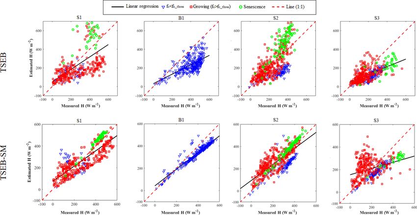
1782      B. Ait Hssaine et al.: An evapotranspiration model self-calibrated from remotely sensed surface soil moisture

quently allows the optimization of irrigation water applica-        uncertainties are observed during the quasi-senescent vege-
tions (Allen et al., 1998).                                         tation period (Boulet et al., 2015).
   Regarding the data availability over extended areas, re-            Alternatively to the use of LST as a proxy for ET, numer-
mote sensing is the only viable technique that can provide          ous studies have stressed that the soil moisture plays a criti-
representative and multi-resolution measurements of ET. As          cal role in the partitioning of available energy into latent and
a consequence, the spatial modeling has become a dominant           sensible heat fluxes and is the prominent controlling factor of
means of estimating ET fluxes over regional and continen-           actual ET (Boulet et al., 2015; Gokmen et al., 2012; Kustas
tal areas (Anderson et al., 2007; Fisher et al., 2017). In this     et al., 1998, 1999; Li et al., 2006). Several authors have re-
context, numerous models based on land surface tempera-             vised the well-known LST-based TSEB model and replaced
ture (LST) data have been developed, such as (i) residual           the LST with microwave-derived surface soil moisture (SM)
balance methods that consider ET to be the residual term            to estimate daily ET (Bindlish et al., 2001; Kustas et al.,
of the energy balance, like TSEB (two-source energy bal-            1998, 1999; Li et al., 2006). Bindlish et al. (2001) found
ance, Norman et al., 1995) and SEBS (surface energy balance         that the impact of SM on surface fluxes is strongly related
system, Su, 2002), (ii) contextual methods that estimate ET         to the vegetation cover. The impact is high for low fraction
as the potential ET times the evaporative efficiency (Moran         cover and relatively weak for the high cover fraction. More-
et al., 1994) or as the available energy times the evapora-         over, the soil evaporation is constrained by the SM through
tive fraction (Merlin et al., 2013; Roerink et al., 2000) and       its soil-texture-dependent coefficients (arss and brss ) reported
(iii) other categories of models that integrate LST into a wa-      in Sellers et al. (1992). In the same way, Li et al. (2006) in-
ter balance model (Olivera-Guerra et al., 2018) or into the         dicated that the model performance is sensitive to these two
Penman–Monteith energy balance (PMEB) equation to di-               coefficients, and thus they proposed averaging the output of
rectly estimate ET (Amazirh et al., 2017; Mallick et al., 2015,     LST-based TSEB and SM-based TSEB models in order to
2018).                                                              provide more consistent results over a wide range of condi-
   Among well-known temperature-driven energy flux mod-             tions.
els, the TSEB model proposed by Norman et al. (1995) has               Previous studies, either LST- or SM-based, agree with the
been shown to be robust for a wide range of landscapes (Co-         view that combining both LST and SM information at a
laizzi et al., 2012; Ait Hssaine et al., 2018a). TSEB has two       time would enhance the robustness and accuracy of ET es-
key input variables, which can be derived from remote sens-         timates in various biomes and climates. Nevertheless, few
ing data. The first one is the LST and the second is the vegeta-    studies have simultaneously combined both observations in
tion cover fraction (fc ). The TSEB model adopts an iterative       a unique energy balance model. One difficulty lies in devel-
procedure, in which an initial estimate of the plant transpira-     oping a consistent representation of the soil evaporation (as
tion is given by the Priestly–Taylor (PT) formulation (Priest-      constrained by SM, Chanzy and Bruckler, 1993), the total ET
ley and Taylor, 1972). This assumption requires few input           (as constrained by LST, Norman et al., 1995) and the plant
data and allows a precise estimate of potential ET (Fisher          transpiration (as indirectly constrained by both LST and SM,
et al., 2008). Nevertheless, several studies (Ait Hssaine et al.,   Ait Hssaine et al., 2018b).
2018b; Fisher et al., 2008; Jin et al., 2011; Yang et al., 2015)       Gokmen et al. (2012) explicitly integrated the SM derived
have stressed that the PT coefficient cannot be considered          from AMSR-E (Advanced Microwave Scanning Radiome-
a constant value, as it is influenced by several parameters.        ter for EOS) data (Owe et al., 2008) into the LST-derived
Other authors (Gonzalez-dugo et al., 2009; Long and Singh,          SEBS model via the kB −1 parameter, which plays an impor-
2012; Morillas et al., 2014) reported that the PT approach          tant role in the aerodynamic resistance. The updated SEBS
may overestimate the canopy ET, especially for low soil wet-        model (SEBS-SM) provided a large improvement of sensible
ness, and/or sparse vegetation cover, because it does not in-       heat flux and thus ET estimates under water-limited condi-
clude a reasonable reduction of the initial canopy ET under         tions. The point is that the soil evaporation reduction parame-
stress conditions. Recently, Boulet et al. (2015) developed         ters were calibrated using in situ measurements, which limits
the Soil-Plant-Atmosphere and Remote Sensing Evapotran-             the validity of the approach over large areas. In the same vein,
spiration (SPARSE) model, which is similar to the TSEB              Gan and Gao (2015) incorporated a SM-based soil resistance
model in its basic assumption but with additional constraints       term in the TSEB formalism and calibrated several parame-
to improve the ET model performance in heterogeneous veg-           ters (including the PT coefficient) using LST data. The ob-
etation. The former first generates an equilibrium LST from         tained results showed that the model calibrated by LST data
the evaporation efficiency and the transpiration efficiency es-     performed better than the non-calibrated one. Note that the
timates by assuming that their values are equal to 1. Then,         parameters of the soil resistance were set to constant values
LST is implemented in the SPARSE retrieval mode to cir-             as in Sellers et al. (1992) and Li et al. (2006). As a further
cumscribe the output fluxes by both limiting cases (namely          step towards the combination of LST and SM data, Ait Hs-
the fully stressed and potential conditions). In spite of the       saine et al. (2018b) modified the TSEB formalism (Kustas
good retrieval performances of ET by this model, significant        and Norman, 1999; Norman et al., 1995) (named TSEB-
                                                                    SM) and proposed a new calibration strategy of the main

Hydrol. Earth Syst. Sci., 24, 1781–1803, 2020                                     www.hydrol-earth-syst-sci.net/24/1781/2020/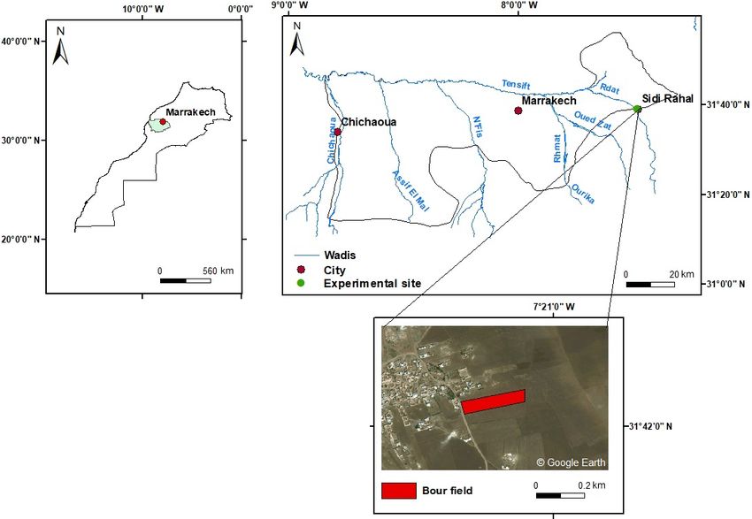
B. Ait Hssaine et al.: An evapotranspiration model self-calibrated from remotely sensed surface soil moisture                      1783

PT-based TSEB-SM parameters. The TSEB-SM model was                   Table 1. Characteristics of the study site.
tested using in situ measurements and provided an important
improvement in terms of latent heat flux/sensible heat flux               Study period                    Rainfall    Field status
estimates compared to the classic TSEB all along the agri-                                              amount (mm)
cultural season, especially during the crop emergence and                 Oct 2014–Jun 2015 (S1)             608      Cultivated
the senescence periods. Such improvements are attributed                  Aug 2015–Sep 2016 (B1)             157      Bare soil
to stronger constraints exerted on the representation of soil             Sep 2016–Jun 2017 (S2)             214      Cultivated
evaporation (via SM data and the calibrated soil parameters)              Oct 2017–Jun 2018 (S3)             481      Cultivated
and plant transpiration (via the calibrated daily PT coeffi-
cient). It should be noted that only LST and SM data are used
for the calibration of yearly arss and brss as well as daily αPT ,   evaporative demand around 1600 mm yr−1 according to the
while the flux measurements are needed only for the vali-            FAO method (Allen et al., 1998; Jarlan et al., 2015). Soil
dation of the TSEB-SM-simulated sensible and latent heat             is characterized by a fine texture with 47 % of clay, 33 %
fluxes.                                                              of loam and 18.5 % of sand (Er-Raki et al., 2007). The ex-
   One crucial point is that all the above studies based on          periment has been set up in a rainfed wheat (“Bour”) field
remotely sensed SM and LST have neglected the mismatch               since 2013 (Ali Eweys et al., 2017; Amazirh et al., 2018;
in the spatial resolutions of readily available SM products.         Merlin et al., 2018). Located within a larger area occupied by
Especially the global-scale SM data sets have a typical res-         rainfed wheat “Bour”, this field was chosen to be representa-
olution of 40–50 km (Entekhabi et al., 2010; Kerr et al.,            tive at a scale of 1 km, thus enabling the comparison between
2010; Njoku et al., 2003). Such spatial resolution is gener-         1 km resolution satellite-derived and localized in situ mea-
ally unsuitable or even incompatible with many hydrological          surements. The field was seeded in September 2014, Septem-
and agricultural applications. To fill the gap, disaggregation       ber 2016 and September 2017 for the 2014–2015 (S1), 2016–
approaches of AMSR-E, SMOS (Soil Moisture and Ocean                  2017 (S2) and 2017–2018 (S3) agricultural seasons, respec-
Salinity) and SMAP (Soil Moisture Active and Passive) like           tively. However, it was not ploughed (remained as bare soil)
SM data have been developed (Peng et al., 2017) but, to              during the 2015–2016 (B1) agricultural season due to an un-
date, there has been no application of SM-based ET models            usual lack of precipitation in autumn–winter 2015 (Merlin
to disaggregate SM data sets. In addition, the use of remote         et al., 2018) (Table 1).
sensing data would be necessary in order to avoid the time-             The field was instrumented by an eddy covariance (EC)
consuming process of calibrating the TSEB model over each            system at a 2 m height. EC tower includes a CSAT3 3-D sonic
field.                                                               anemometer that measures the wind and temperature fluctu-
   Although TSEB-SM has the capability to calibrate its              ations and a krypton hygrometer, KH20, that measures the
main parameters from remotely sensed data, the real-life ap-         concentration of water vapor. The EC tower is also equipped
plication needs extensive evaluation and testing. The objec-         with a CNR1 radiometer (Kipp and Zonen) to measure the
tive of this paper is thus to demonstrate for the first time this    four components of the net radiation (Rn ) with several heat
capacity using disaggregated SMOS and MODIS (MODer-                  flux plates (HFT3-L, Campbell Scientific Ltd) to measure the
ate resolution Imaging Spectroradiometer) data. For this pur-        soil heat flux (G). Energy balance closure analysis indicated
pose, TSEB-SM is applied to 1 km resolution using MODIS              that the available energy (Rn − G) was generally higher than
LST/fc data and to SMOS SM data. To make the SMOS                    the EC measurements. The relative closure was about 68 %,
data spatially consistent with MODIS data, the SMOS SM               76 %, 79 % and 79 % for S1, S2, S3 and B1, respectively.
is disaggregated at 1 km resolution using the DisPATCh               The sensible and latent heat fluxes (H and LE) were finally
(DISaggregation based on Physical And Theoretical scale              corrected to force the closure of the energy balance by the
Change) algorithm (Malbéteau et al., 2016; Merlin et al.,            Bowen ratio method (Twine et al., 2000). LST is measured
2013; Molero et al., 2016). The proposed methodology is              at the EC station by using two Apogee IRTS-P infrared ra-
evaluated over a rainfed wheat field in the Tensift basin, cen-      diometers, oriented downward and measuring the surface-
tral Morocco during four agricultural seasons (2014–2018).           leaving radiance between 8 and 14 µm, set up at a 2 m height
                                                                     above the ground. An estimate of LST is obtained by averag-
                                                                     ing both measurements. The soil water content is measured
2     Data description and methods                                   at various depths (5, 10, 20, 30, 50, 70 cm) using Time Do-
                                                                     main Reflectometry probes (model CS616) installed in a soil
2.1    Site and in situ data description                             pit at the bottom of the EC tower. A weather station was set
                                                                     up nearby the studied field to measure air temperature, so-
The study site is situated in the east (Sidi Rahal) of the Tensift   lar radiation, relative humidity, wind speed and rainfall at a
basin in central Morocco (see Fig. 1). The region is charac-         30 min time step.
terized by a semi-arid Mediterranean climate, with an aver-
age yearly precipitation of about 250 mm and an atmospheric

www.hydrol-earth-syst-sci.net/24/1781/2020/                                        Hydrol. Earth Syst. Sci., 24, 1781–1803, 2020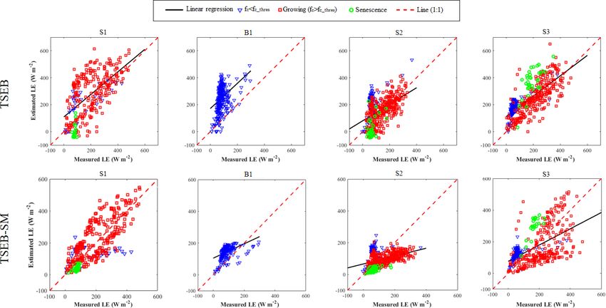
1784         B. Ait Hssaine et al.: An evapotranspiration model self-calibrated from remotely sensed surface soil moisture

Figure 1. Location of the Sidi Rahal site (east of Marrakech) in the Tensift basin, central Morocco.

2.2     Remote sensing data
                                                                         fc = 1 − exp(−0.5LAI).                                     (2)
2.2.1    MODIS
                                                                         Finally, the MCD43A3 product provides the surface
Three products from the MODIS sensor onboard the                         albedo (α) at 500 m resolution every 16 d. The latter is gener-
Terra and Aqua satellites are used in this study: the                    ated from both the Terra and Aqua products. In this work, the
(1) MODIS Terra/Aqua Land Surface Temperature product                    shortwave broadband α is used by integrating its value over
(MOD11A1/MYD11A1), the (2) MODIS Terra Vegetation                        the entire solar emission spectrum (0.3–5.0 µm). This value
Indices product (MOD13A2) and the (3) MODIS Albedo                       is obtained as a weighted average of the directional hemi-
(combined Terra and Aqua) product (MCD43A3). All prod-                   spherical reflectance (black-sky-α) and the bi-hemispherical
ucts are gridded in the sinusoidal projection.                           reflectance (white sky α) using their two extreme values. The
   The MOD11A1 and MYD11A1 provide LST at 1 km                           current α (called “blue sky”) is a weighted average between
spatial resolution under clear-sky conditions, derived from              these two extreme cases (Lewis and Barnsley, 1994). Herein,
Terra and Aqua, respectively. Brightness temperatures from               the percentages of 85 % and 15 % are used for the direct and
bands 31 and 32 are used to derive LST through a general-                diffuse lights, respectively.
ized split-window algorithm. The MOD13A2 provides sev-
eral vegetation indices at 1 km resolution. One particular veg-          2.2.2   SMOS
etation index of interest in this study is NDVI, available at 16-
day temporal intervals. This product is derived from bands 1             The SMOS mission measures the natural (passive) mi-
and 2 of the MODIS Terra satellite.                                      crowave radiation around the frequency of 1.4 GHz (L-band).
   The obtained NDVI is used to derive the leaf area in-                 It aims to monitor SM at a depth of about 3–5 cm with
dex (LAI) via the following formulation (Wang et al., 2013):             a spatial resolution of about 40 km and an accuracy better
                                                                         than 0.04 m3 m−3 (Kerr et al., 2012). The revisiting time

             1 + NDVI
                                1/2                                     at the Equator is 3 d for both ascending and descending
LAI = NDVI ×                           .                        (1)      passes, which are Sun synchronous at 06:00 and 18:00 LT,
             1 − NDVI
                                                                         respectively. The SMOS level-3 1 d global SM product
The vegetation cover fraction is expressed as (Kustas and                (MIR CLF31A/D) posted on the ∼ 25 km Equal Area Scal-
Norman, 1997)                                                            able Earth (EASE) version 1.0 grid is used as input to the
                                                                         DisPATCh algorithm.

Hydrol. Earth Syst. Sci., 24, 1781–1803, 2020                                           www.hydrol-earth-syst-sci.net/24/1781/2020/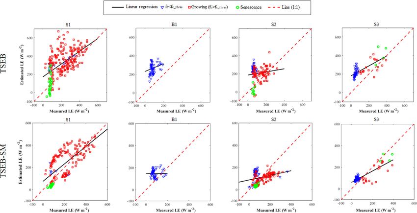
B. Ait Hssaine et al.: An evapotranspiration model self-calibrated from remotely sensed surface soil moisture                       1785

2.2.3    DisPATCh                                                        The vegetation latent heat flux LEveg is estimated via the
                                                                       PT formulation:
The DisPATCh remote sensing algorithm combines the
coarse-scale microwave-retrieved SM with high-resolution                                     4
                                                                       LEveg = αPT · fg ·       · Rn,veg ,                            (4)
optical/thermal data within a downscaling relationship to                                   4+γ
produce SM at a higher spatial resolution.
                                                                       where αPT is the PT coefficient, fg the fraction of green veg-
   Soil (Ts,min , Ts,max ) and vegetation (Tv,min , Tv,max ) temper-
                                                                       etation, γ the psychometric constant (≈ 67 Pa K−1 ), 4 the
ature endmembers are estimated from the polygon obtained
                                                                       slope of the relationship between saturation vapor pressure
by plotting MODIS LST against MODIS NDVI, where the
                                                                       and air temperature, and Rn,veg the vegetation net radia-
LST is partitioned into its soil and vegetation components
                                                                       tion. Note that fg is set to 1 as the αPT coefficient is varied
according to the trapezoid method of Moran (Moran et al.,
                                                                       (through the calibration procedure) to take into account the
1994). Details on the DisPATCh algorithm and the method-
                                                                       fraction of transpiring vegetation. The soil latent heat flux is
ology to determine dry and wet edges can be found in Mer-
                                                                       estimated using the resistance formulation:
lin et al. (2012). The retrieved soil temperature is then used
to estimate the soil evaporative efficiency (SEE), which is                       ρcp es − ea
defined as the ratio of actual to potential soil evaporation.          LEsoil =                     ,                                 (5)
                                                                                   γ rah + rs + rss
Finally, DisPATCh converts the high-resolution optically de-
rived SEE fields into high-resolution SM fields given a semi-          where es is the saturated vapor pressure at the soil surface,
empirical SEE model and a first-order Taylor series expan-             ea the actual air vapor pressure, rah the aerodynamic resis-
sion around the SMOS observation. In our application, we               tance calculated from the adiabatically corrected logarith-
applied DisPATCh to 40 km resolution SMOS level-3 SM                   mic temperature profile equation (Brutsaert, 1982) and rs the
and 1 km resolution MODIS optical/thermal data to pro-                 surface-soil resistance to transport of heat between the soil
duce SM at a 1 km resolution (Molero et al., 2016). The input          surface and a height representing the canopy estimated us-
data sets are composed of MODIS LST, MODIS NDVI and                    ing (Sauer et al., 1995). Both resistances are simulated every
the GTOPO digital elevation model (DEM) used to correct                30 min (between 11:00 and 14:00 LT) and at Terra and Aqua
LST for topographic effects (Malbéteau et al., 2016; Merlin            overpass times for in situ and satellite data, respectively. rss is
et al., 2013).                                                         computed as a function of SM and is expressed as (Chirouze
                                                                       et al., 2014; Li et al., 2006; Sellers et al., 1992)
2.3     Methods
                                                                                                   SM
                                                                       rss = exp arss − brss ×            ,                           (6)
2.3.1    TSEB-SM                                                                                  SMsat

The recently developed TSEB-SM is fully described in                   with SM being the 0–5 cm SM, arss and brss are two empirical
Ait Hssaine et al. (2018b). The equations and sub-equations            parameters (to be calibrated) and SMsat is the SM at satura-
used in TSEB-SM are provided in Table 2; the main equa-                tion expressed as (Cosby et al., 1984)
tions are given below. The originality of TSEB-SM is to in-
tegrate SM observations in addition to LST and vegetation              SMsat = 0.1 × (−108 × fsand + 49.305) ,                        (7)
cover fraction data in order to calibrate both the soil resis-
tance to evaporation (constant parameters) and the PT coef-            with fsand being the sand percentage of soil.
ficient on a daily basis. The model is based on the original             In Ait Hssaine et al. (2018b), an innovative calibration ap-
TSEB formalism, meaning that the energy balance for vege-              proach of αPT , arss and brss is developed from in situ SM and
tation is the same as in TSEB using the PT formula, although           LST data (Ait Hssaine et al., 2018b). The calibration method-
the soil evaporation is estimated as a function of SM using a          ology is briefly explained below.
soil resistance developed by Sellers et al. (1992). The use of
                                                                       Retrieval and calibration of rss , arss and brss
the soil resistance formulation is justified by the fact that its
main parameters (arss , brss ) can be adjusted based on soil tex-      The rss is first adjusted by minimizing a cost function defined
ture characteristics (Merlin et al., 2016) or by combining SM          by
and LST data under bare (Merlin et al., 2018) or partially
covered (Ait Hssaine et al., 2018b) soil conditions.                                                2
                                                                       Finst = Tsurf,sim − Tsurf,mes ,                                (8)
   The surface soil heat flux is estimated as a fraction
of Rn,soil :                                                           with Tsurf,sim and Tsurf,mes being the simulated and measured
                                                                       LST, respectively.
G = cg · Rn,soil ,                                              (3)
                                                                         The Tsurf,sim was simulated as follows:
where cg ∼ 0.35 (Choudhury et al., 1987).                                                  4                       0.25
                                                                       Tsurf,sim = fc · Tveg + (1 − fc ) · (Tsoil )4       ,          (9)

www.hydrol-earth-syst-sci.net/24/1781/2020/                                          Hydrol. Earth Syst. Sci., 24, 1781–1803, 2020
1786 B. Ait Hssaine et al.: An evapotranspiration model self-calibrated from remotely sensed surface soil moisture
Table 2. Mean equations of TSEB-SM.
Variable Equation Value range
ρc
Soil latent heat flux LEsoil = γ p rahe+r
s −ea
s +rss
0–600 W m−2
Resistance to vapor diffusion in the soil SM
rss = exp arss − brss × SM arss and brss : (1–13)
sat
Soil moisture at saturation SMsat = 0.1 × (−108 × fsand + 49.305) 0.47 m3 m−3
2
Cost function for minimizing rss Fins = Tsurf,sim − Tsurf,mes Finst = 5 K
Vegetation latent heat flux 1 R
LEveg = αPT Fg 1+γ αPT (0–2) fg = 1
n,veg
where Tveg and Tsoil are the vegetation and soil components Elguero, 1999; Shuttleworth et al., 1989) and the EF has
of temperature (K). The LST is simulated every 30 min (be- a strong link with SM availability (Bastiaanssen and Ali,
tween 11:00 and 14:00 LT) and at Terra and Aqua overpass 2003), which is an important factor for estimating latent
times for in situ and satellite data, respectively. The LST at heat flux. For that purpose, the LST data collected at the
the first calibration step is simulated with a constant value Terra and Aqua-MODIS overpass times are used to estimate
of αPT (average value of the αPT retrieved for fc > 0.5). the instantaneous Rn and G. A ratio between the daily (ob-
Then, for the second calibration step, it is simulated using tained as an average value between Aqua and Terra overpass
the daily retrieved αPT . times) latent heat flux LEdaily and the daily available energy
The inverted rss is then correlated with the SM (in situ (Rn,daily − Gdaily ) is used to calculate an average daily EF:
or DisPATCh) to determine the arss and brss parameters by
considering that, when fc is lower than a given thresh- LEdaily
EF = . (11)
old (fc,thres ), the dynamics of total LE is mainly controlled Rn,daily − Gdaily
by the temporal variation of soil evaporation, meaning that
both soil parameters are estimated when the PT coefficient The daily EF and the instantaneous available energy (calcu-
can be set to a constant value. lated using Terra and Aqua MODIS LST) are finally used
to re-calculate the instantaneous TSEB-SM output of LE
Daily αPT retrieval and H by the following formulas:
Once both parameters arss and brss have been estimated, the LE = EF × (Rn − G) , (12)
PT coefficient is retrieved on a daily basis when fc is larger H = (1 − EF) × (Rn − G) . (13)
than fc,thres , by minimizing a cost function at the Terra and
Aqua-MODIS overpass times: 2.3.2 Uncertainty in TSEB-SM input data
X 2
Fdaily = Tsurf,sim − Tsurf,mes . (10) The LST collected by MODIS at Terra and Aqua overpass
times and the SM product derived at 1 km resolution from
In fact, an iterative loop is run on soil (rss ) and vegeta- the DisPATCh algorithm applied to SMOS data are used as
tion (αPT ) parameters to reach convergence of all parameters. input to TSEB and TSEB-SM models. Validation of TSEB
LST and SM data are thus used for calibration, while the cal- and TSEB-SM input data prior to the evaluation of model
ibrated TSEB-SM is run on a daily basis using SM data as output is an important issue, because of the scale discrepancy
forcing solely (in addition to vegetation cover fraction data). between the spatial resolution (1 km) of MODIS/DisPATCh
In this paper, an improvement is made on the former ver- data and the footprint of the EC flux measurements that does
sion of TSEB-SM to normalize the output fluxes using the not exceed 100 m (Schmid, 1994).
LST-derived available energy. Therefore, the new version of Several studies have demonstrated the effectiveness of
TSEB-SM uses both LST and SM data (in addition to veg- DisPATCh 1 km resolution SM. Malbéteau et al. (2016) com-
etation cover fraction data) as forcing on a daily basis. In pared DisPATCh SM data with the in situ measurements col-
practice, the latent and sensible heat fluxes derived from the lected in the Murrumbidgee catchment in southeastern Aus-
TSEB-SM model are re-computed using the TSEB-SM de- tralia. Their results showed that DisPATCh improved the spa-
rived evaporative fraction (EF, defined as the ratio of latent tial representation of SM at 1 km resolution (compared to the
heat to available energy) and the LST-derived available en- original 40 km resolution SMOS SM), especially in semi-
ergy. The rationale is that numerous modeling studies have arid areas. Recently, Malbéteau et al. (2018) combined the
shown the regularity and constancy of EF during daylight DisPATCh SM over the entire year 2014 (Sidi Rahal, Mo-
hours in cloud-free days (Gentine et al., 2011; Lhomme and rocco) with the continuous predictions of a surface model in
Hydrol. Earth Syst. Sci., 24, 1781–1803, 2020 www.hydrol-earth-syst-sci.net/24/1781/2020/B. Ait Hssaine et al.: An evapotranspiration model self-calibrated from remotely sensed surface soil moisture 1787
Figure 2. Scatterplots of MODIS versus in situ LST at the Sidi Rahal site for the S1 (2014–2015), B1 (2015–2016), S2 (2016–2017) and
S3 (2017–2018) agricultural seasons, separately, (red dashed line is the 1 : 1 line; black line is the regression line).
order to obtain a better estimate of daily SM at 1 km reso- Table 3. Validation results of DisPATCh SM and MODIS LST at
lution. They found that the assimilation of DisPATCh data the Sidi Rahal site.
improved quasi-systematically the dynamics of SM.
Figure 2 shows the scatterplots of MODIS LST (at Terra Period R2 RMSE MBE
and Aqua overpass) versus in situ measurements for the four S1 0.8 6.4 (K) −3.7 (K)
agricultural seasons separately. The obtained R 2 , root mean B1 0.76 5.6 (K) −4.6 (K)
LST
square error (RMSE), and mean bias error (MBE) are re- S2 0.91 4.3 (K) −2.9 (K)
ported in Table 3. The statistical comparison shows strong S3 0.89 4 (K) −2 (K)
linear correlations (0.76 ≤ R 2 ≤ 0.90) for all years. The
S1 0.55 0.07 m3 m−3 −0.04 m3 m−3
RMSE is around 4 K for the S2 (2016–2017) and S3 (2017–
B1 0.36 0.04 m3 m−3 −0.03 m3 m−3
2018) agricultural seasons, while it reaches 6 K for S1 (2014– SM
S2 0.27 0.09 m3 m−3 −0.05 m3 m−3
2015) and B1 (2015–2016), respectively. The observed scat- S3 0.47 0.08 m3 m−3 −0.03 m3 m−3
ter may stem from the fact that the localized (1 or 2 m wide)
in situ LST is not fully representative of the 1 km resolution
MODIS pixel (Ait Hssaine et al., 2018a; Yu et al., 2017). For
all years (S1–3, B1), it can be seen that the MBE is negative. (Bandara et al., 2015; Colliander et al., 2017; Djamai et al.,
Note that the MBE is the greatest when the temperatures are 2015; Escorihuela and Quintana-Seguí, 2016; Escorihuela
largest. Such a systematic error is probably due to the non- et al., 2018; Lievens et al., 2015; Malbéteau et al., 2016,
representativeness of the in situ LST observations when com- 2018; Merlin et al., 2012; Merlin et al., 2013; Merlin et al.,
pared to the corresponding scale of MODIS observations. 2015; Molero et al., 2016; Ojha et al., 2019; Peng et al., 2017;
The DisPATCh products have been extensively evaluated, Sabaghy et al., 2020). Actually, the scatterplots of Fig. 3
especially over semi-arid areas like the Marrakech region aim to verify that the DisPATCh soil moisture is consistent,
www.hydrol-earth-syst-sci.net/24/1781/2020/ Hydrol. Earth Syst. Sci., 24, 1781–1803, 20201788 B. Ait Hssaine et al.: An evapotranspiration model self-calibrated from remotely sensed surface soil moisture
Figure 3. Scatterplots of the 1 km resolution DisPATCh versus in situ SM at the Sidi Rahal site for the S1 (2014–2015), B1 (2015–2016),
S2 (2016–2017) and S3 (2017–2018) agricultural seasons, separately.
during four agricultural seasons (S1, B1, S2 and S3), at the ing on soil conditions (notably SM content, texture). For S2,
site level where the comparison between TSEB and TSEB- the SM provided by DisPATCh underestimated field mea-
SM is undertaken. The statistical results including the co- surements, especially in the higher SM range. This particular
efficient of determination (R 2 ), the RMSE, and the MBE behavior could be explained by the particularly low precip-
are reported in Table 3. The R 2 ranges from 0.27 to 0.55, itation amount during this year. It is especially possible that
the RMSE from 0.04 to 0.09 m3 m−3 and the MBE from the surrounding plots were not sown by neighboring farmers,
−0.05 to −0.03 m3 m−3 . These results are encouraging con- resulting in a soil that dried quickly compared to our field,
sidering the heterogeneous land use composed of rainfed which retained the SM for a longer period of time.
wheat, bare soil, and fallow and farm building (see Fig. 4). Note that despite the relative heterogeneity within the 1 km
In fact, the localized in situ measurements may not be per- pixel (characterized by rainfed wheat in addition to bare soil
fectly representative of the 1 km resolution satellite data. and fallow), the comparison between field measurements and
Note that the efficiency of DisPATCh is supposedly higher 1 km resolution satellite data reflects acceptable accuracies.
for low SM values (Malbéteau et al., 2016), which is clearly
illustrated during the B1 season, while it is lower for high
SM values (after rain events). This can be explained by the 3 Results and discussion
constraints of atmospheric and vegetation conditions on dis-
In this section, the arss and brss parameters and the αPT are
aggregation results as well as the saturation of SEE in the
firstly retrieved by following the two-step calibration based
higher SM range. Another major issue that can lead to differ-
on a threshold of fc (cited in the Methods section). Then,
ences between DisPATCh and in situ SM is that the ground
the obtained calibrated values are used to estimate the sur-
SM sensors are buried at a depth of 5 cm, while the penetra-
face fluxes using TSEB-SM. Finally, TSEB-SM fluxes are
tion of the L-band wave varies between 2 and 5 cm depend-
evaluated against the eddy covariance measurements, and re-
Hydrol. Earth Syst. Sci., 24, 1781–1803, 2020 www.hydrol-earth-syst-sci.net/24/1781/2020/B. Ait Hssaine et al.: An evapotranspiration model self-calibrated from remotely sensed surface soil moisture 1789
Figure 4. NDVI image derived from Landsat data acquired on 17 April 2018. The experimental field and the overlaying 1 km resolution
MODIS pixel are superimposed.
sults are compared with the original TSEB. To facilitate the empirical nature of the rss . Another major issue that can lead
interpretation of the simulation results using MODIS and to these differences is the depth of SM measurements (Mer-
SMOS/DisPATCh data as input, the calibration and valida- lin et al., 2011). In Sellers et al. (1992), the near-surface soil
tion steps are previously tested using in situ (LST and SM) moisture is defined in the 0–5 cm soil layer, whereas in our
data. field, SM measurements are made at 5 cm depth. Also, the
sensing depth of SMOS observations is generally shallower
3.1 Retrieving arss and brss parameters than the in situ surface measurements (Escorihuela et al.,
2010). Moreover, the variability of arss and brss in Fig. 5b
The soil resistance rss is inverted for fc ≤ fc,thres between using remote sensing data can be linked to the scale differ-
11:00 and 14:00 LT and at the Terra and Aqua overpass time ence between DisPATCh SM/MODIS products (1 km) and
step for in situ and satellite data, respectively. The result of the field measurements. As shown in Fig. 3, the field is sur-
this inversion is correlated with the actual to saturated soil rounded by trees, buildings and fallows, which causes the
moisture ratio SM/SMsat to determine arss and brss parame- spatial heterogeneity within the pixel of 1 km. This hetero-
ters. The calibration process is applied for each season inde- geneity can introduce errors into the model inversion. Never-
pendently. Then a pair (arss , brss ) is calculated for the entire theless, soil parameters are quite similar for in situ and satel-
study period for in situ and satellite data, respectively. lite data sets. Therefore, the heterogeneity issues within the
Figure 5a and b plot the ln(rss ) versus in situ SM/SMsat 1 km pixel scale are minor in this study.
using in situ and satellite data, respectively. The mean re-
3.2 Time series of daily retrieved αPT
trieved values (7.62, 2.43) and (7.32, 4.58) for in situ and
satellite data, respectively, are close to the values found in The second calibration step consists in inverting the daily αPT
Li et al. (2006) (8.2, 4.3) and in Ait Hssaine et al. (2018b) when vegetation is covering a significant part of soil (fc >
(7.2, 4). However, by comparing both figures (Fig. 5a and b), fc,thres ), for the three seasons of rainfed wheat (S1–S3), by
one notes that the use of in situ data generates more scatter using in situ data and satellite data, separately. Herein, the
than with satellite data. The apparent scatter in retrieved rss calibration of αPT is bounded by minimum (0) and maxi-
could be interpreted by the impact of the daily cycle of mete- mum (2) acceptable physical values, in order to avoid un-
orological (evaporative demand) conditions or soil property acceptable values of αPT that can be produced because of the
differences (Merlin et al., 2011; Merlin et al., 2016; Merlin uncertainties in daily LST estimates. Such an upper bound-
et al., 2018). The retrieved soil parameters also vary from ing is especially needed when vegetation partially covers the
year to year: the standard deviation is 0.39 and 1.69 for arss soil.
and brss , respectively. This can be explained by the compen-
sation effects linking arss and brss parameters which prove the
www.hydrol-earth-syst-sci.net/24/1781/2020/ Hydrol. Earth Syst. Sci., 24, 1781–1803, 20201790 B. Ait Hssaine et al.: An evapotranspiration model self-calibrated from remotely sensed surface soil moisture
Figure 5. ln(rss ) versus SM/SMsat (calibration step 1) using in situ (a) and satellite (b) data.
3.2.1 Using in situ data that the stability of αPT strongly depends on the rainfall dis-
tribution along the agricultural season. The daily αPT is more
Figure 6 plots the daily variation of αPT for each season (S1– stable for S1 than for S2 and S3. Indeed, the amount of rain
S3) separately, using in situ data. The mean retrieved values during S1 is very important, with two peaks of about 83 mm
of αPT are 1.26, 1.12 and 1.09 for S1, S2 and S3, respec- that occurred at the beginning of the season and during the
tively. In all cases, the mean αPT is close to the theoretical growing stage. The second one coincides exactly with the
αPT value (1.26). It is well observed that the retrieved αPT maximum value of the retrieved αPT . However, different re-
for S1 is slightly larger compared to those obtained for sults are obtained for S2 compared to S1 due to the lowest
both S2 and S3. This can be explained by the timing and precipitation amount recorded over that season. As shown in
amount of rainfall during each season. Note that unexpected Fig. 6, the amount of rain is concentrated at the beginning
low values of αPT are recorded for S3 during the first few of the growing stage (mid December), when the αPT peaks.
days (25 January–4 March) of the development stage. They Afterward, the smoothed αPT tends to decrease because of in-
may be associated with uncertainties in retrieved αPT , as the sufficient soil water reserve in the root zone to enable wheat
impact of soil surface is still significant, as well as with a to continue growing. Rainfall is also significant for S3, and
relatively low evaporative demand especially since this pe- every rainfall event causes an immediate (daily) response
riod coincides with cloudy days and abundant precipitations. of αPT (after 4 March). As mentioned before, the signifi-
Indeed, the coupling between transpiration (and hence re- cant error in αPT retrievals for S3 between 25 January and
trieved αPT ) and LST is expected to be lower under lower 4 March induces strong uncertainties in the smoothing func-
atmospheric demand. tion estimates.
The retrieved αPT is then smoothed as in Ait Hssaine et al.
(2018b) to remove outliers and to reduce uncertainties at the 3.2.2 Using satellite data
daily timescale. The smoothed values of αPT range from 0
to 1.54, 0 to 1.38 and 0.45 to 1.43 for S1, S2 and S3, respec- Figure 6 also illustrates the daily variation of αPT retrieved
tively. The maximum of αPT is close to 1.26 for S2, while it is from satellite data for each season separately. S1 and S2 have
higher for S1 and S3. This result is in accordance with the to- a very similar distribution of the retrieved αPT as compared
tal rainfall amounts, which were about 608, 214 and 421 mm to the retrieved αPT using in situ data, respectively. For S3,
for S1, S2 and S3, respectively. Additionally, one can state only six retrieved αPT values are available because of the
Hydrol. Earth Syst. Sci., 24, 1781–1803, 2020 www.hydrol-earth-syst-sci.net/24/1781/2020/B. Ait Hssaine et al.: An evapotranspiration model self-calibrated from remotely sensed surface soil moisture 1791
Figure 6. Time series of daily retrieved and smoothed αPT (calibration step 2 – using in situ data and satellite data) collected during S1, S2
and S3.
non-availability of MODIS products during cloudy days. For maximum value of NDVI appears sooner than the maximum
this reason, no information linked to the variability of αPT value of αPT for both S1 and S3. Such a delay is attributed to
can be derived during this season. The retrieved values are the high soil moisture level in the root zone during the matu-
smoothed and superimposed with the rainfall events. It is rity stage. Later in the season, αPT decreases as NDVI starts
clearly shown that the smoothed αPT for S1 and S2 have the to decline at the onset of senescence. In contrast, the maxi-
same shape with a small variability when compared with the mum value of NDVI appears later than the maximum value
smoothed αPT using in situ data, resulting in an error esti- of αPT for S2. This can be explained by the fact that rainfall
mated as the RMSE to the mean αPT ratio, of about 11 % and at the beginning of the development phase satisfies the plant
19 %, for S1 and S2, respectively. For S1 the maximum of requirements, while the rainfall amount during the develop-
smoothed αPT is reached at the same time as when using the ment stage is relatively low compared to the crop water needs
in situ data, with a value of about 1.38, while the maximum (Kharrou et al., 2011). Large variations in αPT occur during
for S2 is reached 10 d before the maximum of the αPT derived the agricultural season, as a result of the amount, frequency,
from in situ data with little response of αPT to rainfall events. and distribution of rainfall along the season. In general, the
These differences may be linked to uncertainties in disag- analysis of the αPT variability using satellite data illustrates
gregated SMOS SM as well as to the weaker availability of the robustness of the proposed approach, which combines
satellite data. Because of the small number of data points (re- microwave and optical/thermal data to retrieve a water stress
trieved αPT ) during S3, the smoothed αPT remains at a mostly indicator at the daily timescale.
constant value (∼ 0.7) throughout the study period, with a
significant relative difference of about 34 % when compared 3.3 Surface fluxes
with the αPT retrieved using in situ data.
The robustness of TSEB and TSEB-SM for partitioning
3.2.3 Interpretation of αPT variabilities (Rn − G) into H and LE is evaluated using in situ and re-
motely sensed LST, SM, and NDVI, separately, at Terra and
Figure 7 plots variation of calibrated daily αPT , superim- Aqua MODIS overpasses.
posed with NDVI and rainfall events. It is visible that the
www.hydrol-earth-syst-sci.net/24/1781/2020/ Hydrol. Earth Syst. Sci., 24, 1781–1803, 20201792 B. Ait Hssaine et al.: An evapotranspiration model self-calibrated from remotely sensed surface soil moisture
Figure 7. Time series of calibrated daily αPT (red – using in situ data, green – using satellite data) superimposed with NDVI and the rainfall
events during S1, S2 and S3, separately.
3.3.1 Using in situ data high for a bare soil, which yields a slight overestimate of
LE measurements (see the B1 case in Fig. 8).
For the S3 season, the error in daily retrieved αPT at the
Figure 8 shows an intercomparison of simulated and ob- beginning of the development stage has a strong impact on
served LE for the four seasons separately. TSEB-SM clearly LE predictions and thus yields to greater discrepancies illus-
provides improved results compared to the original TSEB. trated in Fig. 8. To overcome this error, the threshold on fc to
The obtained values of RMSE by TSEB-SM are about 68 and separate calibration steps 1 and 2 was increased to 0.63 (arbi-
72 W m−2 for S1 and S2, respectively, which is significantly trary value). The TSEB-SM model is then run using the new
lower than those revealed by TSEB (109 and 86 W m−2 , re- threshold. The LE simulations are improved, with a RMSE
spectively) (see Table 4). For B1 (season of bare soil), TSEB of 73 W m−2 instead of 98 W m−2 and a relative error (es-
largely overestimates LE with a MBE of about 165 W m−2 timated as the RMSE divided by the mean observed LE)
compared to TSEB-SM, which yields a MBE of 59 W m−2 . of about 42 % instead of 58 %. The increase in the thresh-
This overestimation of TSEB is most probably related to an old is intended to decrease the uncertainties in αPT retrievals
inadequate value of αPT (= 1.26) for bare soil surfaces. In when vegetation is not fully covering the soil. It can be con-
fact, 1.26 is an optimum value for the potential transpiration cluded that the errors in αPT retrievals have a strong impact
rate (Agam et al., 2010; Chirouze et al., 2014). In the case on LE estimates.
of TSEB-SM, biases are reduced thanks to the calibration of The ability of TSEB-SM to estimate the sensible heat
the rss resistance. Additionally, according to TSEB-SM as- fluxes is also investigated. Figure 9 displays the compari-
sumptions, αPT for fc ≤ 0.5 is set to the average value of the son between TSEB and TSEB-SM for each season and Ta-
αPT retrieved for fc > 0.5. During the B1 season (bare soil ble 4 summarizes the different statistical parameters. One
conditions), αPT was hence obtained as an average value of can notice that TSEB shows greater discrepancies in H es-
the mean αPT retrieved for all seasons S1, S2 and S3 when timation, with a RMSE of about 127, 112 and 103 W m−2
fc > 0.5 (αPT ∼ 1). However, this value remains relatively and a MBE of about −41, 1, and −71 W m−2 for S1, S2 and
Hydrol. Earth Syst. Sci., 24, 1781–1803, 2020 www.hydrol-earth-syst-sci.net/24/1781/2020/B. Ait Hssaine et al.: An evapotranspiration model self-calibrated from remotely sensed surface soil moisture 1793
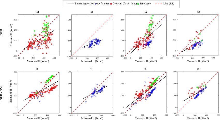
Figure 8. Scatterplot of simulated versus observed LE for (top panels) TSEB and (bottom panels) TSEB-SM models using in situ data
collected during S1, B1, S2 and S3, respectively.
Table 4. Statistical results (RMSE, R 2 and MBE) between modeled and measured sensible and latent heat fluxes for S1, S2, B1 and S3, and
for TSEB and TSEB-SM models, separately (Rn and G are forced to their measured value). Bold values are the values with better statistical
results.
TSEB TSEB-SM
RMSE R2 MBE RMSE R2 MBE
S1 109 0.39 76 68 0.59 10
B1 136 0.15 165 52 0.22 59
LE (W m−2 )
S2 86 0.22 30 72 0.16 −24
S3 103 0.53 71 98 0.29 –7
Using in situ data
S1 127 0.33 −41 68 0.7 –10
B1 136 0.44 −165 52 0.91 –59
H (W m−2 )
S2 112 0.47 1 72 0.63 24
S3 103 0.38 −71 98 0.14 7
S1 95 0.34 119 55 0.51 39
B1 66 0.07 181 27 0.01 62
LE (W m−2 )
S2 67 0.02 94 41 0.08 4
S3 56 0.55 128 24 0.68 7
Using satellite data
S1 98 0.3 −104 55 0.54 –39
B1 66 0.37 −181 27 0.52 –62
H (W m−2 )
S2 73 0.33 −71 41 0.6 –4
S3 56 0.28 −128 24 0.36 –7
www.hydrol-earth-syst-sci.net/24/1781/2020/ Hydrol. Earth Syst. Sci., 24, 1781–1803, 20201794 B. Ait Hssaine et al.: An evapotranspiration model self-calibrated from remotely sensed surface soil moisture
Figure 9. Same as Fig. 8 but for H fluxes.
S3, respectively. Both RMSE and MBE values are generally estimates. Indeed, as reported in Table 5, Rn is very well
much reduced when using TSEB-SM, with RMSE values of simulated for both TSEB and TSEB-SM. The R 2 between
about 68, 72, and 98 W m−2 and MBE values of about −10, simulated and observed Rn is about 0.99 during all seasons.
24, and 7 W m−2 , respectively. During B1, TSEB model un- Meanwhile, G shows a poor correlation, with an R 2 varying
derestimates H . This can be explained by the low sensi- from 0.05 to 0.45. This is mainly linked to the approach used
tivity of simulated sensible heat flux to changes in surface to estimate G, which requires local calibration. Kustas et al.
and atmospheric conditions, consistent with former results (1998) hence indicated that the ratio G/Rn,soil cannot be con-
obtained on different sites of irrigated wheat (Ait Hssaine sidered a constant, because it is affected by different factors
et al., 2018b). The discrepancies between TSEB-SM and in such as time of day, moisture conditions and soil texture and
situ H during S3 are mostly rectified by using the new thresh- structure.
old on fc : the statistical results are improved, the RMSE
is about 73 W m−2 and the relative error is 39 % (instead 3.3.2 Using satellite data
of 52 %). It can be concluded that the uncertainty observed
over the αPT during the first few days of the development In order to gain greater insight into how TSEB and TSEB-
stage (25 January–4 March) is mainly related to the impact SM models respond to different surface conditions across
of the soil, which is not negligible during the first weeks of a landscape, an analysis of the spatial distributions and the
the growing stage. Nevertheless, by considering the over- magnitude of the turbulent fluxes using remotely sensing data
all results obtained for the three seasons, the threshold of produced from the two models is conducted. The compar-
fc,thres = 0.5 can be considered an acceptable value to cal- isons between TSEB/TSEB-SM versus observed LE over
ibrate the soil resistance parameters and the Priestly–Taylor the four seasons are illustrated in Fig. 10. Figure 10 indi-
coefficient. cates that TSEB overestimates latent heat flux. The overall
As a further step, the intercomparison between TSEB and MBE values are about 119, 181, 94 and 128 W m−2 for S1,
TSEB-SM is evaluated by predicting Rn and G fluxes instead B1, S2 and S3, respectively. The overestimation of LE fluxes
of forcing them to their measured values. The statistical re- can be explained by the fact that αPT is set to 1.26 dur-
sults of the comparison between simulated and observed Rn , ing the entire agricultural season including stress conditions.
G, H and LE are listed in Table 5. The scattering obtained This probably causes larger errors in the LE estimation, es-
when comparing turbulent flux estimations to measurements pecially during the growing stage. Indeed, the saturation of
is mainly related to the uncertainty in available energy es- TSEB during the senescence period is precisely caused by
timates, mainly related to the uncertainty in soil heat flux the PT coefficient fixed to 1.26. The errors are reduced when
using TSEB-SM. In fact, the constraint on plant transpira-
Hydrol. Earth Syst. Sci., 24, 1781–1803, 2020 www.hydrol-earth-syst-sci.net/24/1781/2020/B. Ait Hssaine et al.: An evapotranspiration model self-calibrated from remotely sensed surface soil moisture 1795 Figure 10. Same as Fig. 8 but for satellite data. Figure 11. Same as Fig. 8 but for H fluxes and satellite data. www.hydrol-earth-syst-sci.net/24/1781/2020/ Hydrol. Earth Syst. Sci., 24, 1781–1803, 2020
1796      B. Ait Hssaine et al.: An evapotranspiration model self-calibrated from remotely sensed surface soil moisture

Figure 12. αPT vs. residual H and LE error.

tion, while retrieving daily αPT values improves ET esti-          outputs. The RMSE is significantly improved from 103 to
mates, especially for the growing stage. Moreover, during the      52 W m−2 , from 151 to 30 W m2 , from 101 to 35 W m−2 and
senescence stage the large positive bias of LE is consider-        from 83 to 24 W m−2 , during S1, B1, S2 and S3, respectively.
ably reduced. In fact, the decrease in calibrated daily αPT is     For the sensible heat flux H , the difference between TSEB
associated with the drop in NDVI during senescence (Ait Hs-        estimates and EC measurements listed in Table 5 indicates
saine et al., 2018b). Additionally, the constraint on the soil     a fairly large underestimation, the MBE values varying be-
evaporation via the DisPATCh SM clearly reduces the MBE            tween −56 and −240 W m−2 . However, the TSEB-SM out-
values during the emergence period (fc ≤ fc,thres ). Finally,      put provides a quite significant improvement, with an abso-
the constraint applied on TSEB-SM output fluxes using LST-         lute MBE lower than −61 W m−2 during all seasons.
derived available energy and the TSEB-SM-derived evapo-
rative fraction (Eq. 8) improves the LE estimates for the          3.4   Evaluation of H and LE estimates
whole study period. The MBE values are about 39, 4, 7 and
62 W m−2 for S1, S2, S3 and B1, respectively.
                                                                   In this section, the residual error of the H and LE estimated
   TSEB consistently exhibits larger errors in H estima-
                                                                   with the TSEB-SM-retrieved soil/vegetation parameters is
tion (see Fig. 11), with RMSE values up to 98, 73, 56 and
                                                                   analyzed. Figure 12 plots retrieved αPT vs. residual H and
66 W m−2 during S1, S2, S3 and B1, respectively. The RMSE
                                                                   LE error. The retrieved αPT is poorly correlated with resid-
is improved while using TSEB-SM, with values of about 55,
                                                                   ual H (R = −0.27) and ET (R = 0.27) errors, especially for
41, 24 and 27 W m−2 during S1, S2, S3 and B1, respectively.
                                                                   seasons S1 and S2. For season S3, few retrieved αPT val-
   The intercomparison between TSEB and TSEB-SM is
                                                                   ues were available because of the non-availability of MODIS
made by forcing the available energy to its measured value.
                                                                   products during cloudy days. It is shown that the trend be-
The statistics listed in Table 5 indicate that there are similar
                                                                   tween αPT and residual H error is slightly negative for S1,
differences between modeled versus measured Rn using ei-
                                                                   while it is slightly positive for S2. According to these re-
ther TSEB or TSEB-SM. Overall, the discrepancies between
                                                                   sults, no information linked to the variability of αPT versus
estimated and measured Rn are likely due to a greater scat-
                                                                   residual ET and H errors can be derived. Figure 13 plots
ter between MODIS and in situ measured LST. Note that
                                                                   retrieved rss vs. residual H and LE error and LST for the
RMSE values up to 6 K have been noted when comparing
                                                                   four study periods. The retrieved rss is negatively correlated
LST MODIS with ground-based measurements. These un-
                                                                   (R = −0.33) with residual H error (predicted–observed) for
certainties are likely to be explained by the huge scale mis-
                                                                   the four seasons, while it is positively correlated (R = 0.33)
match between the 1 km resolution of MODIS LST and the
                                                                   with residual LE error. The residual error covers a wide
footprint size (approximately 1 m) of ground-based radiome-
                                                                   range (between −150 and 150 W m−2 ) for the lower rss val-
ters. The uncertainties in key input data generate large differ-
                                                                   ues, while it is biased for the higher rss values. Such a re-
ences in simulated Rn compared to the tower measurements.
                                                                   sult indicates that the rss formulation as a function of near-
The greater scatter between modeled and measured G from
                                                                   surface SM needs further improvements (Merlin et al., 2016;
the two models reflects the fact that there is a major mis-
                                                                   Merlin et al., 2018) in order to reduce systematic uncertain-
match in scale between the area sampled by the soil heat flux
                                                                   ties in evaporation estimates, especially in dry (moisture-
sensors and the 1 km resolution of model inputs. It appears
                                                                   limited) conditions. Consistent with the general decrease in
that the LE estimates from TSEB-SM are generally in closer
                                                                   LST with SM, LST is positively correlated with retrieved rss
agreement with the measurements than the TSEB model
                                                                   (R = 0.45). This is very coherent since rss decreases with the

Hydrol. Earth Syst. Sci., 24, 1781–1803, 2020                                   www.hydrol-earth-syst-sci.net/24/1781/2020/
B. Ait Hssaine et al.: An evapotranspiration model self-calibrated from remotely sensed surface soil moisture 1797 Figure 13. Retrieved rss vs. residual H (a) and LE (b) error and LST (c) for the four study periods separately. Figure 14. Residual H (a, c) and LE (b, d) errors vs. DisPATCh (a, b) and in situ (c, d) SM. increase in SM. Regarding the sensitivity analysis of resid- (including spatial representativeness issues at the localized ual H and LE errors to observed SM, Fig. 14 shows that scale) in DisPATCh SM. The positive correlation coefficient SM is positively correlated with residual H error, while it between residual LE error and observed SM is likely to be is negatively correlated with residual LE error for the entire due to the systematic errors in rss estimates for dry conditions study period. The correlation coefficient is about 0.3 when as mentioned previously. For S2, B1 and S3, the residual H using DisPATCh SM, while it is about 0.4 when using in error ranges between −150 and 50 W m−2 for SM between situ SM. This difference can be explained by the uncertainty 0 and 0.10 m3 m−3 , while it is slightly overestimated for the www.hydrol-earth-syst-sci.net/24/1781/2020/ Hydrol. Earth Syst. Sci., 24, 1781–1803, 2020
You can also read