CHROMATOGRAPHIC FINGERPRINTING AND QUALITY CONTROL OF HERBAL MEDICINES: UIB
←
→
Page content transcription
If your browser does not render page correctly, please read the page content below
Chromatographic Fingerprinting and Quality
 Control of Herbal Medicines:
 Comparison of two officinal Chinese pharmacopoeia
 species of Dendrobii based on High-Performance Liquid
 Chromatography and Chemometric analysis

 by

 Débora Sara da Costa Mendes

 Thesis for the degree of European Master in Quality in Analytical Laboratories

 Supervisors:

 Prof. Dr. Bjørn Grung, University of Bergen, Norway

 Prof. Dr. Yizeng Liang, Central South University, PR China

 College of Chemistry and Chemical Engineering
 Department of Chemistry
 Central South University
Faculty of Mathematics and Natural Sciences
 University of Bergen, Norway Changsha, P.R.China
ACKNOWLEDGMENTS

First of all, I would like to gratefully acknowledge the assistance, advice and guidance
in University of Bergen of Prof. Bjørn Grung, Prof. Svein Mjøs, Terje Ligre, Bjarte
Homelid and in Central South University of Prof. Yizeng Liang and Prof. Hongmei
Lu.

I would also like to thank Erasmus Mundus Programme through Professor Isabel
Cavaco and Professor José Paulo Pinheiro as coordinators of European Master in
Quality in Analytical Laboratories and also to all the professors that work to make this
Master very interesting and useful.

To all the friends for the guidance and support in China and Norway. In particular I
would like to thank Yangchao Wei, Long Xuxia, Wei Fan, Yun Yonghuang, Leslie
Euceda, Zhu Han, Marko Birkic, Alexandre Dias and all the friends that near or even
far away were a great support

Finally, but not the least, my dear family, especially my father, my mother, my
brother, Rui and also Sandrine and Lia for all the love, patience and support in every
moment.

Débora Mendes

Bergen, August 2013
CONTENTS

LIST OF FIGURES ....................................................................................................... 4
LIST OF TABLES ......................................................................................................... 6
LIST OF ABBREVIATIONS, ACRONYMS AND TERMINOLOGY ....................... 7
ABSTRACT................................................................................................................... 8
1. INTRODUCTION ..................................................................................................... 9
 1.1 Theory and Background ....................................................................................... 9
 1.1.1 Chromatographic Fingerprints and Quality Control of Herbal Medicines ....... 9
 1.1.2 Herbal Medicine Dendrobii ............................................................................ 11
 1.1.2.1 Flavonoids and Herbal Medicine Dendrobii ............................................ 12
 1.1.3 Analytical techniques ...................................................................................... 14
 1.1.3.1 HPLC-DAD .............................................................................................. 14
 1.1.4 Chemometric techniques ................................................................................. 16
 1.1.4.1 Principal Component Analysis ................................................................. 17
 1.1.4.2 Partial Least Squares ................................................................................ 19
 1.1.5 Information theory applied to chromatographic fingerprint of HM ................ 22
 1.1.6 Orthogonal (Taguchi) “L” Array Design ........................................................ 24
 1.1.6.1 Advantages and Disadvantages of "L" Array Design .............................. 25
 1.1.7 Pre-processing of data ..................................................................................... 26
 1.1.7.1 Data smoothing and differentiation .......................................................... 26
 1.1.7.2 Baseline correction ................................................................................... 27
 1.1.7.3 Automated alignment of chromatographic data ....................................... 28
 1.1.7.3.1 Correlation optimized warping (COW) ............................................. 28
 1.1.7.3.2 Reference chromatogram selection .................................................... 29
 1.1.7.3.3 Simplicity value ................................................................................. 30
 1.1.7.3.4 The peak factor .................................................................................. 31
 1.1.7.3.5 The warping effect ............................................................................. 32
 1.1.7.3.6 Optimization ...................................................................................... 32
 1.1.7.3.7 Defining the optimization space ........................................................ 32
 1.1.7.3.7.1 Segment length and slack size (flexibility) ................................. 33
 1.1.7.4 Data Normalization................................................................................... 35
 1.2 Aims of the study ............................................................................................... 36
2. EXPERIMENTAL ................................................................................................... 37
 2.1 Material, reagents and samples .......................................................................... 37
 2.2 Optimization of the extraction process............................................................... 40
 2.2.1 Sample preparation ...................................................................................... 41
 2.3 Optimization of chromatography conditions and fingerprinting........................ 42
3. RESULTS AND DISCUSSION .............................................................................. 48
 3.1 Fingerprint analysis ............................................................................................ 48
 3.1.1 Results using the data obtained at one wavelength: 254 nm ....................... 48
 3.1.2 Results using the sum of the data obtained at four different wavelengths:
 254, 280, 310 and 335 nm .................................................................................... 52
 3.2 PCA .................................................................................................................... 56
 3.2.1 Results using the data obtained at one wavelength: 254 nm ....................... 56
 3.2.2 Results using the sum of the data obtained at four different wavelengths:
 254, 280, 310 and 335 nm .................................................................................... 66
 3.3 PLS-DA .............................................................................................................. 76
 3.3.1 Results using the data obtained at one wavelength: 254 nm ....................... 76
 3.3.2 Results using the sum of the data obtained at four different wavelengths:
 254, 280, 310 and 335 nm .................................................................................... 80
4. CONCLUSIONS...................................................................................................... 81
5. FURTHER WORK .................................................................................................. 83
6. BIBLIOGRAPHY .................................................................................................... 85
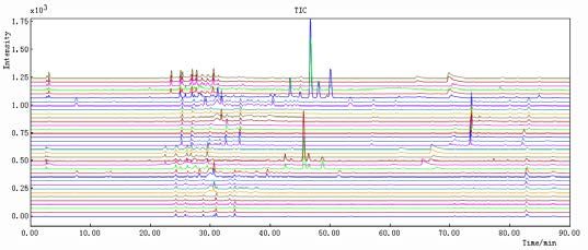
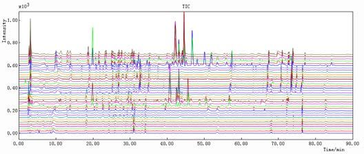
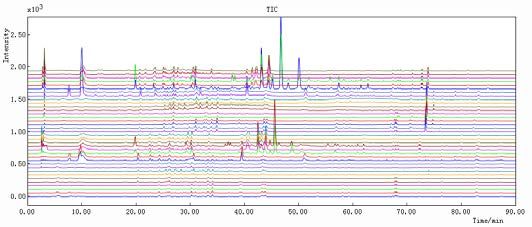
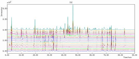
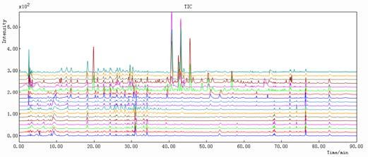
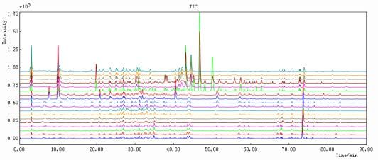
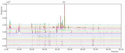
LIST OF FIGURES

Figure 1. Dendrobium fresh(left) [22] and Dendrobium dry stems (right) [23] ......... 11
Figure 2. Basic flavonoid structure [27] ..................................................................... 13
Figure 3. Schematic representation of HPLC system [47].......................................... 15
Figure 4. Schematic representation of a Diode Array Detector (DAD) [48] .............. 16
Figure 5. Schematic representation of PCA [54] ........................................................ 18
Figure 6. Decomposition of and matrices in PLS components [55] .................... 20
Figure 7. Chromatographic fingerprints simulated with different separation degrees
[60] ............................................................................................................................... 23
Figure 8. Simplicity (A), peak factor (B) and warping effect (C) values for all
combinations of segment length and slack size using simulated data. For plots (A) and
(B) a value close to one indicates that data are well aligned and that the area has
changed insignificantly, respectively. For plot (C) a value close to two means that
peaks are both aligned and that the change in the area is minimal. The white triangle
in the upper left corner contains unfeasible combinations of segment length and slack
size in the COW algorithm. [75] .................................................................................. 34
Figure 9. Map of People’s Republic of China [83] .................................................... 38
Figure 10. HPLC-DAD Dionex Ultimate 3000 LC System used in CSU and in UiB
[84] ............................................................................................................................... 39
Figure 11. Results obtained in Norway: from 1-12 DO samples and from 13-18 D
samples. Results were obtained at (A) 254 nm, (B) 280 nm, (C) 310 nm and (D) 335
nm ................................................................................................................................ 44
Figure 12. Results obtained in China: from 1-12 DO samples and from 13-18 D
samples. Results were obtained at (A) 254 nm, (B) 280 nm, (C) 310 nm and (D) 335
nm ................................................................................................................................ 45
Figure 13. Results obtained in Norway: 1-12 DO samples and 13-18 D samples.
Results obtained in China: 19-30 DO samples and 31-36 D samples. All the results
were obtained at (A) 254 nm, (B) 280 nm, (C) 310 nm and (D) 335 nm .................... 47
Figure 14. Results obtained in UiB at 254 nm. Spectra 1-12 DO and 13-18 D: (A)
before peak alignment and (B) after peak alignment ................................................... 49
Figure 15. Results obtained in CSU at 254 nm. Spectra 1-12 DO and 13-18 D: (A)
before peak alignment and (B) after peak alignment ................................................... 50
Figure 16. Results obtained in UiB and CSU together at 254 nm. Norway: 1-12 DO,
13-18 D and China: 19-30 DO and 31-36 D. (A) before peak alignment and (B) after
peak alignment ............................................................................................................. 51
Figure 17. Results obtained in UiB after adding the 4 wavelengths (254, 280, 310 and
335 nm), 1-12 DO and 13-18 D: (A) before peak alignment and (B) after peak
alignment...................................................................................................................... 53
Figure 18. Results obtained in CSU after adding the 4 wavelengths (254, 280, 310,
335 nm), 1-12 DO and 13-18 D: (A) before peak alignment and (B) after peak
alignment...................................................................................................................... 54

 4
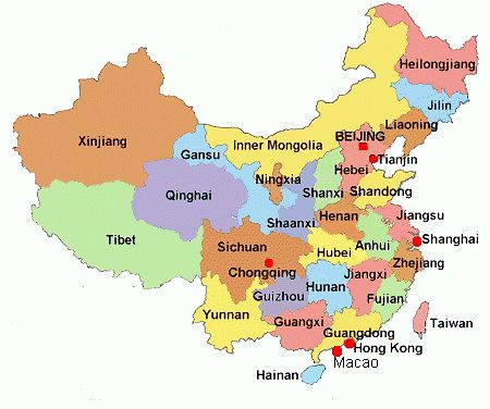
Figure 19. Results obtained in UiB and CSU together after adding the 4 wavelengths
(254, 280, 310 and 335 nm). Norway: 1-12 DO, 13-18 D and China: 19-30 DO, 31-36
D. (A) before peak alignment and (B) after peak alignment ....................................... 55
Figure 20. Results obtained in UiB: (A) before peak alignment with PC1–63.4% and
PC2–12.8%; (B) after peak alignment, reference: sample DO5(1) PC1–69.1 % and
PC2–12.8%. The figures below each score plot represent Loadings vs Variables for
Comp. 1 and Comp.2 ................................................................................................... 59
Figure 21. Results obtained in CSU: (A) before peak alignment PC1–41.0% and
PC2–23.7%; (B) after peak alignment, reference: sample DO4(1) PC1–52.8% and
PC2–14.9%. The figures below each score plot represent Loadings vs Variables for
Comp. 1 and Comp.2 ................................................................................................... 62
Figure 22. Results obtained for UiB and CSU together: (A) before peak alignment
PC1–28.3% and PC2–22.5%; (B) after peak alignment, reference: sample DO2(1)N
PC1–46.6% and PC2–10.7%. Blue color represents Norway, red color represents
China, the squares represent DO samples and the circles represent D samples. The
figures below each score plot represent Loadings vs Variables for Comp. 1 and
Comp.2 ......................................................................................................................... 65
Figure 23. UiB: (A) before peak alignment PC1–42.5% and PC2–29.3%; (B) after
peak alignment, reference: sample DO5(1) PC1–40.5% and PC2–21.7%. The figures
below each score plot represent Loadings vs Variables for Comp. 1 and Comp.2 ..... 68
Figure 24. CSU: before peak alignment PC1–33.4% and PC2–22.8%; (B) after peak
alignment, reference: sample D2N PC1–52.8% and PC2–23.7%. The figures below
each score plot represent Loadings vs Variables for Comp. 1 and Comp.2 ................ 71
Figure 25. CSU and UiB together: (A) before peak alignment PC1–18.8% and PC2–
15.5%; (B) after peak alignment, reference: sample DO4(2)C PC1–23.2% and PC2–
16.9%. Blue color represents Norway, red color represents China, the squares
represent DO samples and the circles represent D samples. The figures below each
score plot represent Loadings vs Variables for Comp. 1 and Comp.2 ........................ 74
Figure 26. PLS-DA score plots of the first two latent variables for samples tested in
CSU after peak alignment. Objects of class -1 (Dendrobii) are labeled in blue and
objects of class 1 (Dendrobii Officinalis) are labeled in red ....................................... 77
Figure 27. Graphic of variables vs Variable selectivity ratio (3.73 as limit) .............. 78
Figure 28. Graphic representation of Predicted (red) and Measured (blue) for Var
10802, SEP = 0.133, Comp. 3...................................................................................... 78

 5
LIST OF TABLES

Table 1 - Information content of simulated chromatographic fingerprints with
different separation degrees represented in Figure 7 [59] ........................................... 23
Table 2 - Orthogonal (Taguchi) L 9 Array Design ....................................................... 24
Table 3 - Description of Dendrobium (D) samples ..................................................... 38
Table 4 - Description of Dendrobium Officinale (DO) samples ................................. 38
Table 5 - 34-2 Fractional Factorial Design 4 and respective results obtained for
information content relative to the spectra obtained at 254 nm ................................... 41
Table 6 - Summary of PCA results before (*) and after (**) peak alignment ............ 75
Table 7 - Results obtained for UiB and CSU when one wavelength was used, before
(*) and after (**) peak alignment................................................................................. 79
Table 8 - Results obtained for UiB and CSU when four wavelengths were used,
before (*) and after (**) peak alignment ..................................................................... 80

 6
LIST OF ABBREVIATIONS, ACRONYMS AND TERMINOLOGY

airPLS adaptive iteratively reweighted Penalized Least Squares
COW Correlation optimized warping
CSU Central South University
D Dendrobii
DAD Diode-Array Detector
DO Dendrobii Officinalis
GC-MS Gas Chromatography coupled with Mass spectrometry
HM Herbal Medicine(s)
HPLC-DAD High-Performance Liquid Chromatography coupled
 with Diode-Array Detector
HPLC-MS High-Performance Liquid Chromatography coupled
 with Mass Spectrometry
IUPAC International Union of Pure and Applied Chemistry
LC Liquid Chromatography
LV Latent Variable(s)
MS Mass Spectrometry
PC Principal Component(s)
PCA Principal Component Analysis
PLS Partial Least Squares
PLS-DA Partial Least Squares-discriminant analysis
SEP Standard Error of Prediction
SSE Sum Square Errors
SVD Singular Value Decomposition
UiB University of Bergen

 7
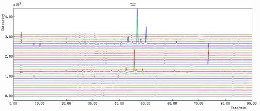
ABSTRACT

The fingerprinting quantitative analysis combining similarity evaluation, Principal
Component Analysis (PCA) and Partial Least Squares Discriminant Analysis (PLS-
DA) is a valid method for classification of herbal medicine species. The main
objective of this study was to investigate the chemical differences between two
officinal Chinese pharmacopoeia species Dendrobii Caulis (Shihu) and Dendrobii
Officinalis Caulis (Tiepi Shihu). As far as is known no systematic chemical
differences study between the two species, especially based on Dendrobii whole
profile, was done before. A total of twelve samples, six from each species collected
from five different provinces in China were analyzed in China at Central South
University (CSU) and in Norway at University of Bergen (UiB). The extraction
method of flavonoids or other phenolic compounds present in the two different
species of Dendrobii and the sample preparation were developed and were relatively
simple processes. The main advantages of these processes were low solvent
consumption, relatively short extraction time, good extraction efficiency, stability and
repetitiveness. The HPLC-DAD method was developed to separate the components
present in the two species of the Chinese herbal medicine (HM) Dendrobii with good
resolution. Based on the optimization of the chromatography conditions, an efficient
chromatography fingerprint of these species was established. It was verified that some
compounds with retention times in the range from 40 to 50 min appeared in Dendrobii
species but not in Dendrobii Officinalis species. All the samples were analyzed at four
different wavelengths, the results obtained at 254 nm being the most useful. PCA
results showed that the distribution of the samples in two groupings before and after
peak alignment is almost the same revealing the similarity between the two species.
Regarding PLS results, it was observed a regular relationship between the Dendrobii
samples and between the Dendrobii Officinalis samples with a clear separation
between the two different clusters. In the results obtained for one wavelength or even
four wavelengths, the final predictive properties of the models were good due to the
low values obtained for the Standard Error of Prediction (SEP). The selectivity ratio
showed specific regions in the raw data that could help distinguish between the two
Dendrobii species. The method established by this study could be applied to other
similar Dendrobii species for the quality assessment.

 8
1. INTRODUCTION

1.1 Theory and Background

A great number of oriental countries have extensively used traditional HM and their
preparations for many centuries [1, 2].

The quality control of traditional HM is one of the main concerns for its application
and development, so to obtain additional evidence of its safety and efficacy more
scientific research and improvement of the quality of the research is needed. This fact
is recognized by World Health Organization: “Despite its existence and continued use
over many centuries, and its popularity and extensive use during the last decade,
traditional medicine has not been officially recognized in most countries.
Consequently, education, training and research in this area have not been accorded
due attention and support. The quantity and quality of the safety and efficacy data on
traditional medicine are far from sufficient to meet the criteria needed to support its
use worldwide. The reasons for the lack of research data are due not only to health
care policies, but also to a lack of adequate or accepted research methodology for
evaluating traditional medicine” [3].

1.1.1 Chromatographic Fingerprints and Quality Control of Herbal
Medicines

A chromatographic fingerprint of a HM is, by definition, “a chromatographic pattern
of the extract of some common chemical components of pharmacologically active and
or chemically characteristics [1, 4-6]. This chromatographic profile should be featured
by the fundamental attributions of ‘integrity’ and ‘fuzziness’ or ‘sameness’ and
‘differences’ so as to chemically represent the HM investigated” [1, 6, 7]. So, using
the chromatographic fingerprints it is possible to do accurately the authentication and
identification of the HM (‘integrity’) even if the concentration/amount of the
characteristic constituents are slightly different for the same HM (‘fuzziness’) and the

 9
chromatographic fingerprints can also effectively show the ‘sameness’ and the
‘differences’ between several samples [1, 6, 8].

In every HM and its extract there is a great number of components that are unknown
and most of them are in low amount and even in the same HM samples it is frequently
observed some variability [1, 9, 10]. Therefore, to obtain a chromatographic
fingerprint that represents the pharmacologically active and chemically characteristic
constituents is not very simple [1].

To ensure the consistency of HM products, the phytoequivalence concept was
developed. The full HM product can be seen as the active compound, because the
several constituents act together being responsible for its therapeutic effect.
According to the phytoequivalence concept, “a chemical profile, such as a
chromatographic fingerprint, for an herbal product should be constructed and
compared with the profile of a clinically proven reference product” [1, 11].

So, an extract of the HM should be prepared and its activity by pharmacological and
clinical methods should be determined. A qualitative and quantitative profile of all the
constituents should be obtained by using a hyphenated technique with high efficiency
and sensitive detection, such as HPLC-DAD, HPLC-MS or GC-MS. These
hyphenated techniques used to obtain the chromatographic fingerprints and further
combined with chemometric approaches are the perfect tools for quality control and
authenticity of HM [1, 2, 11].

To obtain a good chromatographic fingerprint that represents the phytoequivalence of
a HM depends on many factors, such as extraction methods, measurement instruments,
measurement conditions, etc. The chemical constituents in the HM may also vary
depending on plant origins, harvest seasons, drying processes and even possible
contaminations such as excessive or banned pesticides, microbial contaminants, heavy
metals, chemical toxins, etc. [1, 2, 12].

Since a single HM may contain a great number of natural constituents, obtaining a
good fingerprint is dependent on the method of extraction and the sample preparation.

A powerful tool for the quality control of herbal medicines is the combination of
chromatographic fingerprints of HM with chemometric approaches.

 10
In quality control of herbal medicines, the research field is very interdisciplinary
because it uses knowledge from chemistry, biochemistry, pharmacology, medicine
and also statistics [1, 2].

1.1.2 Herbal Medicine Dendrobii

The second largest group of the family Orchidaceae is the genus Dendrobii or
Dendrobium, which comprises approximately 1400 species [13, 14].

In Pharmacopoeia of the People’s Republic of China 2005 edition also known as the
Chinese Pharmacopoeia 2005, Dendrobii Caulis – Shihu – is officially recorded as the
fresh or dried stem of Dendrobium nobile Lindl, Dendrobium officinale Kimura et
Migo, Dendrobium fimbriatum Hook. var. oculatum Hook and similar species [15].

In Chinese history and literature, Dendrobii Officinale Kimura et Migo was described
as a miraculous drug. Its antitumor [16], cardio-protective [17, 18],
immunomodulatory [19] and hepatoprotective [20] effects have recently been
confirmed by modern research. Recently, in the Chinese herbal medicine market, the
price of Dendrobium officinale Kimura et Migo has increased one hundred times
more in relation to other Dendrobii species. Dendrobium officinale Kimura et Migo is
even considered the precious wild “Tiepi Shihu” in traditional conception and due to
the increasing demand and price is often adulterated by other related species [21].

 Figure 1. Dendrobium fresh(left) [22] and Dendrobium dry stems (right) [23]

 11
Therefore, in current Chinese Pharmacopoeia 2010, Dendrobii Officinalis Caulis
(Tiepi Shihu) is separated from Dendrobii Caulis (Shihu) and recorded as the dried
stem of Dendrobium officinale Kimura et Migo, while Dendrobii Caulis (Shihu) is
officially recorded as the fresh or dried stem of Dendrobium nobile Lindl.,
Dendrobium chrysotoxum Lindl. and Dendrobium fimbriatum Hook. [24]. However,
from the data base of Chinese State Food and Drug Administration for registered
medicines entitled with “Shihu” and produced by more than 190 factories, no species
designation was clarified [25].

And to the best of our knowledge, no systematic chemical differences study,
especially based on Dendrobii whole profile, between the two species has been done.

1.1.2.1 Flavonoids and Herbal Medicine Dendrobii

Flavonoids are phenolic compounds widely present in an extensive range of natural
plants, with over 8000 individual substances known. The flavonoids are classified as
flavones, flavanones, catechins and anthocyanins. The basic structure of flavonoids is
shown in Figure 2. These type of compounds show different functions in plants, such
as antioxidants, antimicrobials, photoreceptors, visual attractors, feeding repellants,
and light screening. Studies on pharmacological effects of flavonoids have shown that
these compounds have extensive biological activities and significant pharmacological
effects on cardiovascular, digestive and nervous systems. They also have anti-
inflammatory, antiallergenic, antiviral, vasodilatory, immunoregulator, anti-tumor,
analgesic, liver-protecting, aging-delaying, antidepressive and immunity-improving
effects [26-28]. The role of flavonoids as antioxidants that reduce free radical
formation and quench free radicals has been the subject of many studies. The
antioxidant activity is observed in both the absorbed flavonoids and their metabolites.
It is very common that the flavonoids occur in plants as glycosylated derivatives and
they also give a contribution to the colors in leaves, flowers, and fruits [29].
Significant sources of flavonoids are the medicinal plants and their phytomedicines
[27, 30].

 12
Figure 2. Basic flavonoid structure [27]

It is convenient to use dry, lyophilized or frozen samples because when the plant
material to be analyzed is fresh or non-dried, the flavonoids (especially glycosides)
can be decomposed by enzymatic action. Therefore, the dry samples are grinded into
a powder and the extraction solvent is selected according to the polarity of the
flavonoids present in the sample to be analyzed. For less polar flavonoids such as
isoflavones, flavanones, flavonols and methylated flavones the extraction is done with
chloroform, dichloromethane, diethyl ether or ethyl acetate whereas more polar
aglycones and flavonoid glycosides are extracted with alcohols or alcohol–water
mixtures. Direct solvent extraction is still the most used method [31]. This kind of
medicinal material is usually extracted using ultrasonic methods and with alcohols
[32-34] and also in order to remove saccharides since they are not soluble in this type
of solvents [35, 36].

The application of standardized UV/UV–Vis spectroscopy has been applied for years
in the analyses of this kind of polyphenolic compounds. This type of compounds has
two characteristic UV absorption bands, with maxima within an interval that varies
from 240 to 285 and from 300 to 550 nm.

It is possible to recognize the different flavonoid classes by their UV spectra
characteristics that include the effects of the number of aglycone hydroxyl groups,
glycosidic substitution pattern and the nature of aromatic acyl groups [31, 37].

The type of flavonoids existent in Dendrobium species are anthocyanins
(anthocyanidins), flavonol glycosides (based on kaempferol, quercetin, myricetin and
methylated derivatives) and flavonol aglycones [38-43].

 13
1.1.3 Analytical techniques Chromatography is defined by International Union of Pure and Applied Chemistry (IUPAC) as “a physical method of separation in which the components to be separated are distributed between two phases, one of which is stationary (stationary phase) while the other (the mobile phase) moves in a definite direction.” Liquid Chromatography (LC) is also defined by IUPAC as “A separation technique in which the mobile phase is a liquid. LC can be carried out either in a column or on a plane. Present-day liquid chromatography generally utilizing very small particles and a relatively high inlet pressure is often characterized by the term high-performance or high-pressure liquid chromatography, and the acronym HPLC” [44]. The hyphenated analytical technique used in this work, both in China and Norway, was High-Performance Liquid Chromatography with Diode-Array Detection (HPLC- DAD). 1.1.3.1 HPLC-DAD High-performance (or High-pressure) Liquid Chromatography As mentioned before, the mobile and stationary phases are the two parameters related to the separation that is carried out in a chromatographic system. In HPLC, the stationary phase is packed into a column capable to support high pressures while the mobile phase is a liquid supplied under high pressure (up to 400 bar/ 4 × 10⁷ Pa) to guarantee a constant flow rate and consequently reproducible chromatography. Therefore, the sample is dissolved in the mobile phase and after it is forced to pass through the stationary phase by means of high pressure so that chromatographic separation occurs because the different components of the sample have different affinity with the stationary or the mobile phase and consequently take different times 14
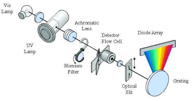
to move from the position of sample introduction to the position where they are detected. With previous knowledge about the analytes under investigation it is possible to change the properties of the stationary and/or mobile phases to achieve the desired separation. Different kinds of detectors can be coupled to HPLC and its type is chosen according to the sort of analysis being performed, for instance qualitative (identification) or quantitative [2, 45, 46]. The HPLC system is schematized in Figure 3. Figure 3. Schematic representation of HPLC system [47] Diode Array Detector (DAD) A detector is a device that is used to sense each solute as it is eluted from a chromatography column. The diode array detector can use a deuterium or xenon lamp that emits light over the UV spectrum range or a tungsten lamp for the visible region. The light from the lamp is focused by a lens through the sample cell and onto a holographic grating. Therefore, the sample is subjected to light of all wavelengths produced by the lamp. The dispersed light from the grating is able to reach a diode array. The array can have many hundreds of diodes and the output from each diode is regularly sampled and 15
stored in a computer. At the end of the run, it is possible to select the output from any
diode and to produce a chromatogram using the UV wavelength that was falling on
that particular diode [46].

The diode array detector is schematized in Figure 4.

 Figure 4. Schematic representation of a Diode Array Detector (DAD) [48]

This analytical technique HPLC-DAD was previously used in the analysis of
Dendrobium species, as was HPLC coupled with Mass Spectrometry (MS), an
extremely versatile technique when it comes to analyze this kind of samples [49-53].

1.1.4 Chemometric techniques

With the use of chromatographic instrumentation two goals can be achieved, such as
quantitative analysis and qualitative (identification) analysis. In quantitative analysis
it is possible to determine how much of a substance is present in a mixture and the
data is obtained from peak height or peak area measurements. In qualitative analysis
the solutes present in a mixture can be identified and the data is often obtained from
retention measurements [46].

Pattern recognition tools as Principal Component Analysis (PCA) and Partial Least
Squares Discriminant Analysis (PLS-DA) are very useful and widely used
chemometric techniques to visualize and summarize the very large amount of data
obtained from multivariate measurements in chemistry. By using the proper

 16
mathematical approaches, pattern recognition is used to identify patterns in large data
sets [54].

1.1.4.1 Principal Component Analysis

In chromatography, very often the chromatographic peaks are partially overlapping,
so chemometric methods help to resolve the chromatogram into individual
components. In order to obtain predictions, first the chromatogram is treated as a
multivariate data matrix and then PCA is performed. In the mixture, each compound
is a (chemical) factor with its spectra and elution profile which by a mathematical
transformation can be related to principal components. After performing PCA, there is
a reduction of the original variables to a number of significant principal components
(e.g. two). In this way, PCA is used as a form of variable reduction, reducing the large
original dataset to a much smaller manageable dataset more easily interpreted [54].

In the case of coupled chromatography like HPLC-DAD, the essential dataset for a
single chromatogram can be described as a sum of responses for each significant
compound in the data, characterized by an elution profile and a spectrum plus noise or
instrumental error. Using matrix notation it can be written as:

 = +

 Equation 1

where is the original data matrix or coupled chromatogram, is a matrix consisting
of the elution profiles of each compound, is a matrix consisting of the spectra of
each compound and is an error matrix.

In summary, PCA is a way of identifying patterns in data and expressing it in a way to
emphasize their differences and similarities. Since patterns in data of high dimension
can be hard to find and where graphical representation is not available, PCA is a
powerful tool for analyzing data. Another advantage of PCA is that there is not much
loss of information once the patterns are found in the data and this data is compressed
by reducing dimensions [54].

 17
Scores and Loadings The abstract mathematical transformation of the original data matrix in PCA is: = + Equation 2 where are called scores, and have as many rows as the original data matrix, are the loadings, and have as many columns as the original data matrix and the number of columns in the matrix T equals the number of rows in the matrix P. The principal components are vectors of loadings or scores where variables or objects with largest variance will make the greatest impact. The scores, in the case of chromatography, relate to elution profiles and the loadings relate to the spectra. The schematic representation of PCA is showed in Figure 5. Figure 5. Schematic representation of PCA [54] The aim of PCA is to obtain a description of a data table in terms of uncorrelated new variables called principal components (PCs). The PCs are linear combinations of all the original variables subjected to two restrictions: First they are located in the direction explaining most of the variation in the data table and second they are 18
orthogonal with respect to each other (angle between them is 90°) and to the residual
matrix.

As said before, the PCs are given as vectors of loadings or scores. The loading vectors
represent a basis for the variable space, while the score vectors represent a basis for
the object space. Plotting the objects on the loading vectors shows the relationships
between objects, while plotting the variables on the score vectors shows the
relationships between variables.

The significance of a PC is measured through the ratio of its variance to the total
variance contained in the original variables. A PC with small variance usually means
that it carries little information. The variance explained is most often used as the
criterion for deciding on the number of PCs needed to obtain a data table [54].

1.1.4.2 Partial Least Squares

Partial Least Squares Regression (PLS) is a calibration method based on finding the
model relating the components of to the components in . PLS components are
calculated finding the directions of maximum covariance between and , i.e., the
maximum variation of correlated to . PLS Component is different from the PCA
component that means the scores obtained in PLS are different from the ones obtained
in PCA. In PLS1 a single variable is predicted and in PLS2 a block of variables is
predicted.

In Figure 6 it is represented the decomposition of ( , ) and ( , ) matrices in
PLS components. After, the construction of the regression model = ( and
matrices are represented by their components) is done.

 19
Figure 6. Decomposition of and matrices in PLS components [55]

In the calibration step, PLS components and regression vectors are calculated
sequentially. There is the decomposition of and in components and the
calculation of the regression coefficient.

In the prediction step, first there is the Calculation of scores related to the response of
new samples, :

 =

 Equation 3

After the prediction of Y scores for the new samples ( ):

 =

 Equation 4

And finally, the calculation of the properties of interest ( ) for the new samples
using the calculated scores:

 =

 Equation 5

In summary, building a PLS model includes several steps such as: Preprocessing data
sets if required ( and ): in the calibration set or in the validation set and in the new
unknown samples; Selection of the size of the calibration model (number of
components); Exploration of and data sets and their relationship: study of
variance explained by the model and outlier detection and elimination from the

 20
calibration set; Qualitative interpretation of the model; Model validation and finally
Prediction of new samples [55].

Partial Least Squares Discriminant Analysis (PLS-DA) is a classical PLS regression,
with a regression mode, where the response variable indicates the classes (or
categories) of the samples. PLS-DA has often been used for supervised classification,
i.e., classification and discrimination problems. The response vector is qualitative and
is recoded as a dummy block matrix where each of the response categories is coded
with an indicator variable. After this, PLS-DA is performed as if the response vector
was a continuous matrix [54].

Classification problems in fingerprints data analysis are complex due to the many
variables and few samples/objects issue. This makes that many solutions can be found
to separate the classes. The PLS-DA score plots as showed in most classification
applications present an overoptimistic view of the separation between the classes.

Even using PLS-DA to discriminate a random data set into two groups does almost
always give a PLS score plot with perfect separation between the two arbitrary classes.

The permutation testing and cross model validation are used to assess the validation
of classification models. Permutation tests show that when cross validation is not
applied appropriately, it leads also to overoptimistic results [56].

Selectivity ratio can be used to detect marker candidates and can be defined for each
variable as:

 = , / , = 1,2,3, ..

 Equation 6

where is the explained variance and the residual variance. Based on an F-
test, this is a valuable property for variable selection especially when the ratio of the
number of variables to the number of objects is high [57].

 21
PCA and PLS diverge in the optimization problem they solve to find a projection
matrix but they are both linear decomposition techniques and they can be combined
with various functions.

The statistical measure of the multivariate distance of each observation from the
center of the data set is named Hotelling's T-squared statistic. To calculate the T-
squared statistic, PCA uses the main principal components and it is used for the
detection of outliers [58].

1.1.5 Information theory applied to chromatographic fingerprint of HM

Information theory is used to evaluate the chromatographic fingerprints. Since the
chromatographic fingerprint obtained is deeply dependent on the chromatographic
separation degree and concentration distribution of each chemical component, based
on the information content it is possible to select the chromatographic fingerprint with
the best separation degree and the most uniform distribution of the chemical
compounds.

A chromatographic fingerprint may be considered as a continuous signal determined
by its shape and according to Ref. [59], the information content of a continuous signal
can be defined as:

 Ф= − ∫

 Equation 7

where is the chromatographic response of all chemical components present in the
fingerprint under investigation.

The evaluation of the quality of the HM is done based on similarities and/or
differences of the chromatographic shapes and based on the separation degree of each
chemical component between the fingerprints obtained for the different HM under
study.

Therefore, first a chromatographic fingerprint is normalized with its overall peak area
equal to one and after its information content is obtained based on Equation 8 [60]:

 22
Ф= − ∫ ⁄[ ( )] ⁄[ ( )]

 Equation 8

Two advantages of calculating the information content according to Equation 8 is
that the whole chromatogram is taken into account and also that the noise should have
a small influence in this calculation.

Figure 7 shows four simulated chromatographic fingerprints with different separation
degrees (a, b, c and d). The concentration distributions of the four peaks are the same.
The values of the chromatographic resolution ( ) are displayed in Table 1. The
results suggest that the further chromatographic separation from Fig. 7a to Fig. 7d (R s
from 1.50 to 2.00), which can not cause any addition to the information content Ф, is
unnecessary. However, the serious overlapping situation in Fig. 7b and Fig.7c
(R s =0.63, 0.31) causes a loss of the information content [60].

 Figure 7. Chromatographic fingerprints simulated with different separation degrees [60]

Table 1 - Information content of simulated chromatographic fingerprints with different separation degrees
represented in Figure 7 [60]

 Data a b c d
 Rs 1.50 0.63 0.31 2.00
 Ф 6.04 5.50 4.83 6.04

 23
1.1.6 Orthogonal (Taguchi) “L” Array Design

Genichi Taguchi (Japan) developed a method for designing experiments to investigate
how different parameters affect the mean and variance of a process performance
characteristic that defines how well the process is functioning. This experimental
design involves the use of orthogonal arrays to organize the parameters affecting the
process and the levels at which they should be varied.

The Taguchi method tests pairs of combinations instead of testing all possible
combinations like in factorial design. With this method it is possible to determine
which factors most affect product quality with a minimum amount of experimentation,
consequently saving resources and time. The method works better for an intermediate
number of variables (3 to 50), few interactions between variables and when only few
variables contribute significantly.

There are five general steps involved in the Taguchi Method Design of Experiments:

 - Define a target value to measure the performance of the process;
 - Determine the parameters that affect the process;
 - Construct the orthogonal array for the parameter design showing each
 experiment number and conditions;
 - Carry on the experiments indicated in the completed array to collect the data;
 - Data analysis in order to check the effect of each parameter on the
 performance measure.

In Table 2 it is represented a 34-2 Fractional Factorial Design 4, with Factors at three
Levels (9 runs), where P1, P2, P3 and P4 are the parameters that can affect the
process.

 Table 2 - Orthogonal (Taguchi) L 9 Array Design

 Experiment P1 P2 P3 P4 IC
 1 1 1 1 1 IC1
 2 1 2 2 2 IC2
 3 1 3 3 3 IC3
 4 2 1 2 3 IC4
 5 2 2 3 1 IC5
 6 2 3 1 2 IC6
 7 3 1 3 2 IC7
 8 3 2 1 3 IC8
 9 3 3 2 1 IC9

 24
After calculating the information content for each experiment, the average
information content value ( ) is calculated for each factor and level. This is done
according to Equation 9, where is the level number (1, 2 or 3) and is the parameter
number (1, 2, 3 or 4).

 ∑
 , =
 3

 Equation 9

The range R ( = ℎ ℎ − ) of the for each parameter is calculated and the
larger R value for a parameter means a larger effect of the variable on the process [61,
62].

1.1.6.1 Advantages and Disadvantages of "L" Array Design

The advantage of the Taguchi method is that emphasizes a mean performance
characteristic value close to the target values and it allows the analysis of many
different parameters without a high amount of experimentation. It obtains a lot of
information about the main effects in a relatively few number of runs. It allows the
identification of key parameters that have the most effect on the performance
characteristic value so that further experimentation on these parameters can be
performed and the parameters that have little effect can be ignored.

The main disadvantage of this method is that the results obtained are only relative.
Also, since the orthogonal arrays do not test all variable combinations, this method
should not be used when all relationships between all variables are needed. The
Taguchi method provides limited information about interactions between parameters
[61, 62].

 25
1.1.7 Pre-processing of data

Prior to chemometric analysis of the chromatographic results using MATLAB and
Sirius, it is necessary to pre-treat the chromatograms obtained. There are some pre-
processing steps that seem particularly important for the further analysis of the HPLC-
DAD data. First, the pre-processing of data done using the Changde program included
three processes; namely data smoothing and differentiation and baseline correction.
After this, alignment of the chromatographic data is also needed since no internal
standard is used during the experiments. And finally, the data obtained was also
normalized.

After the pre-processing of fingerprints it is possible to proceed to the chemometric
analysis of the data obtained.

1.1.7.1 Data smoothing and differentiation

The aim of data smoothing and differentiation is to remove the random errors from
the quantitative information. Disregarding the source of these errors, they are usually
described as noise and it is very important to remove as much as possible this noise
without losing the basic information.

For this purpose, the method of least squares is used, where the set of points is fitted
to some curve and it is assumed that all the error is in the ordinate ( ) and not in the
abscissa ( ). The least squares minimize the sum of squared residuals, where a
residual is the difference between an observed value and the fitted value provided by a
model.

Using averaging prior to smoothing, it is possible to reduce the noise nearly as the
square root of the number of points that were used.

Thereby, this function known as Savitzky-Golay filter for smoothing and
differentiation will act as a filter to smooth noise fluctuations and avoid distortions
into the dataset [63].

 26
1.1.7.2 Baseline correction

Signals of analytical instruments like chromatography essentially contain chemical
information, baseline and random noise.

For the baseline correction an algorithm named adaptive iteratively reweighted
Penalized Least Squares (airPLS) was used. This method iteratively changes weights
of sum squares errors (SSE) between the fitted baseline and the observed signals. The
weights of the SSE are adaptively obtained using the difference between the
previously fitted baseline and the observed signals [64].

The airPLS leads to a balance between fidelity to the observed data and the roughness
of the fitted data.

In Equation 10, is the vector of the analytical signal and is the fitted vector and
is the length of both of them. The fidelity of to can be expressed as the sum square
errors between them.

 = �( − )2
 =1

 Equation 10

Balance between fidelity and smoothness is measured as the fidelity plus penalties on
the roughness. It can be given by Equation 11, where is the derivative of the
identity matrix such that = ∆ .

 = + = ‖ − ‖2 + ‖ ‖2

 Equation 11

Although adaptive iteratively reweighted procedure is similar to the weighted least
squares and to iteratively reweighted least squares [65, 66, 67], it calculates the
weights in different ways and adds a penalty item to control the smoothness of the
fitted baseline. Each step of this proposed procedure involves calculating a weighted
penalized least squares according to Equation 12, where is the weight vector and
represents each iterative step.

 27
 2

 = � | − |2 + �� − −1

 �
 =1 =2

 Equation 12

So, airPLs algorithm can be applied to chromatograms since it gives extremely fast
and accurate baseline corrected signals for both fitted and observed signals [64].

1.1.7.3 Automated alignment of chromatographic data

The datasets must be preprocessed before PCA and PLS-DA analysis in a way that the
elements in the matrix for individual samples describe the same phenomena. For peak
alignment in chromatographic data, several types of approaches have been developed.
In some approaches, the retention time shifts have been corrected by making internal
standards added or making marker peaks coincide in all chromatograms under study
[68-74].

For the peak alignment in this work, automated alignment of chromatographic data
was used, where the data is preprocessed in order to correct unwanted time-shifts.
This approach includes the selection of a reference sample to warp towards. This
selection procedure is used when there are no internal standards available or
normalization to correct the signal. This method is used for datasets obtained from
quite homogeneous samples with very similar chromatographic profiles [1, 75].

1.1.7.3.1 Correlation optimized warping (COW)

The COW algorithm, introduced by Nielsen et al. [76] is a method to correct shifts in
discrete data signals. This algorithm, that it is assumed to preserve the properties of
peak shape and area, aligns a sample chromatogram (digitized vector) towards a
reference chromatogram (reference sample vector). This reference sample is used to
align the entire data set.

 28
The COW algorithm requires two user input parameters that are typically selected on
a trial and error basis by visual inspection of the chromatographic profiles: the
segment length and the slack size (flexibility).

A slightly modified version of COW algorithm developed by Tomasi et al. [77] is
used here and the main change regards the sharing of the boundaries between adjacent
segments. In this new version of COW, the correlation coefficient between two
vectors and of length is calculated as:

 ( , )
 ( , ) =
 � ( ) ( )

 [( − −1 ) ] ( − –1 ) �

 = =
 �‖2 (‖ ‖22 − �)1/2
 ‖ ‖
 �‖2 (‖ ‖2 − �)1/2

 Equation 13

Where � represents the centered , � is the mean of and the centering matrix
 − −1 is symmetric and idempotent [75].

1.1.7.3.2 Reference chromatogram selection

The reference chromatogram (sample) should be as representative as possible for all
phenomena of interest in the data set.

This method is based on the product of the correlation coefficients between all
individual chromatograms.

For a given chromatogram , the similarity index (0 < ≤ 1) can
be calculated as follows:

 = �| ( , )|
 =1

 Equation 14

 29
where ( , ) is the conventional correlation coefficient between two
chromatograms in the dataset calculated as shown in Equation 13.

So, the chromatogram with the highest similarity index is selected to be the reference
chromatogram to use with the given dataset [75].

1.1.7.3.3 Simplicity value

The simplicity value is used to measure the alignment of a set of chromatograms
towards the reference chromatogram. Its principle is related to the properties of
singular value decomposition (SVD), where the size of the squared singular values is
directly associated to the sum of squares of the data matrix. Any data matrix, X
(uncentered) can be decomposed as = , where is a diagonal matrix
containing the singular values equal to the square roots of the eigenvalues of .
and are both orthogonal matrices, where the columns in are the eigenvectors of
 and the columns of are the eigenvectors of .

The sum of the first R squared singular values determines how much of the variation
is explained by the corresponding R components:

 2

 ⎛ ⎞
 = � ⎜ ⎛ ⎞
 ⎟

 =1 �∑ =1 ∑ =1 ( , )2
 ⎝ ⎠
 ⎝ ⎠

 Equation 15

where SVD (M) indicates the single value for a given component r and where the data
is scaled to a total sum of squares of one.

Though, to find the optimal combination of segment and slack size as the simplicity
value (0 ≤ simplicity≤ 1), the principle of simplicity is adapted from Henrion &
Andersson [78], Christensen et al. [79] and Johnson et al. [80]:

 30
4

 ⎛ ⎞
 = � ⎜ ⎛ ⎞
 ⎟

 =1 �∑ =1 ∑ =1 ( , )2
 ⎝ ⎠
 ⎝ ⎠

 Equation 16

It is possible to achieve high simplicity values in COW alignment with some
combinations of segment and slack parameters. This is shown in Figure 8 (A) using
simulated data.

This method is focused on preserving total area of all peaks in the chromatographic
profiles and any change introduced by the alignment procedure is not desired. So, a
second criterion that takes into account this area effect has to be included [75].

1.1.7.3.4 The peak factor

The data should be quite homogeneous so that peak area and shape can be the same
before and after alignment. Even if the reference chromatogram is carefully selected a
change in peak area and shape can still occurs. This change can be quantified by the
peak factor, which is a number between 0 and 1.

 ∑ =1(1 − ( ( ), 1)2 )
 =

 Equation 17

 ‖ ( )‖−‖ ( )‖
where, ( ) = � ‖ ( )‖
 � and ‖ ( )‖ = �∑ =1 ( , )2 is the Euclidean length

or norm for ; is the chromatogram before warping while ( ) is the same
sample after alignment.

Values of peak factor measure are shown in Figure 8 (B) for simulated data. It is
possible to see that some combinations of segment length and slack size give high
simplicity values but low peak factor values, so should not be considered as suitable
alignment parameters.

 31
1.1.7.3.5 The warping effect

The warping effect combines simplicity and peak factor (0 ≤ ≤ 2):

 = +

The simplicity factor and the peak factor have the same influence on the warping
effect value. The relation between these three measures is shown in Figure 8. If the
warping effect has a value closer to two means that peaks are both aligned and that the
change in the area is minimal [75].

1.1.7.3.6 Optimization

The warping effect values are optimized in the form of a discrete-coordinates
simplex-like optimization routine carried out in several steps [81]. The first step is to
establish global search space boundaries from the combination of all segment length
and slack sizes of interest. In the second step, by default a 5×5 sparse search grid is
selected in both the segment and slack direction and then the warping effect for these
25 points is determined (this is done using simulated data as an example with segment
length 10–70 and slack size 1–15). The six best (default choice) combinations,
providing the highest warping effect scores, are selected and used as starting points in
a discrete-coordinates simplex optimization part.

1.1.7.3.7 Defining the optimization space

As shown in Figure 8, the search space for segment lengths includes several possible
choices as long as the slack size (flexibility) is large enough. So, longer segment
lengths require more flexibility to give good alignment. Though, this will always
depend on the chromatographic data available such as datasets obtained from quite
homogeneous samples with very similar chromatographic profiles as explained before.

 32
1.1.7.3.7.1 Segment length and slack size (flexibility)

The rule to select the segment length optimization space is:

 ±
 2

 Equation 18

where is the approximate peak width average at the base over all peaks in the
reference chromatogram. Using this rule, the segment lengths will contain both entire
peaks and peak fragments.

For the slack size search space, the number of data points before and after the first and
the last peak, respectively, should be roughly the same as the peak widths (ensuring
enough flexibility), then a slack size search space ranging from 1 to 15 [75].

The simplicity and optimization routines were freely downloaded from Reference [82].

 33
You can also read