Penetration of interferometric radar signals in Antarctic snow
←
→
Page content transcription
If your browser does not render page correctly, please read the page content below
The Cryosphere, 15, 4399–4419, 2021
https://doi.org/10.5194/tc-15-4399-2021
© Author(s) 2021. This work is distributed under
the Creative Commons Attribution 4.0 License.

Penetration of interferometric radar signals in Antarctic snow
Helmut Rott1,2 , Stefan Scheiblauer1 , Jan Wuite1 , Lukas Krieger3 , Dana Floricioiu3 , Paola Rizzoli4 , Ludivine Libert1 ,
and Thomas Nagler1
1 ENVEO  IT GmbH, Innsbruck, Austria
2 Departmentof Atmospheric and Cryospheric Sciences, University of Innsbruck, Innsbruck, Austria
3 Remote Sensing Technology Institute, DLR, Oberpfaffenhofen, Germany
4 Microwaves and Radar Institute, DLR, Oberpfaffenhofen, Germany

Correspondence: Helmut Rott (helmut.rott@enveo.at)

Received: 30 December 2020 – Discussion started: 19 January 2021
Revised: 9 August 2021 – Accepted: 10 August 2021 – Published: 13 September 2021

Abstract. Synthetic aperture radar interferometry (InSAR) is     ues of the computed elevation bias and the elevation differ-
an efficient technique for mapping the surface elevation and     ence between the TanDEM-X DEMs and the REMA show
its temporal change over glaciers and ice sheets. However,       good agreement, a trend towards overestimation of penetra-
due to the penetration of the SAR signal into snow and ice,      tion is evident for heavily wind-exposed areas with low accu-
the apparent elevation in uncorrected InSAR digital elevation    mulation and towards underestimation for areas with higher
models (DEMs) is displaced versus the actual surface. We         accumulation rates. In both cases deviations from the uni-
studied relations between interferometric radar signals and      form volume structure are the main reason. In the first case
physical snow properties and tested procedures for correcting    the dense sequence of horizontal structures related to inter-
the elevation bias. The work is based on satellite and in situ   nal wind crust, ice layers and density stratification causes in-
data over Union Glacier in the Ellsworth Mountains, West         creased scattering in near-surface layers. In the second case
Antarctica, including interferometric data of the TanDEM-X       the small grain size of the top snow layers causes a downward
mission, topographic data from optical satellite sensors and     shift in the scattering phase centre.
field measurements on snow structure, and stratigraphy un-
dertaken in December 2016. The study area comprises ice-
free surfaces, bare ice, dry snow and firn with a variety of
structural features related to local differences in wind ex-     1   Introduction
posure and snow accumulation. Time series of laser mea-
surements of NASA’s Ice, Cloud and land Elevation Satel-         Digital elevation models (DEMs) derived from across-track
lite (ICESat) and ICESat-2 show steady-state surface topog-      interferometric synthetic aperture radar (InSAR) data are a
raphy. For area-wide elevation reference we use the Refer-       main data source for mapping the surface elevation and its
ence Elevation Model of Antarctica (REMA). The different         temporal change over glaciers and ice sheets. Single-pass In-
elevation data are vertically co-registered on a blue ice area   SAR systems, such as the TanDEM-X (TDM) mission, are
that is not affected by radar signal penetration. Backscatter    of particular interest for this task as they are not affected
simulations with a multilayer radiative transfer model show      by variations in the atmospheric phase delay, ice motion and
large variations for scattering of individual snow layers, but   temporal decorrelation. For the analysis and interpretation of
the vertical backscatter distribution can be approximated by     InSAR elevation over snow and ice, the effects of signal pen-
an exponential function representing uniform absorption and      etration have to be taken into account. The surface inferred
scattering properties. We obtain estimates of the elevation      from uncorrected InSAR elevation data refers to the position
bias by inverting the interferometric volume correlation co-     of the scattering phase centre in the snow–firn medium, re-
efficient (coherence), applying a uniform volume model for       sulting in an elevation bias versus the actual surface (Dall,
describing the vertical loss function. Whereas the mean val-     2007). The position and strength of scattering sources in the
                                                                 snow volume and the absorption and scattering losses are

Published by Copernicus Publications on behalf of the European Geosciences Union.
4400                                           H. Rott et al.: Penetration of interferometric radar signals in Antarctic snow

main factors defining the depth of the phase centre below the       of InSAR products. The work presented in this paper takes
snow surface. Backscatter contributions from sources at dif-        on this open issue, exploring relations between interferomet-
ferent depths within a volume-scattering medium, observed           ric parameters and physical snow properties and investigating
under different incidence angles, are causing decorrelation,        the feasibility of deducing the elevation bias from the inter-
depending on the interferometric baseline and incidence an-         ferometric correlation. The study is based on interferometric
gle (Bamler and Hartl, 1998).                                       data of the TDM mission, data from optical satellite sensors
   Hoen and Zebker (2000, 2001) derived a formulation for           and field measurements undertaken in December 2016 on
estimating the power penetration depth in dry snow from             Union Glacier in the Ellsworth Mountains, Antarctica. Lo-
the interferometric coherence, applying a radiative trans-          gistic support was provided by the private company Antarc-
fer model for estimating spatial decorrelation in a volume          tic Logistics & Expeditions LLC (ALE), which conducts air-
of uniformly distributed and uncorrelated scatterers charac-        craft flights to Union Glacier and operates a field station in
terised by exponential extinction. They applied this formula-       summer. The study area comprises ice-free surfaces, bare ice,
tion to derive the C-band penetration depth for different sites     dry snow and firn, exhibiting a diversity of structural features
in Greenland from the coherence of 3 d repeat-pass InSAR            attributed to local differences in wind exposure and snow ac-
data of the ERS-1 synthetic aperture radar (SAR) mission.           cumulation. Time series of ICESat laser measurements from
Forsberg et al. (2000) and Dall et al. (2001) compared sur-         2003 to 2009 and ICESat-2 data show near-steady-state sur-
face elevation measured by airborne laser altimetry and C-          face topography, facilitating the intercomparison of TDM
band single-pass SAR interferometry on the Geiki ice cap in         and optical elevation data.
Greenland. They report zero InSAR elevation bias for wet               In Sect. 2 we describe the study area, present details on the
snow and an average bias of about 10 m for dry snow and             satellite data, and give an account of the structure and mor-
firn. Dall (2007) studied relations between the InSAR ele-          phology of snow and firn at different sites. Section 3 explains
vation bias and the power penetration depth in uniform vol-         the basic concept relating the elevation bias and interferomet-
umes. He shows that the depth of the mean phase centre in           ric coherence in a uniform random volume. Section 4 deals
a volume-scattering medium is approximately equal to the            with vertical co-registration of the different DEMs, includ-
two-way penetration depth if the latter is smaller than about       ing an analysis of the temporal stability of surface elevation,
10 % of the height of ambiguity (Ha ), the height difference        and describes the observed spatial pattern of the backscatter
for a phase shift of 2π . Fischer et al. (2019a, b, 2020) studied   signals, coherence and elevation bias. Section 5 presents re-
various concepts for characterising and modelling the verti-        sults of the inversion of the volumetric coherence in terms
cal backscatter distribution and retrieving the InSAR pene-         of the InSAR elevation bias and compares the retrieved bias
tration bias in the percolation zone of Greenland based on          with elevation differences between TDM DEMs and optical
airborne polarimetric multi-baseline InSAR data and in situ         data. Section 6 includes the discussion, and Sect. 7 presents
measurements of snow structural properties.                         conclusions. The Appendix shows simulations for vertical
   In recent years single-pass InSAR data of the TDM mis-           backscatter distributions at snow pit sites and compares these
sion were widely applied for mapping surface elevation and          with exponential backscatter functions.
elevation change on glaciers and ice sheets. The TDM mis-
sion employs a bistatic interferometric configuration of the
two satellites TerraSAR-X and TanDEM-X flying in close              2     Study area and data
formation in order to form a single-pass SAR interferometer
(Krieger et al., 2013). Rizzoli et al. (2017b) compared surface     2.1    Surface mass balance and orographic effects
elevation over Greenland measured by NASA’s Ice, Cloud
and land Elevation Satellite (ICESat) laser altimeter with the      Union Glacier flows from the ice divide in the Heritage
TanDEM-X global DEM. They report for frozen snow and                Range, Ellsworth Mountains, down to the Constellation Inlet
firn in the wet snow zone, the lower and upper percolation          on Ronne Ice Shelf. The glacier section immediately down-
zone, and the dry-snow zone mean values of the X-band               stream of the main mountain range is exposed to strong kata-
InSAR penetration bias of 3.7, 3.9, 4.7 and 5.4 m, respec-          batic winds so that bare ice appears on the surface (Fig. 1).
tively. Abdullahi et al. (2019) use a linear regression model       The blue ice area (BIA) has a negative specific surface mass
for estimating the elevation bias in TDM DEMs of north-             balance, bn , on the order of several centimetres water equiva-
ern Greenland. The model is based on empirical relations            lent (w.e.) per year due to sublimation (Rivera et al., 2014). In
between coherence and backscatter intensity with the differ-        the BIA an ice runway for landing heavy airplanes on wheels
ence between the uncorrected TDM DEMs and airborne laser            is maintained from November to March. The ALE camp is
altimeter surface heights.                                          located 8 km downstream of the ice runway.
   The complex layered structure of polar snow and firn has a          GPS measurements at stakes, performed during the period
major impact on radar signal propagation and interferometric        2007 to 2011, show ice velocities on the order of 20 m a−1
coherence, an obstacle for establishing a generally applica-        at the glacier gate across the runway (Rivera et al., 2010,
ble, physically based method for estimating the elevation bias      2014). For 2008 to 2012 a mean wind speed of 16.3 knots

The Cryosphere, 15, 4399–4419, 2021                                                     https://doi.org/10.5194/tc-15-4399-2021
H. Rott et al.: Penetration of interferometric radar signals in Antarctic snow                                                  4401

Figure 1. Landsat 8 image acquired on 6 December 2016 (composite of bands 5, 4, 2) with ICESat tracks. Points: elevation difference 1h
(ICESat minus TDM global DEM), colour-coded from 1h = −8 to +4 m. P1 to P5: locations of snow pits. A: ALE camp; BIA: blue ice
area; M: recording meteorological station; S: ice-free slope. The arrow points to the landing strip.

with predominant direction from the south-west (blowing              cantly along this track, even within short distances. For ex-
downstream along the main glacier) was measured at an au-            ample, a radargram along a 6 km transect extending from
tomatic station close to the runway. Wind speed and direc-           the confluence with Driscoll Glacier across Union Glacier
tion are very consistent. Rivera et al. (2014) report a mean         towards the camp shows thickness values of the snow–firn
bn of −0.10 m w.e. a−1 measured at 29 stakes in the BIA              layer ranging from zero on blue ice at the confluence of the
during 2007 to 2011. The intensity of the katabatic winds            two glaciers to a maximum of 34 m close to the camp, in-
declines downstream of the BIA so that snow accumulates,             creasing gradually with distance.
and the surface mass balance is positive. Accumulation mea-
surements in 2008–2009 at four stakes located on the main            2.2   TanDEM-X data
glacier 4.5, 7.0, 10.5 and 15 km downstream of the BIA show
bn values 0.20, 0.13, 0.17 and 0.14 m w.e. a−1 (Rivera et al.,       The TDM data for this study comprise one tile of the TDM
2014). Hoffmann et al. (2020) collected and analysed six             global (TDMgl) DEM, the primary product of the TDM mis-
shallow ice cores in the wider Union Glacier region. One of          sion, and raw SAR data from several dates for compiling
the cores was drilled on Union Glacier itself about 2 km west        topography, backscatter intensity and coherence products.
of P3, showing for 1989 to 2013 mean bn of 0.18 m w.e. a−1 .         We use the TDMgl DEM for topographic corrections and
   Differences in the exposure to wind are a main factor for         geocoding because it provides full spatial coverage, whereas
local variations in the accumulation rate and in the structural      the DEMs of individual dates have gaps, depending on the
properties of snow and firn. This is evident in differences in       observation geometry. The data from individual dates are
the microstructure and stratigraphy observed in snow pits,           used for studying the impact of specific interferometric con-
ranging from coarse-grained dense snow with wind crusts              figurations on the coherence, backscatter signatures and pen-
near the runway (pit P1), located in the main pathway of the         etration bias. Tile TDM1_DEM_04_S80W084_V01_C of
katabatic wind, to finer-grained and softer snow at P5 on a          the global DEM is used, extending from 79 to 80◦ S and
lateral slope of Driscoll Glacier. Accumulation estimates at         82 to 84◦ W and referring to the coordinate reference system
P5 for 2015 and 2016, deduced from snow pit data, show a             WGS 84 (G1150). This tile was obtained by mosaicking mul-
mean bn of about 0.4 m w.e. a−1 (Sect. 2.4).                         tiple single DEM scenes acquired between 6 May 2013 and
   Uribe et al. (2014) operated two radar sensors during an          23 August 2014. The pixel spacing is 0.4 arcsec in northing
over-snow campaign in December 2010, measuring the total             and 1.2 arcsec in easting, corresponding to 12.4 m × 6.5 m
ice thickness and the thickness and structure of the firn layers     at 80◦ latitude. For the TDMgl elevation products over ice
along an 82 km track, starting on Union Glacier and proceed-         sheets, penetration corrections were applied, using ICESat
ing along Driscoll and Schanz glaciers up to the Ellsworth           data as an elevation reference (Wessel et al., 2016; Rizzoli
Plateau. The total thickness of the firn layer varies signifi-       et al., 2017a). For Antarctica (excluding coastal regions) a
                                                                     mean penetration bias was derived for each of the 11 ex-

https://doi.org/10.5194/tc-15-4399-2021                                                    The Cryosphere, 15, 4399–4419, 2021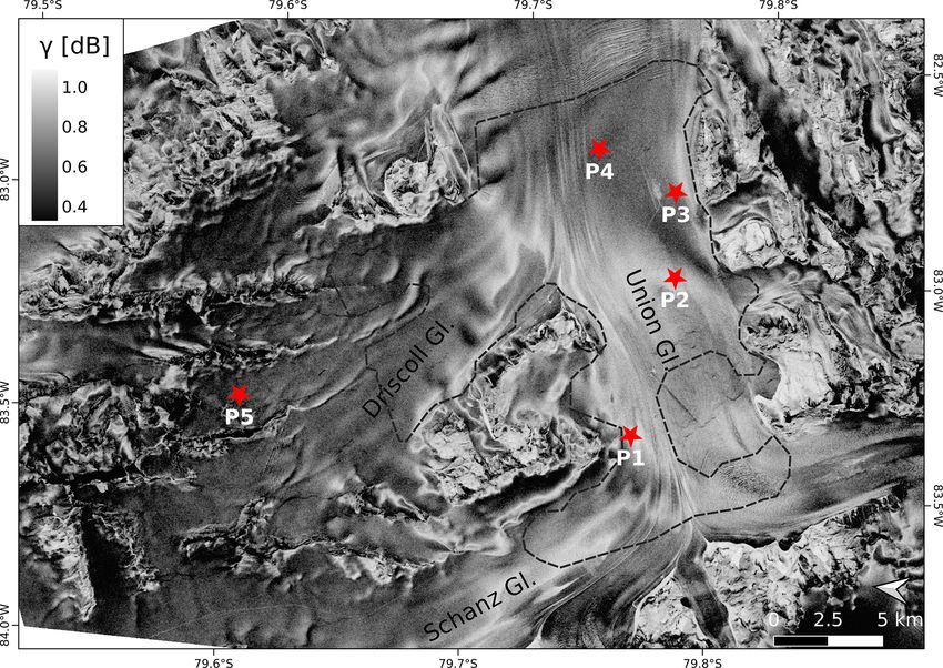
4402                                           H. Rott et al.: Penetration of interferometric radar signals in Antarctic snow

tended homogeneous areas (fixed blocks) located in differ-         2.3   Topographic data from optical satellite sensors
ent sections of the ice sheet. For the areas in between, the
elevation is adjusted by spatial interpolation between these       Topographic data from the ICESat and ICESat-2 missions
blocks, regionally applying bulk values that are not account-      and the Reference Elevation Model of Antarctica (REMA),
ing for different surface types (Rizzoli et al., 2017a).           derived from very-high-resolution optical stereo images
   For producing DEMs from raw bistatic SAR data (Level 0)         (Howat et al., 2019), are available as a reference for esti-
of individual tracks (the so-called Raw DEMs), we used the         mating the elevation bias in the InSAR DEMs. We use the
operational Integrated TanDEM-X Processor (ITP) of the             ICESat and ICESat-2 data primarily for assessing the tempo-
German Aerospace Center (DLR) (Rossi et al., 2012). The            ral stability of surface elevation. The study area is covered by
Raw DEM pixel spacing is 6 m×3 m. Complementary to each            several tracks of the ICESat and ICESat-2 altimeters. Eleva-
Raw DEM, the ITP provides geocoded rasters of the height           tion data were acquired by ICESat during several campaigns
error (the height error map, HEM), the SAR amplitude, the          between April 2003 and October 2009. We use GLAH12
backscattering coefficient and the interferometric coherence       GLAS/ICESat L2 Global Antarctic and Greenland Ice Sheet
as well as a flag mask indicating critical areas. We applied       Altimetry Data (HDF5), Release 34 (Zwally et al., 2014).
11 × 11 pixel estimation windows for computing the coher-          This product provides geolocated and time-tagged surface
ence maps, adding up to about 390 independent samples for          elevation estimates, referenced to the TOPEX/Poseidon el-
single-polarised data at a 40◦ incidence angle and about 110       lipsoid and corrected for atmospheric delays and tides. The
independent samples for dual-polarised data at a 22◦ inci-         laser footprint size is 60 to 70 m, and the distance between
dence angle. According to the Cramér–Rao bound for coher-          the footprint centres is approximately 170 m. The analysis of
ence estimation, the standard deviation for a coherence mag-       repeat-track data allows the detection of the surface eleva-
nitude of 0.5 amounts to 0.03 for the first case and 0.05 for      tion change after correcting for elevation differences caused
the second case. The uncertainty decreases towards higher          by horizontal shifts in individual footprints. A main cause
coherence values (Bamler and Hartl, 1998). The backscatter         for the height error in ICESat footprints is the uncertainty in
intensity images show maps of the normalised radar cross-          beam pointing, causing slope-induced errors (Brenner et al.,
section σ ◦ . For the computation of σ ◦ , effects of topography   2007; Zwally et al., 2011).
are taken into account for antenna pattern removal and for            Regarding ICESat-2, we use ATLAS/ICESat-2 L3A Land
defining the actual size of the local scattering area. The abso-   Ice Height, Version 2, Land Ice Along-Track Height (ATL06)
lute and relative radiometric accuracies for the TerraSAR-X        product from the time span 14 October 2018 to 1 Septem-
strip map data are estimated at 0.6 and 0.3 dB, respectively       ber 2019. This data set provides geolocated land-ice surface
(Breit et al., 2010).                                              heights above the WGS 84 ellipsoid, ITRF2014 reference
   The HEM delivers the height errors for each DEM pixel           frame, and ancillary parameters including error estimates and
caused by random noise. It is given by the standard deviation      quality flags (Smith et al., 2019a). ATL06 heights represent
of the interferometric phase, for which the coherence and the      the mean surface height averaged along 40 m segments of
number of looks are the main factors. The HEM accounts             ground track, 20 m apart, for each of the six beams of the
neither for the absolute height error (offset) with respect to     Advanced Topographic Laser Altimeter System (ATLAS) in-
a particular geodetic reference system nor for penetration-        strument. The land-ice height is defined as estimated surface
related errors. Low-pass filtering is an efficient means for re-   height of the segment centre for each reference point (Smith
ducing the random height error. The HEM for the TDMgl              et al., 2019b).
DEM of the study region shows over flat terrain and gentle            For spatially detailed comparisons of elevation we use the
slopes random height errors ranging from 0.3 to 1.2 m.             REMA DEM tile no. 32-19 with 8 m posting, covering Union
   Specifications of the TDM data used in this study are listed    Glacier (Howat et al., 2019). The dates of the image ac-
in Table 1. The azimuth resolution of the single-polarisation      quisitions for this tile range from January 2014 to Decem-
data is 3.3 m and of the dual-polarised data 6.6 m. The ground     ber 2015. The absolute height is based on vertical registration
range resolution is 3.20 m at θi = 22◦ and 1.86 m at θi = 40◦ .    to CryoSat-2 altimetry data, acquired in SAR interferomet-
We selected scenes with different incidence angles and base-       ric (SARIn) mode. In order to account for the CryoSat sig-
lines in order to check the impact of these parameters on          nal penetration, a uniform value of 0.39 m was added to the
coherence, backscatter intensity and signal penetration. Ac-       CryoSat-2-registered heights over this tile, regardless of the
cording to the HEM maps, the random errors for the Raw             surface type (Howat et al., 2019). This needs to be taken into
DEMs, excluding steep slopes, range from 0.7 to 3.0 m. The         account for using the REMA data as an elevation reference
spatial variations can mainly be attributed to phase noise aris-   because the study area includes bare ground, ice surfaces,
ing from thermal and volume decorrelation. For the estima-         and snow and firn with different structural properties affect-
tion of signal penetration we use averages over multiple pixel     ing radar signal penetration. The vertical error estimates for
windows in order to reduce the uncertainty.                        REMA in the region of interest range from 1.0 to 1.4 m. The
                                                                   error value of each pixel is the standard error from the resid-
                                                                   uals of the registration to altimetry (Howat et al., 2019). The

The Cryosphere, 15, 4399–4419, 2021                                                   https://doi.org/10.5194/tc-15-4399-2021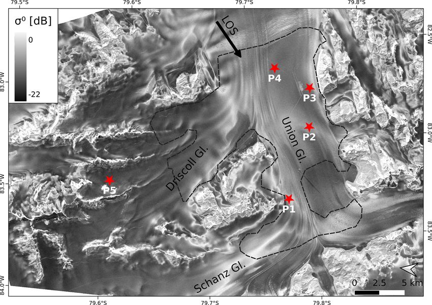
H. Rott et al.: Penetration of interferometric radar signals in Antarctic snow                                                             4403

Table 1. Specifications of TanDEM-X data used for DEM production and generation of backscatter and coherence images. θi is the incidence
angle in the scene centre. Bn is the effective interferometric baseline, Ha is the height of ambiguity, and kzVol is the vertical interferometric
wavenumber in the snow volume assuming a density of 400 kg m−3 . SAR operation mode: bistatic; HH: horizontal transmit and receive
polarisation; VV: vertical transmit and receive polarisation.

      Label      Date             Relative orbit/scene    Look direction    Polarisation    θi [◦ ]    Bn [m]    Ha [m]    kzVol [rad m−1 ]
      T2013A     6 May 2013       105/15                  Left              HH               40.9        107.4    −65.6               0.111
      T2013B     22 May 2013      198/14                  Left              HH               38.6        106.5    −61.2               0.121
      T2014A     9 May 2014       14/7                    Left              HH               37.5        145.8    −42.9               0.173
      T2014B     12 Jun 2014      233/35                  Left              HH               40.8        123.5    −56.6               0.128
      T2016      10 Dec 2016      18/2                    Right             HH and VV        21.6         50.0    −67.3               0.120
      T2018      10 Jan 2018      18/2                    Right             HH and VV        22.1         30.2   −112.0               0.072

Table 2. Mean density of snow–firn for layers of 0.5 m vertical ex-        of snow–firn for layers of 0.5 m vertical extent is specified in
tent of snow pits P1 to P5 on Union Glacier. The snow pit altitude         Table 2. Grain size and hardness show significant differences
refers to the REMA DEM.                                                    between the five measurement sites. The size and shape of
                                                                           the snow grains and the sequence and properties of snow–
                        P1       P2        P3      P4         P5           firn layers are arising from accumulation history, exchange
      Altitude [m]   756.8    690.1    674.1    656.0    1133.3            processes of radiation, turbulent heat and mass at the snow–
                                                                           air interface, and vapour diffusion in the snow volume. Down
      Depth                    Snow density [kg m−3 ]
                                                                           to about 2 m depth the temperature gradient metamorphism
      0 to 0.5 m        443     390      323      366        286           is the dominating process for grain growth, triggered by sea-
      0.5 to 1.0 m      499     422      408      369        372           sonal temperature variations (Alley, 1988; Colbeck, 1983).
      1.0 to 1.5 m      548     471      399      408        371           Average temperature gradients in the top metre of the five
      1.5 to 2.0 m              467      419      472        451           snow pits were on the order of 10 ◦ C m−1 . Differences in
                                                                           the average grain size of the pits can, at least partly, be at-
                                                                           tributed to the snow age following from differences in the
error due to the use of the bulk CryoSat-2-based penetration               surface mass balance (Sect. 2.1). Courville et al. (2007) stud-
correction is not included in this error estimate.                         ied the microstructure of snow and firn in a megadune re-
                                                                           gion in East Antarctica. They show that local differences in
2.4    Snow pit measurements                                               grain size, thermal conductivity and permeability are related
                                                                           to spatial accumulation variability in which already relatively
For the snow pit measurements, made in December 2016, we                   small differences in the net accumulation due to wind redis-
selected sites covered by ICESat footprints that show differ-              tribution cause significant differences in physical snow prop-
ent values of coherence and backscatter intensity in TDM                   erties.
data. Backscatter properties of dry snow and firn are con-                    Snow pit 1 exhibits the largest grains, the highest snow
trolled by snow microstructure, which is also a main factor                density, thin ice layers and several wind crusts. Accumu-
for X-band radar signal penetration. In the study region the               lation data are not available, but from the closeness to the
impact of melt for snow metamorphism is marginal. We de-                   BIA it can be concluded that the mean accumulation rate is
tected evidence for melt events in two of the five snow pits:              well below the accumulation rate near the ALE camp. Due
a thin ice crust at 1.1 m depth of pit 5 and two thin ice crusts           to the high exposure to katabatic winds the stratification does
along with one ice layer of 4 cm thickness in pit 1. The tem-              not allow an identification of annual accumulation layers. In
perature record from March 2010 to February 2014 at the                    some years sublimation and wind erosion may result in neg-
meteorological station near the runway shows a mean annual                 ative mass balance. The higher hardness values compared to
air temperature of −21.1 ◦ C and mean monthly temperatures                 the other sites can be attributed to more frequent exposure
of −8.6 ◦ C for December and −9.3 ◦ C for January. During                  to high wind speeds, the erosion and deposition of blowing
those years a few short events with air temperatures close to              snow, and greater age due to low accumulation. Two thin ice
the melting point were recorded.                                           crusts (5 mm thickness) at 0.49 and 1.25 m depth possibly
   Profiles of snow density, temperature, hardness, grain size             trace back to radiation penetration causing melt below the
and shape are shown in Fig. 2. The pits vary in depth between              frozen surface (Colbeck, 1989). An ice layer of 4 cm thick-
1.6 and 2.3 m. The observed grain size refers to the maximum               ness between 1.38 and 1.42 m depth, with air bubbles of up
axis length of prevailing grains (Fierz et al., 2009). Hardness            to 2 mm size, indicates an intensive melt event.
was estimated by the hand test, ranging from very low (R1)
to very high (R5) for snow and R6 for ice. The mean density

https://doi.org/10.5194/tc-15-4399-2021                                                               The Cryosphere, 15, 4399–4419, 2021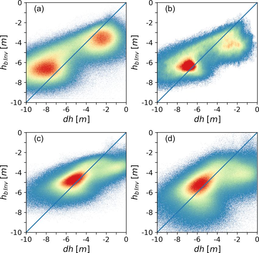
4404                                             H. Rott et al.: Penetration of interferometric radar signals in Antarctic snow

Figure 2. Vertical profiles of snow temperature, density, grain size (GS), grain shape and hand hardness (R) for snow pits P1 to P5 on Union
Glacier, December 2016. The grain size refers to the maximum axis length of the prevailing snow grains.

The Cryosphere, 15, 4399–4419, 2021                                                          https://doi.org/10.5194/tc-15-4399-2021
H. Rott et al.: Penetration of interferometric radar signals in Antarctic snow                                                 4405

   P2 is the snow pit with the highest average snow density        The terms on the right-hand side refer to the interferomet-
next to P1. It is located halfway between the runway and the       ric correlation coefficient related to the signal-to-noise ratio
ALE camp, more exposed to katabatic winds than the camp            (γtherm ), quantisation (γQuant ), azimuth and range ambigui-
so that the average accumulation rate should be lower than at      ties (γAmb ), baseline decorrelation (γRg ), relative shift in the
P3 and P4. The stratigraphy down to 2 m depth shows four           Doppler spectra (γAz ), volumetric decorrelation (γVol ), and
layers of high density with comparatively fine-grained snow,       temporal decorrelation (γtemp ). Temporal decorrelation is not
typical for wind packs, and several thin wind crusts. Softer       relevant for single-pass InSAR data over ground, including
layers with faceted grains show up below wind packs, but a         snow and ice (γtemp = 1.0).
clear assignment to seasonal or annual layers is not possible.        The thermal interferometric correlation component is re-
   The pits P3 and P4, located in the vicinity of the camp,        lated to the signal-to-noise ratio (SNR) of the two SAR im-
show lower mean density and lower variability in density. P4       ages by
is located slightly upstream of stake B10, for which Rivera et                  r
al. (2014) report a specific mass balance bn = 0.17 m w.e. a−1     γtherm = 1/       1 + SNR−1    1 + SNR−1 .                    (2)
                                                                                            1            2
for 2008–2009. Down to the depth of 2.0 m the P4 strat-
ification shows four comparatively thick, hard layers with         For single-pass InSAR the volumetric correlation coefficient
rounding depth hoar below. The total snow mass down to             can be derived from the total coherence by
2.0 m amounts to 0.81 m w.e. Assuming that the transitions
                                                                                     γtot
from hard to soft layers correspond to late summer hori-           γVol =                            .                      (3)
zons and accounting for the lack of 2 months to cover the                 γtherm γQuant γAmb γRg γAz
full 4-year period imply an annual accumulation rate bn =          The phase noise due to γAmb , γQuant and γAz of advanced
0.21 m w.e. a−1 . At P3 the sequence of layers is less distinct.   SAR systems is small. For TDM single-pass InSAR interfer-
This site is located at a cross-wind distance of 300 m from        ograms Krieger et al. (2007) estimate the typical loss of co-
the camp and may be affected by local perturbations of snow        herence for each of the terms γAmb , γQuant and γAz at < 2 %.
drift during summer, when the camp is set up to a full extent.     Baseline decorrelation, γRg , is avoided by applying common
   P5 is located at 1133 m elevation on a flat section of a        bandwidth filtering.
slanting lateral branch of Driscoll Glacier that extends up-          Hoen and Zebker (2000) specify a formulation for the cor-
hill towards the Pioneer Heights, 400 m in altitude above the      relation factor in a uniform volume with exponential extinc-
confluence with Union Glacier. The site is not exposed to          tion in which the interferometric phase is proportional to the
the strong katabatic winds that are blowing along the main         penetration length, dl :
branch of Union Glacier. The grain size is smaller, and the
                                                                                           √
                                                                             s
                                                                                                    2
snow is softer than at the other sites. A melt crust of 3 mm

                                                                                      pπ εdl Bn
thickness was found at 1.14 m depth, most likely related to        γVol = 1/ 1 +
                                                                                        r0 λ tan θi
a short event with comparatively warm temperatures on 17–
                                                                                     √
                                                                             s
                                                                                                     2
18 January 2016. The snow mass above this crust amounts                               π εdl cos θi
to 0.38 m w.e. A thin hard layer at 2.11 m depth with a soft,           = 1/ 1 +                        ,                     (4)
                                                                                            Ha
coarse-grained layer below refers probably to the 2015 late-
summer horizon. The snow mass between the wind crust in            where λ is the radar wavelength, r0 is the slant range dis-
late summer 2015 and the melt crust in January 2016, a pe-         tance, θi is the incidence angle at the air–snow interface, Bn
riod of about 11 months, amounts to 0.41 m w.e. These two          is the effective interferometric baseline, and ε is the dielectric
accumulation estimates indicate for this site about twice the      permittivity; p = 1 is valid for the combination of one mono-
accumulation rate on the main glacier near the ALE camp.           static and one bistatic SAR image forming an interferogram
                                                                   and p = 2 for the combination of two monostatic images. Ha
                                                                   is the height of ambiguity in free space:
3   Interferometric coherence and penetration-related                      λr0 sin θi
    elevation bias                                                 Ha =               .                                          (5)
                                                                             pBn
The procedure for estimating the interferometric elevation         According to the radiative transfer approach the one-way
bias is based on the inversion of the volumetric correlation       power penetration length dl [m], where the intensity of the
factor, which can be derived from total coherence products         signal is attenuated to 1/e of the incident signal, is given by
(γtot ) generated during InSAR processing. The total inter-               1       1
ferometric complex correlation coefficient (coherence) of a        dl =      =         ,                                         (6)
                                                                          ke   ks + ka
random medium is made up of the following contributions
(Krieger et al., 2007):                                            where ka and ks [m−1 ] are the absorption and the scattering
                                                                   coefficients. The one-way power penetration depth, dp , re-
γtot = γtherm · γQuant · γAmb · γRg · γAz · γVol · γtemp .   (1)   ferring to vertical direction, is obtained by accounting for the

https://doi.org/10.5194/tc-15-4399-2021                                                    The Cryosphere, 15, 4399–4419, 2021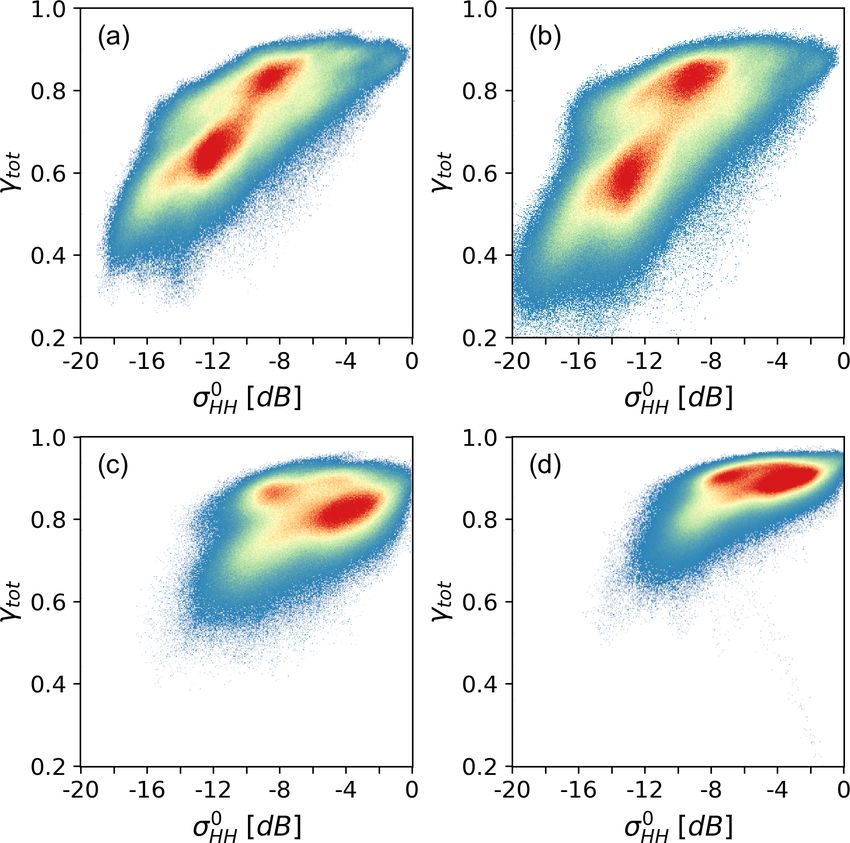
4406                                           H. Rott et al.: Penetration of interferometric radar signals in Antarctic snow

refraction angle θr :                                                 This approach is based on the assumption of a uniform
                                                                   volume with exponential extinction, whereas dry polar firn is
dp = dl cos θr .                                            (7)
                                                                   a density-stratified medium featuring distinct differences in
The vertical interferometric wavenumber, kz [rad m−1 ], re-        scattering and extinction properties between individual lay-
lates the phase of the interferometric correlation to the ge-      ers as well as depth-dependent changes. However, for invert-
ometric configuration of the interferometer, providing phase       ing the observed interferometric coherence in terms of the el-
(ϕ) to height conversion:                                          evation bias the assumption of a simple model is needed for
       ∂ϕ   2π                                                     describing the vertical backscatter and extinction properties.
kz =      =    .                                            (8)    We tested the applicability of the uniform volume approach
       ∂z   Ha
                                                                   for describing the observed backscatter intensity, perform-
The wavenumber in a lossy volume accounts for the change           ing forward computations with a multilayer radiative transfer
in the propagation constant and refraction (Lei at al., 2016),     model (see Appendix A).
yielding the following formulation for the height of ambigu-
ity in the volume:
                                                                   4     Analysis of backscatter signatures, coherence and
         2π                                                              elevation bias
HaVol =       ,                                             (9)
        kzVol
where                                                              In this section we show the spatial pattern of backscatter in-
          √ cos θi                                                 tensity and coherence in the study area and relations of these
kzVol = kz ε        .                                              parameters to the elevation bias inferred from optical sensor
             cos θr                                                data. We start with an account of topographic reference data
For dry snow and ice the absorption, losses are very small         and the procedures applied for vertical co-registration, a crit-
so that the real part of the permittivity can be used (Mätzler,    ical step for estimating the penetration-related elevation bias.
1996). In Table 1 the values for Ha and for kzVol (assuming
a snow density of 400 kg m−3 ) are specified for the TDM           4.1     Topographic reference and vertical co-registration
scenes.
   Dall (2007) shows that the penetration-related elevation        The precise vertical co-registration on surfaces that are not
bias, hb , is approximately equal to the two-way power pen-        subject to radar signal penetration is essential for obtaining
etration depth, dp2 , if the latter is small compared to HaVol .   reliable estimates on the interferometric elevation bias. If the
For large relative penetration depths (dp2 /HaVol ) the eleva-     data to be co-registered are lacking temporal coincidence,
tion bias approaches one-quarter of the ambiguity height.          checks on the temporal stability of the surfaces are needed.
Normalising the coherence phase, 6 γ , by the interferomet-        These topics are addressed below.
ric phase at the volume surface (6 γ = ϕ − ϕsurface ) yields the
                                                                   4.1.1    Notations for elevation differences
following relation, in which the elevation bias is proportional
to 6 γ (Dall, 2007):                                               The apparent glacier surface in an InSAR DEM refers to the
                    6
                   γ |HaVol |                                      position of the scattering phase centre in the snow and firn
hb = 6 γ /kzVol =             .                        (10)        volume. The elevation bias, hb , is the difference between the
                      2π
For a uniform volume a direct relationship between the co-         apparent elevation derived by means of the InSAR method,
herence magnitude and the relative penetration depth can be        hinsar , and the true surface elevation, hs :
defined, from which the phase can be computed (Dall, 2007):        hb = hinsar − hs .                                         (13)
                           q
6 γ = −sgn (HaVol ) arctan             −2
                                |γVol | − 1 .          (11)        For the elevation bias estimate derived from the volumetric
                                                                   coherence by means of Eq. (12) we use the notation hbInv .
As according to this relation the coherence phase is uniquely      For studying the penetration-related elevation bias we co-
defined by the coherence magnitude, the following formula-         register the TDM DEMs on surfaces devoid of penetration
tion can be used for estimating the elevation bias:                with elevation data of optical sensors. On these surfaces the
                       q                                         raw TDM DEMs show vertical offsets up to a few metres
         HaVol                                                     because for these data only a preliminary adjustment for ab-
hb = −          arctan     |γVol |−2 − 1 .               (12)
          2π                                                       solute height is performed with ITP processing. We use the
We apply this equation for estimating the elevation bias from      notation 1h for specifying the elevation difference between
the observed coherence, using the magnitude of the volumet-        optical data and the vertically unregistered TDM DEMs:
ric InSAR correlation factor as input. According to this for-
                                                                   1h = hoptical − hTDM,unreg .                               (14)
mulation the actual InSAR elevation bias becomes progres-
sively smaller than dp2 with increasing relative penetration       Suitable targets for vertical co-registration in the study area
depth.                                                             are the BIA and bare ground on an ice-free slope bordering

The Cryosphere, 15, 4399–4419, 2021                                                     https://doi.org/10.5194/tc-15-4399-2021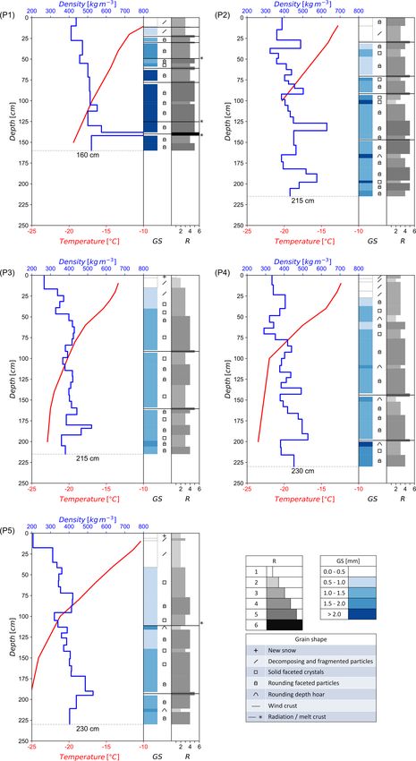
H. Rott et al.: Penetration of interferometric radar signals in Antarctic snow                                              4407

the BIA (“S” in Fig. 1). We use the notation dh for the ele-       near pit 4, where the penetration bias is several metres. The
vation difference between the TDM DEMs and optical ele-            ICESat data set comprises seven closely spaced tracks ac-
vation data, vertically co-registered on surface scattering tar-   quired between 11 April 2003 and 12 February 2008. The
gets:                                                              mean value and standard deviation of the elevation differ-
                                                                   ence between ICESat and the TDMgl DEM are on the central
dh = hTDM,coreg − hoptical .                               (15)    section of the glacier: 1h = 0.09 m, σh = 0.40 m (Table S2).
In the case of temporal coincidence or stable topography, dh       The mean 1h values on individual dates range from −0.03 to
corresponds to the interferometric elevation bias. Though the      0.21 m without any obvious temporal trend, confirming also
time series of ICESat data indicate temporal stability of sur-     the temporal stability of surface elevation. Subtracting the
face elevation in the study area, minor errors due to temporal     TDMgl offset of −6.76 m from the mean 1h value (0.09 m)
changes in elevation cannot be fully excluded.                     yields an elevation bias (dh) of −6.67 m due to signal pene-
                                                                   tration.
4.1.2   Temporal stability of surface elevation
                                                                   4.1.3    Vertical co-registration of the DEMs
Because of the lack of temporal coincidence between the
TDM and optical elevation data, we checked the temporal            We use REMA elevation data as a reference in order to ob-
variability using ICESat time series. The main section of the      tain spatially detailed estimates of the interferometric eleva-
BIA was crossed by ICESat repeat tracks on seven dates be-         tion bias. The mean value and standard deviation of the ele-
tween May 2004 and November 2009 (Fig. 1). The mean                vation difference between ICESat and REMA over the BIA
difference in elevation 1h between the ICESat footprints in        are 1h = −0.33 m, σ1h = 0.38 m (Table S1). This value dif-
the BIA and the corresponding TDMgl cells (mean values of          fers by 6 cm from the bulk penetration correction (−0.39 m)
5 × 5 pixels) is −6.76 m. The standard deviation for the 126       applied to the CryoSat-2 elevation data that are used as an
samples of the time series is 0.43 m (Table S1 in the Sup-         absolute height reference for the REMA DEM (Howat et al.,
plement). The mean 1h values on the different dates range          2019). This correction introduces a bias over bare ice where
from −6.61 to −6.86 m without any distinct temporal trend,         the actual CryoSat-2 signal refers to surface reflection. On
indicating high temporal stability. The stability of surface el-   the ice-free slope the elevation differences in REMA ver-
evation in the BIA is also confirmed by the GPS time se-           sus ICESat, ICESat-2 and TDMgl elevation data show high
ries of Rivera et al. (2014). The 1h value of −6.76 m can          standard deviations. Therefore we use the BIA as a reference
be mainly attributed to the bulk penetration correction that       site for vertical co-registration between the TDM DEMs and
is applied for TDMgl DEM products over Antarctica. The             REMA.
ICESat-2 data set of the BIA includes eight tracks with al-           For cross-comparing the TDM and REMA elevation data
together 345 spots, extending along the eastern and western        we outlined an area of 5 km2 extent in the central section
margins of the BIA, which are occasionally covered by snow.        of the BIA that is crossed by the ICESat tracks, avoiding
The mean elevation difference and standard deviation are 1h        BIA sections that are occasionally covered by snow. The
(ICESat-2-TDMgl) = −6.99 m, σ1h = 0.38 m.                          mean elevation difference 1h between REMA and TDMgl
   In order to check the validity of the assumption that the       is −6.37 m; the standard deviation at 8 m × 8 m pixel size
BIA signal arises from surface scattering, we derived optical      is 0.62 m. We use the value of −6.37 m for vertical co-
versus SAR elevation differences also on the ice-free slope        registration of the TDMgl DEM. The same polygon is used
in the vicinity of the BIA. This slope has a mean inclination      for vertical co-registration of the other TDM DEMs, which
of about 16◦ and contains sections of varying steepness. On        as unregistered DEMs show vertical shifts vs. REMA of −2
slopes, horizontal shifts between pixels to be co-registered       to −3 m.
cause slope-dependent elevation biases, in particular for data
from sensors with different observation geometries and spa-        4.2     Spatial pattern of backscatter signals and
tial resolution (Nuth and Kääb, 2011). Therefore we use data               coherence
from moderately inclined slope sections for quantifying the
vertical offsets. In order to avoid steep slope sections we ex-    Figure 3 shows an image of the backscatter cross-section
cluded all cells of 5×5 TDM pixels with a standard deviation       (σ ◦ ) and Fig. 4 an image of the magnitude of the com-
of elevation larger than 5 m. Under this constraint only 21        plex interferometric correlation coefficient (the total nor-
ICESat pixels of the whole time series qualify for the com-        malised coherence), derived from TDM data of 6 May 2013
parison on the slope, yielding a mean 1h of −6.91 m and            (scene T2013A). For detailed analysis of radar signatures
σ1h of 0.84 m. The difference in the mean 1h values be-            and the elevation bias of snow and firn, we focus on an area
tween the slope and the BIA is below the measurement un-           stretching out over sections of the main glacier and Driscoll
certainty.                                                         Glacier that are completely covered by any of the available
   Another ICESat time series for checking the temporal be-        TDM scenes (the area of interest, AoI). Slopes larger than 5◦
haviour of surface elevation extends across the main glacier       inclination and blue ice areas are excluded. Major blue ice ar-

https://doi.org/10.5194/tc-15-4399-2021                                                  The Cryosphere, 15, 4399–4419, 2021
4408 H. Rott et al.: Penetration of interferometric radar signals in Antarctic snow Figure 3. Section of TDM backscatter image, HH polarisation, 6 May 2013. LOS (line of sight) indicates the radar look direction. Incidence angle in the scene centre (θi ): 40.9◦ . The outline encloses the snow and firn area of interest (AoI) for analysis of radar signatures and the elevation bias. Figure 4. Image of total normalised coherence, γtot , from the TDM interferogram of 6 May 2013. eas are located in the vicinity of the landing strip, on Schanz The spatial pattern of backscatter intensity in the firn areas Glacier, and at the confluence of Driscoll and Union glaciers. of the main glacier and its tributaries primarily reflects differ- The slope constraint reduces impacts of errors in optical and ences in volume-scattering properties and to some extent also SAR DEM co-registration and effects of foreslopes and lay- the pattern of the elevation bias (Sect. 5). Low σ ◦ values in over that vary with the observation geometry of the different the AoI refer to areas of comparatively fine-grained snow and SAR tracks. firn in the top layers, whereas high values are an indication of The Cryosphere, 15, 4399–4419, 2021 https://doi.org/10.5194/tc-15-4399-2021
H. Rott et al.: Penetration of interferometric radar signals in Antarctic snow                                                     4409

                                                                    Figure 6. Scatterplot of the backscatter coefficient σ ◦ HH (dB)
                                                                    vs. the total normalised coherence, γtot , in the AoI. (a) 6 May 2013
Figure 5. Difference in the HH-polarised backscatter coefficients   (θi = 40.9◦ ), (b) 22 May 2013 (θi = 38.6◦ ), (c) 10 December 2016
between the TDM images from 6 May 2013 (θi = 40.9◦ ) and 10 De-     (θi = 21.6◦ ), (d) 10 January 2018 (θi = 21.1◦ ). The colour repre-
cember 2016 (θi = 21.6◦ ), σ ◦ HH 2013 minus σ ◦ HH 2016 (dB).      sents the 2D data density increasing from blue to red. The reduced
                                                                    range of coherence in (d) compared to (c) can be attributed to the
                                                                    shorter effective baseline.

large scattering elements. The blue ice areas have a compara-          The coherence image of 6 May 2013 (Fig. 4) shows the
tively smooth surface, accounting for low σ ◦ at an incidence       lowest coherence on glacier sections with the largest eleva-
angle of 40◦ . The lowest σ ◦ values show up on tributary           tion bias located on Driscoll Glacier and near the ALE camp
glaciers away from the main passage of the katabatic wind.          (γtot = 0.50 to 0.65). In the T2013 and T2014 (T2013/14)
Low σ ◦ is also evident at locations of increased accumulation      TDM images, the coherence of the BIA is also comparatively
rates in the vicinity of the camp. At lower incidence angles        low (mean γtot = 0.79) because of thermal decorrelation due
σ ◦ is higher throughout, and the overall dynamic range of σ ◦      to the low SNR. In the low-accumulation areas surrounding
is reduced, as is evident in Fig. S1, which shows backscatter       the BIA the σ ◦ values range from −5 to −8 dB, and the mag-
and coherence images of 10 December 2016.                           nitude of γtot ranges from 0.85 to 0.90. The incidence angle
   The incidence angle dependence of σ ◦ in the vicinity of         also has an impact on the relation between coherence and
the BIA and in crevasse zones is rather small (Fig. 5). In          σ ◦ . This is evident by comparing scatterplots of scenes with
these areas the differences in σ ◦ between the scenes T2013A        different incidence angles (Fig. 6). The two scenes with in-
(θi = 40.9◦ ) and T2016H (θi = 21.6◦ ) amount to about 3 dB,        cidence angles of 40.9 and 38.6◦ , respectively, show an ap-
and σ ◦ is high in both scenes. This is an indication of large      proximately linear relation between coherence and σ ◦ , with
scattering elements relative to the wavelength. Multiple scat-      two cluster centres corresponding to the surroundings of the
tering between individual layers and scattering at rough inter-     BIA and to areas with higher accumulation rates, respec-
nal interfaces may also play a role. In the areas with higher       tively. The scenes with a 22◦ incidence angle (T2016/18)
accumulation rates the incidence angle dependence is larger,        show reduced dynamic range of coherence and σ ◦ . The vol-
reaching values up to 8 dB in the vicinity of pit 4. Large          umetric normalised coherence, derived from the observed to-
angular backscatter differences in the stratified snow–firn         tal coherence according to Eq. (3), shows the expected trend,
medium can be explained by increased backscatter contri-            i.e. decrease in γVol with increasing baseline (decreasing Ha )
butions of internal interfaces towards near-nadir angles. The       at a given incidence angle (Table 3). The lowest mean co-
pronounced σ ◦ increase towards low incidence angles in the         herence value over the AoI is observed for scene T2014A
BIA (−13.3 dB in scene T2013A, −5.9 dB in T2016H) is                (|Ha | = 42.9 m, γVol = 0.656).
characteristic for backscattering of slightly rough surfaces
(Fung, 1994).

https://doi.org/10.5194/tc-15-4399-2021                                                    The Cryosphere, 15, 4399–4419, 2021
4410 H. Rott et al.: Penetration of interferometric radar signals in Antarctic snow
Figure 8. Elevation difference (dh) TDM DEM − REMA versus the
computed elevation bias, derived from the volumetric coherence for
the snow pit sites P1 to P5. The dashed line is the linear regression
line.
to dh, and the scene T2018 with the shortest |Ha | shows the
lowest sensitivity.
The incidence angle also has an effect on the elevation
bias. For example, the two scenes with almost the same
Figure 7. Relations between the elevation difference (dh) height of ambiguity show different mean dh values of the
TDM − REMA and volumetric coherence (a, b) as well as between snow pit sites (Table S4) – T2013A: |Ha | = 65.6 m, hdhi =
the elevation difference and the backscatter coefficient (c, d) for the 5.93 m; T2016: |Ha | = 67.3 m, hdhi = 4.35 m. The same be-
snow pit sites P1 to P5. The framed points refer to P5. Incidence haviour is evident for the mean dh of the AoI (Table 3):
angle in the swath centre: (a, c) θi = 37.5 to 40.9◦ , (b, d) θi = 21.6 hdhi = 5.97 m for T2013A and hdhi = 4.38 m for T2016.
and 22.1◦ . Regarding polarisation, there are no significant differ-
ences between HH- and VV-polarised data for γVol and dh.
Whereas the snow pit sites show slightly larger |dh| at HH
polarisation, over the AoI this is the case at VV polarisation.
4.3 Backscatter signatures, coherence and elevation The differences in σ ◦ and coherence between HH and VV
bias at the snow pit sites polarisation are also small. The average σ ◦ HH of the snow
pit sites is 0.28 dB lower than σ ◦ VV .
The backscatter coefficients, the magnitude of the total and The plots of dh vs. σ ◦ at the snow pits in Fig. 7 indicate
volumetric correlation coefficients and the elevation bias for for the T2013/14 scenes an approximately linear relation for
cells with 90 m diameter centred at the snow pit sites are the sites P1 to P4, but the data of P5 (hσ ◦ i = −16.3 dB) are
listed in Tables S3 and S4. The speckle-related uncertainty shifted by a few decibels. The reduced σ ◦ of P5 can be at-
(standard deviation) of σ ◦ for the 90 m cells is 0.13 dB tributed to the smaller grain size and a smoother vertical den-
for the single-polarised data at θi = 40◦ (T2013/14 scenes) sity profile. The T2016/18 data do not show any obvious re-
and 0.26 dB for the HH- and VV-polarised data at θi = 22◦ lation between dh and σ ◦ . P4 (σ ◦ HH −2.8 dB) and P5 (σ ◦
(T2016/18 scenes). The γ values are based on the coher- HH −11.0 dB) have a similar elevation bias. The same be-
ence pixels whose centre coordinates fit within the corre- haviour as for P4, comparatively deep penetration and high
sponding 90 m cell. Pit 5 is not covered by the scenes T2016 σ ◦ in the T2016/18 data, is evident for an extended area in its
(10 December 2016) and T2018 (10 January 2018). We de- surroundings which shows high backscatter in the T2016/18
rived the data for pit 5 from two scenes of adjoining tracks data (mean σ ◦ = −3 dB) and a comparatively large elevation
with similar height of ambiguity and incidence angle: 7 Jan- bias (mean dh = −5 m). The high σ ◦ at near-nadir angles is
uary 2017 (θi = 24.6◦ , Ha = −70.0 m) and 16 January 2018 an indication of increased backscatter at internal interfaces,
(θi = 24.7◦ , Ha = −106.0 m). but it is not clear why this has less impact on volume decor-
Figure 7 shows plots of the volumetric coherence and the relation.
backscatter coefficient versus the elevation difference dh be-
tween the TDM DEMs and the REMA at the snow pit sites.
In order to point out effects of the incidence angle, the data 5 Estimation of the interferometric elevation bias
derived from the T2013/14 and from the T2016/18 scenes are
displayed separately. There is a clear trend of decrease in γVol Building on the signature analysis reported in Sect. 4, we
with increasing magnitude of dh. The scene T2014A with the focus on the use of the volumetric coherence for estimating
largest |Ha | shows the highest sensitivity of γVol with respect the interferometric elevation bias by inverting γVol according
The Cryosphere, 15, 4399–4419, 2021 https://doi.org/10.5194/tc-15-4399-2021H. Rott et al.: Penetration of interferometric radar signals in Antarctic snow 4411
Table 3. Mean values over the AoI for the elevation difference TDM − REMA (dh), the TDM elevation bias by inversion of volumetric
coherence (hbInv ), the difference between dh and hbInv , the volumetric coherence (γVol ), and the backscatter coefficient (σ ◦ ). R 2 is the
coefficient of determination for linear correlation between dh and hbInv ; RMSD is the root mean square difference between dh and hbInv .
T2013A T2013B T2014A T2014B T2016H T2016V T2018H T2018V
dh [m] −5.97 −5.63 −5.49 −5.10 −4.28 −4.48 −4.78 −4.82
hbInv [m] −5.80 −5.43 −4.85 −4.78 −4.39 −4.40 −5.17 −5.19
dh − hbInv [m] −0.17 −0.20 −0.64 −0.32 0.11 −0.08 0.39 0.37
γVol 0.791 0.778 0.656 0.808 0.864 0.858 0.927 0.926
σ ◦ [dB] −9.37 −9.95 −8.21 −9.12 −5.21 −5.36 −4.49 −4.71
R2 0.57 0.59 0.47 0.49 0.41 0.27
RMSD [m] 1.88 1.84 2.03 1.56 1.43 1.79
to Eq. (12). For computing the vertical wavenumber in the be larger in scenes with smaller off-nadir angles in the case
volume and the refraction angle, we assume a snow density of the same value of Ha .
of 400 kg m−3 , resulting in ε 0 = 1.763 (Mätzler, 1996). Fig- The AoI mean values of dh and hbInv show minor differ-
ure 8 shows plots of the computed elevation bias, hbInv , at the ences: −0.33 m for T2013/14 and 0.20 m for T2016/18. The
snow pit sites derived from γVol vs. the elevation difference spatial patterns of dh and hbInv are similar, but the mean
dh between the InSAR DEMs and the REMA. The T2013/14 slope of the 2D distribution deviates from the 1 : 1 corre-
data show a highly significant linear relation between dh and spondence (Fig. 11). The magnitude of the computed eleva-
hbInv , with a coefficient of determination R 2 = 0.86. The root tion bias is overestimated over the areas with coarse-grained
mean square difference (RMSD) is 0.74 m, attributed to er- firn and small penetration depth in the surroundings of the
rors in the computed hbInv and the DEM difference product. BIA and underestimated in areas of higher accumulation rate.
The T2016/18 data (mean of HH and VV polarisation) show These depth-dependent deviations can, at least partly, be at-
a linear relation with R 2 = 0.59 and RMSD = 0.84 m. tributed to the simplified assumption of the uniform volume
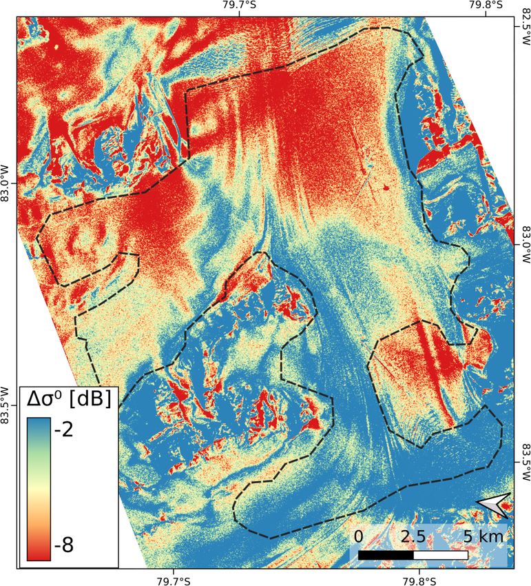
Maps of dh and the computed TDM elevation bias are approach.
shown in Fig. 9 for scene T2013B and in Fig. 10 for scene
T2016. These two scenes have almost the same vertical
wavenumber but different incidence angles. The differences 6 Discussion
between HH- and VV-polarised data of the T2016 and T2018
scene, respectively, are insignificant. We use the mean value A critical issue for inverting interferometric coherence in
of the HH- and VV-based DEMs of the single dates for the terms of the InSAR elevation bias is the description of the
comparison in order to reduce the impact of random phase vertical backscattering profile in the snow volume. A sim-
noise. In Table 3 mean numbers over the AoI are specified ple model is required, in particular if only single-channel
for dh, hbInv , γVol , the coefficient of determination (R 2 ) for backscatter data are available. We apply the model of Dall
linear correlation between dh and hbInv , and the RMSD. The (2007), in which the vertical backscatter function is defined
numbers for R 2 and RMSD refer to the maps resampled to by the extinction coefficient of a uniform random volume ac-
8 m grid size, low-pass filtered over 7 × 7 pixels windows us- counting for the combined effect of absorption and scatter-
ing a Gaussian function. The dh value of the TDMgl DEM ing. In order to check the suitability of this model for de-
(dh = 5.61 m) differs only by 0.06 m from the mean dh of the scribing the backscattering profile of layered polar firn, we
T2013/14 data. The TDMgl DEM is based on several TDM performed backscatter simulations for the snow pit sites with
scenes acquired in 2013 and 2014. The dh map for TDMgl a multilayer radiative transfer model (Appendix A).
vs. REMA shows a similar spatial pattern as dh of the indi- The computed total σ ◦ values at θi = 40◦ are matching the
vidual DEMs (Fig. S2). observed total backscatter intensities of the T2013/14 scenes
As for the snow pit sites, the mean values over the AoI for snow pit sites 2 to 5. The simulated vertical backscatter
show distinct differences in dh, hbInv and γVol between the profiles and the exponential profiles of the uniform volume
data sets with different incidence angles. The magnitudes of approach show close agreement for sites 2 to 4. The varia-
the elevation bias of the T2013/14 data (mean dh = −5.55 m, tions between individual layers, tracing back to accumulation
hbInv = −5.22 m) are larger than the corresponding values of and wind erosion events as well as to seasonal effects, are
the T2016/18 data set (dh = −4.59 m, hbInv = −4.79 m). As suppressed in the vertical profile of the cumulative backscat-
for the snow pit sites, this is opposite to the expectation for ter contributions. At sites 2 to 4 the uniform volume approach
a uniform isotropic scattering medium for which |hb | should shows minor overestimation of the backscatter contributions
from the top snow layers due to the assumption of a con-
stant scattering coefficient, whereas the actual grain size in
https://doi.org/10.5194/tc-15-4399-2021 The Cryosphere, 15, 4399–4419, 2021You can also read