On the diurnal, weekly, and seasonal cycles and annual trends in atmospheric CO2 at Mount Zugspitze, Germany, during 1981-2016
←
→
Page content transcription
If your browser does not render page correctly, please read the page content below
Atmos. Chem. Phys., 19, 999–1012, 2019
https://doi.org/10.5194/acp-19-999-2019
© Author(s) 2019. This work is distributed under
the Creative Commons Attribution 4.0 License.

On the diurnal, weekly, and seasonal cycles and annual trends in
atmospheric CO2 at Mount Zugspitze, Germany, during 1981–2016
Ye Yuan1 , Ludwig Ries2 , Hannes Petermeier3 , Thomas Trickl4 , Michael Leuchner1,5 , Cédric Couret2 , Ralf Sohmer2 ,
Frank Meinhardt6 , and Annette Menzel1,7
1 Department    of Ecology and Ecosystem Management, Technical University of Munich (TUM), Freising, Germany
2 German    Environment Agency (UBA), Zugspitze, Germany
3 Department of Mathematics, Technical University of Munich (TUM), Garching, Germany
4 Institute of Meteorology and Climate Research, Atmospheric Environmental Research (IMK-IFU),

Karlsruhe Institute of Technology (KIT), Garmisch-Partenkirchen, Germany
5 Springer Nature B.V., Dordrecht, the Netherlands
6 German Environment Agency (UBA), Schauinsland, Germany
7 Institute for Advanced Study, Technical University of Munich (TUM), Garching, Germany

Correspondence: Ye Yuan (yuan@wzw.tum.de)

Received: 14 August 2018 – Discussion started: 30 August 2018
Revised: 19 December 2018 – Accepted: 10 January 2019 – Published: 25 January 2019

Abstract. A continuous, 36-year measurement composite             Schauinsland (15.9 ± 1.0 ppm), but following a similar sea-
of atmospheric carbon dioxide (CO2 ) at three measurement         sonal pattern.
locations on Mount Zugspitze, Germany, was studied. For
a comprehensive site characterization of Mount Zugspitze,
analyses of CO2 weekly periodicity and diurnal cycle were
performed to provide evidence for local sources and sinks,        1   Introduction
showing clear weekday to weekend differences, with domi-
nantly higher CO2 levels during the daytime on weekdays. A        Long-term records of atmospheric carbon dioxide (CO2 ) im-
case study of atmospheric trace gases (CO and NO) and the         prove our understanding of the global carbon cycle, as well
passenger numbers to the summit indicate that CO2 sources         as long- and short-term changes, especially at remote back-
close by did not result from tourist activities but instead ob-   ground locations. The longest continuous measurements of
viously from anthropogenic pollution in the near vicinity.        atmospheric CO2 started in 1958 at Mauna Loa, Hawaii, ini-
Such analysis of local effects is an indispensable require-       tiated by investigators of the Scripps Institution of Oceanog-
ment for selecting representative data at orographic com-         raphy (Pales and Keeling, 1965). The measurements were
plex measurement sites. The CO2 trend and seasonality were        performed on the north slope of the Mauna Loa volcano at
then analyzed by background data selection and decompo-           an elevation of 3397 m above sea level (a.s.l.), thus at long
sition of the long-term time series into trend and seasonal       distances from CO2 sources and sinks. Later, additional mea-
components. The mean CO2 annual growth rate over the 36-          surement sites were established for background studies of
year period at Zugspitze is 1.8 ± 0.4 ppm yr−1 , which is in      global atmospheric CO2 , such as the South Pole (Keeling
good agreement with Mauna Loa station and global means.           et al., 1976), Cape Grim, Australia (Beardsmore and Pear-
The peak-to-trough amplitude of the mean CO2 seasonal cy-         man, 1987), Mace Head, Ireland (Bousquet et al., 1996), and
cle is 12.4 ± 0.6 ppm at Mount Zugspitze (after data selec-       Baring Head, New Zealand (Stephens et al., 2013). Along
tion: 10.5 ± 0.5 ppm), which is much lower than at nearby         with sites located in Antarctica or along coastal/island re-
measurement sites at Mount Wank (15.9 ± 1.5 ppm) and              gions, continental mountain stations offer excellent options
                                                                  to observe background atmospheric levels due to high eleva-
                                                                  tions that are less affected by local influences, for example,

Published by Copernicus Publications on behalf of the European Geosciences Union.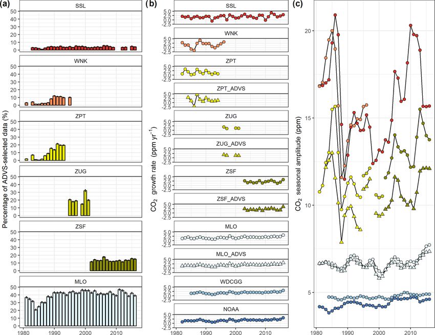
1000                  Y. Yuan et al.: Weekly, seasonal cycles and annual trends in atmospheric CO2 at Mount Zugspitze

Mount Waliguan, China (Zhang et al., 2013), Mount Cimone,         tain. In addition, CO2 measurements were taken at the nearby
Italy (Ciattaglia, 1983), Jungfraujoch, Switzerland, and Puy      lower mountain station, Wank Peak (WNK), but for a shorter
de Dôme, France (Sturm et al., 2005).                             time period. Short-term variations of weekly CO2 periodici-
   Although mountainous sites experience less impact from         ties and diurnal cycles were evaluated for Mount Zugspitze.
local pollution and represent an improved approach to back-       In addition, a case study combining atmospheric CO and NO
ground conditions compared with stations at lower eleva-          measurements and records of passenger numbers was used
tions, we cannot fully dismiss the influence of local to re-      to examine weekday–weekend influences. Then the results
gional emissions. This influence largely depends on air-          for the CO2 annual growth rates and seasonal amplitudes
mass transport and mixing within the moving boundary layer        were studied separately via seasonal-trend decomposition
height. Lidar measurements show that air from the bound-          and compared with CO2 data for the comparable time pe-
ary layer is orographically lifted to approximately 1–1.5 km      riod (1981–2016) at the Global Atmospheric Watch (GAW)
above typical summit heights during daytime in the warm           regional observatory Schauinsland, Germany (SSL), and the
season (Carnuth and Trickl, 2000; Carnuth et al., 2002).          GAW global observatory Mauna Loa, Hawaii (MLO), as well
A 14-year record of atmospheric CO2 at Mount Waliguan             as the global CO2 means calculated by the NOAA/ESRL and
(3816 m a.s.l.), China, reveals significant diurnal cycles and    the World Data Centre for Greenhouse Gases (WDCGG).
depleted CO2 levels during summer that are mainly driven
by biological and local influences from adjacent regions,
although the magnitude and contribution of these influ-           2     Experimental methods and data
ences are smaller than those at other continental or urban
                                                                  2.1    Measurement locations
sites (Zhang et al., 2013). At the Mt. Bachelor Observatory
(2763 m a.s.l.), USA, atmospheric CO2 variations were stud-       Mount Zugspitze is located approximately 90 km southwest
ied in the free troposphere and boundary layer separately,        of Munich, Germany. The nearest major town is Garmisch-
where wildfire emissions were observed to drive CO2 en-           Partenkirchen (GAP; 708 m a.s.l.). Measurements of CO2
hancement at times (McClure et al., 2016). However, it still      were first performed between 1981 and 1997 at a southward-
remains unclear to exactly what extent elevated mountain          facing balcony in a pedestrian tunnel (ZPT; 47◦ 250 N,
sites are influenced by local activities and how to character-    10◦ 590 E; 2710 m a.s.l.) situated about 250 m below the sum-
ize better local sources and sinks at such stations. It is dif-   mit of Mount Zugspitze, which joined the ancient summit
ficult to make quantitative conclusions on the anthropogenic      station of the first Austrian cable car to the Schneefernerhaus
and biogenic contributions to these measurements (Le Quéré        (Reiter et al., 1986). The Schneefernerhaus was a hotel un-
et al., 2009). Analyzing weekly periodicity may be a poten-       til 1992 when it was rebuilt into an environmental research
tial indicator since periodicity represents anthropogenic ac-     station. From 1995 until 2001, a new set of measurements
tivity patterns during 1 week (7 days) without the influence      were made at a sheltered laboratory on the terrace of the
of natural causes (Cerveny and Coakley, 2002). From the           summit (ZUG; 47◦ 250 N, 10◦ 590 E; 2962 m a.s.l.). These two
perspective of modeling and satellite observational systems,      measurement periods were performed by the Fraunhofer In-
studies have shown that the weekly variability has implica-       stitute for Atmospheric Environment Research (IMK-IFU),
tions on the quantification and verification of anthropogenic     and, since 1995 these measurements have been carried out
CO2 emissions, as well as diurnal variability (e.g., Nassar et    on behalf of the German Environmental Agency (UBA).
al., 2013; Liu et al., 2017). Regarding in situ measurements,     Since 2001, to continue contributing to the GAW program,
results from Ueyama and Ando (2016) clearly indicate the          CO2 measurements have been performed at the Environ-
presence of elevated weekday CO2 emissions compared with          mental Research Station Schneefernerhaus (ZSF; 47◦ 250 N,
weekend and/or holiday CO2 emissions at two urban sites in        10◦ 590 E; 2656 m a.s.l.). Approximately 100 m below the
Sakai, Japan. Cerveny and Coakley (2002) detected signifi-        Schneefernerhaus, the glacier plateau Zugspitzplatt can be
cantly lower CO2 concentrations on weekends than on week-         reached from the valley via cable cars or cogwheel trains.
days at Mauna Loa, which was assumed to result from an-           The Zugspitzplatt descends eastward via a moderate to steep
thropogenic emissions from Hawaii and nearby sources.             slope across the Knorrhütte towards the Reintalangerhütte as
   In this study, we present a composite 36-year record           shown in Fig. 1 (Gantner et al., 2003).
of atmospheric CO2 measurements (1981–2016) at Mount
Zugspitze, Germany (2962 m a.s.l.). The objective of this         2.2    Instrumental setup and data processing
study is to achieve an improved measurement site characteri-
zation with respect to historical CO2 data in terms of diurnal    CO2 mole fractions were processed separately because of
and weekly cycles, and to produce a consistent overall anal-      different measurement locations and time periods at Mount
ysis of CO2 trend and seasonality. The CO2 measurements           Zugspitze as described above. Information on the first time
were performed at three locations on Mount Zugspitze: at          period (ZPT) was collected based on personal communica-
a pedestrian tunnel (ZPT), at the summit (ZUG), and at the        tion with corresponding staff, logbooks, and literature re-
Schneefernerhaus (ZSF) on the southern face of the moun-          search (Reiter et al., 1986). The CO2 measurement at ZPT

Atmos. Chem. Phys., 19, 999–1012, 2019                                              www.atmos-chem-phys.net/19/999/2019/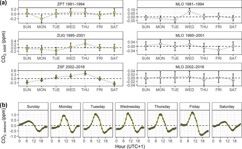
Y. Yuan et al.: Weekly, seasonal cycles and annual trends in atmospheric CO2 at Mount Zugspitze                              1001

Figure 1. (a) Map showing the study area (GAP – Garmisch-Partenkirchen; WNK – Mount Wank; ZPT – pedestrian tunnel at Mount
Zugspitze; ZUG – Zugspitze summit; ZSF – Zugspitze Schneefernerhaus). (b) A photograph showing the locations (ZPT, ZSF, and ZUG) on
Mount Zugspitze at which atmospheric CO2 measurements were performed.

was continuously performed with different instrument mod-           above the pavement of the research terrace on the fifth
els used consecutively (i.e., the URAS-2, 2T, and 3G) em-           floor at an altitude of 2670 m a.s.l. Measurements of CO2 at
ploying the nondispersive infrared (NDIR) technique. The            Schneefernerhaus continued thereafter until the present with
measured values were corrected by simultaneously measured           a modified HP 6890 using a gas chromatograph (GC), with
air pressure with a hermetically sealed nitrogen-filled gas cu-     an intermediate upgrade in 2008 (Bader, 2001; Hammer et
vette due to no flowing reference gas being used. Two com-          al., 2008; Müller, 2009). In 2012 and 2013, because of an in-
mercially available working standards (310 and 380 ppm of           strumental failure of the GC, CO2 data were recorded with a
CO2 in N2 ) were used for calibration every day at different        cavity ring-down spectrometer (CRDS; Picarro EnviroSense
times. The CO2 concentration in this gas bottle was com-            3000i) connected to the same air inlet, which had been in-
pared in short intervals with a reference standard provided         stalled in parallel since 2011. The GC calibrations were car-
by UBA which was adjusted to the Keeling standard refer-            ried out at 15 min intervals using working standards (near-
ence scale.                                                         ambient), which had been calibrated with station standards
   At ZUG the sampling line consisted of a stainless steel          from the GAW Central Calibration Laboratory (CCL) oper-
tube with an inner core of borosilicate glass and a cylindri-       ated by the NOAA/ESRL Global Monitoring Division. The
cal stainless steel top cup to prevent intake of precipitation.     GC data acquisition system (see Supplement Fig. S1) pro-
The inlet was mounted on a small mast (approximately 4 m            duced a calibration value every 15 min and two values from
high) on the top of the laboratory building, which is situ-         the sampled air based on one chromatogram every 5 min.
ated on the Zugspitze summit platform (see Fig. 1b). Inside         For continuous quality assurance the GC was checked daily
the laboratory a turbine with a fast real-time fine control en-     for flows, retention times, gas pressures, and the structure of
sured a constant sample inflow of 500 L min−1 of in situ air.       chromatograms. Calibration factors and metadata were used
The borosilicate glass tube (about 10 cm diameter) contin-          to convert raw data into the final data product. Invalid and
ued inside the laboratory, providing a number of outlets from       unrepresentative data due to local influences were flagged
which the instruments could get the sample air for their own        according to a logged list of local pollution from working ac-
analyses. The measurement and calibration were performed            tivities in the research station. The measurement quality was
with a URAS-3G device and an Ansyco mixing box. The                 controlled by comparison with simultaneous measurements
mixing controller allowed automatic switching for up to four        of identical gas (CRDS) or with measurements of other trace
calibration gases and sampling air by a self-written calibra-       substances and meteorological data, and additional support
tion routine using Testpoint software. The linear two-point         from station logbooks and checklists. The data were flagged
calibration enveloping the actual ambient values with low           according to quality control results. In principle, the acqui-
and high CO2 concentrations was taken every 25th hour. Ev-          sition system stores all measured data (flagged or not) and
ery 6 months the working standards were checked and read-           never discards them. Drifts in the working standards were
justed, when required, according to the standard reference          controlled by a second target (measured approximately 25
scale using intercomparison measurements with the station           times per day) and a regular 2-month intercomparison be-
standards.                                                          tween the working standard and NOAA station standards,
   At ZSF the same construction principle was applied for at-       performing corrections as needed. Calibration for CRDS was
mospheric sampling. There, the mast height is about 2.5 m           performed automatically, with three different concentrations

www.atmos-chem-phys.net/19/999/2019/                                                  Atmos. Chem. Phys., 19, 999–1012, 2019
1002 Y. Yuan et al.: Weekly, seasonal cycles and annual trends in atmospheric CO2 at Mount Zugspitze
every 12 h. Until 2013 the calibrations were performed au- centrations at WNK by calculating the CO2 differences be-
tomatically every 24 h with one concentration, very close to tween ZPT and WNK. A detailed description on the offset
the ambient value. Every 2 months the concentrations were adjustment of CGC with potential errors is given in the Sup-
rechecked according to the station reference standards. plement. Two similar CGCs by Manning and Pohl (1986) at
Additional atmospheric CO2 measurements through- Baring Head, New Zealand, and Cundari et al. (1990) at Mt.
out the GAP area were performed between 1978 and Cimone, Italy, were comparable in magnitude to our offset
1996 at Mount Wank summit (WNK; 47◦ 310 N, 11◦ 090 E; adjustment.
1780 m a.s.l.) using a URAS-2T instrument. Wank Observa- On the other hand, there were 9 consecutive months, from
tory is located in an alpine grassland just above the tree line April to December 2001, of parallel atmospheric CO2 mea-
(Reiter et al., 1986; Slemr and Scheel, 1998). Detailed in- surements at both ZUG and ZSF, based on which an inter-
formation on the CO2 measurements at Schauinsland (SSL; comparison between the two series was made. The offset be-
47◦ 550 N, 7◦ 540 E; 1205 m a.s.l.) and Mauna Loa, Hawaii tween these two records attained an average of 0.1 ± 0.4 ppm
(MLO; 19◦ 280 N, 155◦ 350 W; 3397 m a.s.l.), which we use (CO2, ZUG minus CO2, ZSF , 1 SD), which fulfills the require-
to compare the results of this study with, can be found in ment of the GAW data quality objective (DQO; ±0.1 ppm)
Schmidt et al. (2003) for SSL and Thoning et al. (1989) for for atmospheric CO2 in the Northern Hemisphere. Therefore,
MLO. The CO2 data from these measurement sites and from no adjustments regarding this offset were applied to the data
Mount Zugspitze locations were considered as validated data sets.
set (Level 2: calibrated, screened, and artefacts and outliers In this study, we took CO2 measurements during the cor-
removed), without any further data processing prior to the se- responding time intervals at ZPT (1981–1994), ZUG (1995–
lection of representative data. The different instruments and 2001), and ZSF (2002–2016) to assemble a composite time
calibration scales used at each location are summarized in series for Mount Zugspitze over 36 years. Nevertheless, we
Table 1. always treat measurements from each location separately for
further analyses. At WNK, as well as at SSL and MLO, we
2.3 Offset adjustment used measured CO2 data starting from 1981 for time consis-
tency with measurements at Mount Zugspitze.
According to NOAA CMDL (http://ds.data.jma.go.jp/wcc/
co2/co2_scale.html; last access: 23 January 2019), no signif-
icant offsets are documented between the calibration scales 2.4 ADVS data selection
WMO X74 and WMO X85 and the current WMO mole
fraction scale. However, for the 3-year parallel CO2 mea- Adaptive diurnal minimum variation selection (ADVS), a re-
surements at ZPT and ZUG (1995–1997), clear offsets of cently published, novel statistical data selection strategy, was
−5.8 ± 0.4 ppm (CO2, ZPT minus CO2, ZUG , 1 SD) were ob- used to ensure that the data were clean and consistent with
served. The major reason for this bias is assumed to be respect to the state of a locally unaffected lower free tropo-
the pressure-broadening effect in the gas analyzers used and sphere at the measurement sites (Yuan et al., 2018). ADVS,
the different gas mixtures used in the standards (Table 1), which was originally designed to characterize mountainous
CO2 /N2 vs. CO2 /air, the so-called “carrier gas correction” sites, selects data based on diurnal patterns, with the aim of
(CGC) (Bischof, 1975; Pearman and Garratt, 1975). It is selecting optimal data that can be considered representative
known from previous studies that the measured CO2 concen- of the lower free troposphere. To achieve this, variations in
tration, when using CO2 /N2 mixtures as reference, is usually the mean diurnal CO2 were first evaluated and a time win-
underestimated by several parts per million for the URAS in- dow was selected based on minimal data variability around
struments, and such offsets vary from different types of an- midnight, at which point data selection began. The data out-
alyzers (Pearman, 1977; Manning and Pohl; 1986). The car- side the starting time window were examined on a daily basis
rier gas effect varies even between the same type of analyzer both forward and backward in time for the day under consid-
as well as with replacement of parts of the analyzer (Griffith eration, by applying an adaptive threshold criterion. The se-
et al., 1982; Kirk Thoning, personal communication, 1 Au- lected data represent background CO2 levels at the different
gust 2018). Since we have insufficient information to deter- measurement sites.
mine a physically derived correction to the ZPT CO2 data, an ADVS data selection was applied to all CO2 records based
offset adjustment was made for further analyses based on the on the same threshold parameters, followed by examining the
offsets in data computed in the overlapping years. A single starting time window and calculating the percentages of the
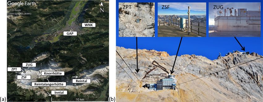
correction factor ADVS-selected data. Figure 2a shows the CO2 time series
G = 0.956 + 0.00017 · CZPT (1) before and after ADVS data selection. We also evaluated the
starting time windows resulting from ADVS data selection
was applied to the ZPT data, where CZPT denotes the CO2 with the detrended mean diurnal cycles as described in Yuan
concentrations at ZPT. Because of the same calibration mix- et al. (2018) for each measurement site in Fig. 2b. The num-
tures, an additional adjustment was applied to the CO2 con- ber of ADVS-selected data is summarized as percentage per
Atmos. Chem. Phys., 19, 999–1012, 2019 www.atmos-chem-phys.net/19/999/2019/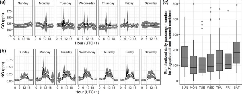
Y. Yuan et al.: Weekly, seasonal cycles and annual trends in atmospheric CO2 at Mount Zugspitze 1003
Table 1. Detailed description of atmospheric CO2 measurement techniques (NDIR is the nondispersive infrared, GC is gas chromatography,
and CRDS is cavity ring-down spectroscopy). At ZSF, CO2 data from GC measurements were not available from 2012 to 2013 due to an
instrumental failure; thus data from CRDS measurements were used in these 2 years for this study. However, CRDS measurements were
performed in parallel from the same air inlet from 2011.
ID Time period Instrument (analytical method) Scale Calibration gas
ZPT 1981–1997 1981–1984: Hartmann & Braun URAS 2 (NDIR) WMO X74 scale CO2 in N2
1985–1988: Hartmann & Braun URAS 2T (NDIR)
1989–1997: Hartmann & Braun URAS 3G (NDIR)
ZUG 1995–2001 Hartmann & Braun URAS 3G (NDIR) WMO X85 scale CO2 in natural air
ZSF 2001–2016 2001–2016: Hewlett Packard Modified HP 6890 WMO X2007 scale CO2 in natural air
Chem. station (GC)
2012–2013: Picarro EnviroSense 3000i (CRDS)
WNK 1981–1996 Hartmann & Braun URAS 2T (NDIR) WMO X74 scale CO2 in N2
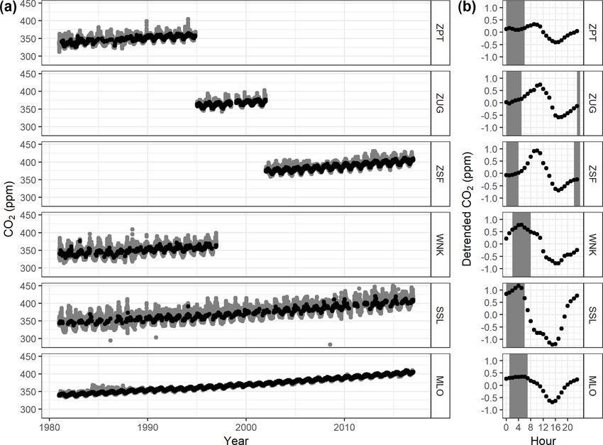
Figure 2. (a) Time series plot of 30-min averaged CO2 concentrations measured at Mount Zugspitze (ZPT, ZUG, and ZSF) and Wank
(WNK), and hourly averaged CO2 concentrations measured at Schauinsland (SSL) and Mauna Loa (MLO) with ADVS selection. Grey and
black colors are used for the unselected and selected results. (b) Detrended mean diurnal cycles with starting time windows (in grey) for
ADVS data selection.
hour in the total number of all CO2 data in Fig. 3. A detailed gle day. Additionally, only the MSR values with no data gaps
description and discussion is given in Sect. 3.1. in all the seven differences are considered as valid. Finally,
all the MSR values are aggregated into overall mean values
2.5 Mean symmetrized residual for each day of the week. In addition, the MSR values are
standardized so that the sum of all the seven values is equal
Weekly periodicity was calculated using the mean sym- to 0 (Cerveny and Coakley, 2002).
metrized residual (MSR) method, which was originally ap-
plied to atmospheric CO2 data (Cerveny and Coakley, 2002). 2.6 STL decomposition
The MSR method focuses on variations in mean values for
the days of the week. Daily deviations from the 7-day (con- The seasonal-trend decomposition technique (STL) was ap-
secutive) averages are calculated without ADVS selection to plied to decompose the CO2 time series into trend, sea-
account for the most likely emission cycles. Then, the MSR sonal, and remainder components individually (Cleveland
values are derived by averaging the differences for each sin- et al., 1983, 1990), which, in previous studies, has been
www.atmos-chem-phys.net/19/999/2019/ Atmos. Chem. Phys., 19, 999–1012, 2019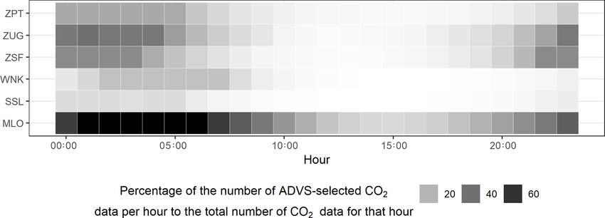
1004                  Y. Yuan et al.: Weekly, seasonal cycles and annual trends in atmospheric CO2 at Mount Zugspitze

a commonly applied method (e.g., Stephens et al., 2013;           3     Results and discussion
Hernández-Paniagua et al., 2015). Locally weighted polyno-
mial regressions were iteratively fitted to all monthly values    3.1    ADVS selection and diurnal variation
in both an outer and an inner loop. According to Cleveland
et al. (1990) and Pickers and Manning (2015), we set the          The resulting ADVS-selected CO2 data showed a clear link-
trend and seasonal smoothing parameters to 25 and 5, respec-      age of the percentage of selected data and the altitude of the
tively. The CO2 time series at each site or location were ag-     measurement site. Among the continental stations, the per-
gregated into monthly averages and, then, decomposed using        centage increased with altitude. A lower percentage indicates
STL. Missing monthly values were substituted using spline         higher data variability due to lower elevation and proxim-
interpolation.                                                    ity to local sources and sinks. At Schauinsland, the percent-
   To study the trend and seasonality, we firstly intended to     age of CO2 data by the ADVS selection was 6.3 %, while
apply STL decomposition to the ADVS-selected time series.         the percentages at Mount Zugspitze reached 9.9 % (ZPT),
However, due to multiple occurrences of consecutively miss-       19.5 % (ZUG), and 13.6 % (ZSF), respectively. A moderate
ing values in the ADVS-selected monthly averages, espe-           percentage of 6.3 % was also derived at Mount Wank. How-
cially for measurement sites at lower elevations (WNK and         ever, regarding the elevated mountain station Mauna Loa on
SSL), it was more practical to use the original CO2 time se-      the island of Hawaii, a much higher percentage (40.0 %) of
ries without ADVS data selection for STL decomposition, to        CO2 data was selected using ADVS as being representative
preserve time series continuity (Pickers and Manning, 2015).      of its background concentration, mainly due to the very lim-
There is one missing 6-month time interval at ZUG in 1998         ited nearby anthropogenic sources as well as mostly clean,
(July to December). Thus STL was performed separately for         well-mixed air arriving there. A similar result for an island
the time periods before (January 1995–June 1998) and af-          mountain station can be found in Yuan et al. (2018), in which
ter (January 1999–December 2001) the gap. Nevertheless,           a percentage of 36.2 % was computed for the CO2 measure-
we still applied STL decomposition to the ADVS-selected           ments at Izaña station on the island of Tenerife (28◦ 190 N,
data sets from Mount Zugspitze and Mauna Loa, since these         16◦ 300 E; 2373 m a.s.l.). This can also be explained by the
selected time series were applicable. At ZPT, due to larger       detrended mean diurnal cycles shown in Figs. 2b and 3. The
time gaps of missing data at the beginning (1981 and 1982)        mean diurnal cycle at MLO only exhibits a clear trough dur-
of the ADVS-selected data set, the ADVS-selected and STL-         ing daytime, especially starting from 12:00 local time (LT),
decomposed results were only studied starting from 1983. In-      which is believed to be influenced by the vegetation activ-
dividual figures of each STL-decomposed component at all          ity (photosynthesis) in the surroundings. The same effect can
stations can be found in the Supplement.                          be seen at WNK and SSL, but with larger magnitudes and
   For annual growth rates we did not include the WNK             earlier occurrences of the minima because of their lower lo-
time series due to shorter time periods of available data.        cations closer to CO2 sinks. In contrast, at these two sites the
Monthly trend components were first aggregated into annual        CO2 maxima in the diurnal cycles were not as clearly notice-
mean values. Then, the annual CO2 growth rates were cal-          able as at Mount Zugspitze due to anthropogenic sources and
culated as the difference between the CO2 value of the cur-       high biogenic respiration. At the three locations on Mount
rent year and the value from the previous year (Jones and         Zugspitze, the CO2 peaks in the mean diurnal cycles are
Cox, 2005). The mean seasonal cycle was aggregated di-            driven by the late-morning convective upslope wind, which
rectly from the monthly seasonal components by month. To          was relatively obvious at both ZUG and ZSF. However, from
observe potential deviations on the regional and global scale,    the perspective of data selection, a significantly higher per-
we compared the trend and seasonality derived from the            centage of CO2 data was selected at ZSF compared with ZPT,
STL-decomposed components at Zugspitze with other mea-            although there is only a small difference in altitude of around
surement sites. We included the globally averaged marine          only 70 m. This proves that ZSF is capable of capturing more
surface monthly mean data from NOAA (https://www.esrl.            background conditions than ZPT during the day. Neverthe-
noaa.gov/gmd/ccgg/trends/; last access: 23 January 2019)          less, based on the starting time window computed for ADVS
and data for the global mean mole fractions from WDCGG            selection, we found that, in general, most stations exhibited
(WMO Greenhouse Gas Bulletin, 2018) as references, and            similar starting time windows beginning around midnight,
processed these data based on the identical STL decomposi-        and the ADVS data selection was applied systematically by
tion routine. All the statistical analyses described above (in-   including more data around these hours (see Fig. 3), which
cluding ADVS, MSR, and STL) were performed in the R               confirmed our assumption of background conditions during
environment (R Core Team, 2018).                                  midnight for the ADVS data selection (Yuan et al., 2018).

                                                                  3.2    Weekly periodicity

                                                                  For a better characterization of the differences among the
                                                                  measurement locations at Mount Zugspitze, the mean CO2

Atmos. Chem. Phys., 19, 999–1012, 2019                                               www.atmos-chem-phys.net/19/999/2019/
Y. Yuan et al.: Weekly, seasonal cycles and annual trends in atmospheric CO2 at Mount Zugspitze 1005 Figure 3. Frequency of the percentages of the number of ADVS-selected CO2 data for each hour (0 to 23) in the total number of CO2 data for that hour as shown in greyscale. Figure 4. (a) Mean MSR CO2 values at Mount Zugspitze and MLO as a function of the day of the week. Mean MSR values are adjusted such that they sum to 0. (b) Detrended mean CO2 diurnal cycles at ZSF by day of the week from 2002 to 2016. Uncertainties at the 95 % confidence interval are shown by the shaded areas. weekly cycles were analyzed as a function of mean MSR on working days and minimum ratios on Sundays at neigh- values (see Fig. 4a). The mean MSR values at the MLO boring stations were observed, generally suggesting an an- for the corresponding time intervals were also calculated. thropogenic impact at all elevations. Most weekly cycles exhibited no clear peaks or patterns for We obtained more insights into the weekly CO2 cycle at both sites. However, the magnitude of MSR data variability Mount Zugspitze by comparing the mean diurnal cycles of is mostly higher at Zugspitze, with a maximum on Thurs- weekdays and weekends (see Fig. 4b). Detrended mean diur- days. The only significant weekday–weekend difference is nal cycles at ZSF, from Sunday to Saturday, were calculated observed at ZSF in terms of the 95 % confidence interval, by subtracting the daily averages from the daily data between which shows weekly maxima and weekly minima on Thurs- 2002 and 2016. In the morning around 09:00 to 10:00 LT the day and Saturday, respectively (peak-to-trough difference: CO2 levels at ZSF are higher on weekdays than weekends, 0.76 ppm). Gilge et al. (2010) observed similar phenomena while CO2 diurnal patterns during the rest of the week are when studying O3 and NO2 concentrations at Alpine moun- relatively stable. Such weekly cycles are not observable at tain stations, including Zugspitze. Clear weekly cycles, with ZPT and ZUG, nor at WNK and SSL (see Fig. S18). At ZPT, enhanced O3 levels on working days, were observed at ZSF there are fewer variations in the diurnal cycle compared to in summer, with weekly maxima and minima on Thursdays ZSF, indicating that this location does not receive the effect and Sundays, respectively. For NO2 , maximum mixing ratios of regular local anthropogenic working activities and hence it www.atmos-chem-phys.net/19/999/2019/ Atmos. Chem. Phys., 19, 999–1012, 2019
1006                  Y. Yuan et al.: Weekly, seasonal cycles and annual trends in atmospheric CO2 at Mount Zugspitze

is more representative of lower free tropospheric conditions      identical value of 1.8 ppm yr−1 . Then, we divided the entire
regarding this aspect. The weekday–weekend differences at         time period (1981–2016) into three time blocks, correspond-
ZSF are possibly due to local working patterns, whereas the       ing to the different locations at Mount Zugspitze, in order to
absence of this pattern at lower sites may indicate influences    observe potential differences with respect to other sites sep-
from a more regional reservoir. In fact, ZSF is closed on the     arately (see Table 2). The results show good agreement of
weekends and, thus, is influenced by less immediate anthro-       each location on Mount Zugspitze with other measurement
pogenic activities.                                               sites (also for the ADVS-selected results) as well as a clearly
                                                                  increasing trend of the annual growth rates over these three
3.3    Case study on atmospheric CO and NO and                    time blocks. Only the mean annual growth rate between 1995
       passenger numbers at Zugspitze                             and 2001 at ZUG is obviously lower than at the other sites.
                                                                  This can be explained by the missing monthly values in 1998,
To study the potential sources and sinks for such weekday–        and thus in turn the annual growth rates of 1998 and 1999
weekend differences in the CO2 diurnal cycles at ZSF fur-         were left out for the average. However, the annual growth
ther, we analyzed atmospheric CO and NO data at ZSF and           rates of these 2 years reached anomalous peaks at most sites
the daily combined number of cable car and train passengers       (see details later in Sect. 3.6). Möller (2017) also mentioned
to Zugspitzplatt and to the Zugspitze summit in 2016. At-         that 1981 to 1992 growth rates at both German stations and
mospheric CO and NO are known to be good indicators of            MLO were identical.
local anthropogenic influences due to highly variable short-
term signals and are thus helpful to identify potential CO2       3.5   Seasonality
sources (Tsutsumi et al., 2006; Sirignano et al., 2010; Wang
et al., 2010; Liu et al., 2016). In this study, we used at-       For the overall seasonality, Fig. 6 presents the mean seasonal
mospheric NO due to its short lifetime based on rapid at-         cycles for the STL-decomposed seasonal components. We
mospheric NO2 formation with resulting altitude-dependent         observed similar patterns in the SSL and WNK seasonal cy-
O3 surplus, indicating the presence of sources at closer dis-     cles, with mean peak-to-trough amplitudes of 15.9 ± 1.0 and
tances. The CO and NO data shown in Fig. 5 include data that      15.9±1.5 ppm, respectively. The composite data set at Mount
were flagged during data processing because for the deliv-        Zugspitze results in a lower amplitude (12.4 ± 0.6 ppm),
ery to GAW World Data Centres the logged and recognized           but still exhibits a similar seasonality influenced by ac-
work-dependent concentration peaks are flagged. A clear           tive biogenic processes (mainly photosynthesis) in summer
weekday–weekend difference is observed for both CO and            compared with SSL and WNK (Dettinger and Ghil, 1998).
NO. Only weekdays are characterized by multiple short-term        As vegetation grows with rising temperatures (approaching
atmospheric CO events and higher atmospheric NO peaks             summer), CO2 levels decrease due to more and more intense
during the daytime (mostly around 09:00 LT), which fits per-      photosynthetic activities till a minimum in August. In addi-
fectly with daytime peaks in CO2 diurnal cycles. A general        tion, with rising temperatures, locally influenced air masses
fluctuating pattern in NO throughout the week is thought          reach Mount Zugspitze more often due to “Alpine pumping”
to originate from heating of the Zugspitzplatt and changing       (Carnuth et al., 2002; Winkler et al., 2006). As such, air sam-
work with combustion engines. On the other hand, the daily        pled in summer is more frequently mixed with air from lower
number of passengers at Zugspitze (see Fig. 5c) shows a clear     levels, which is characterized by lower CO2 concentrations,
weekday–weekend pattern, with a higher number of passen-          intensifying the August minimum. Anthropogenic activities
gers on the weekends. However, increased numbers of pas-          and plant respiration dominate the increases in concentration
sengers on the weekends do not correspond to higher levels        in the winter (January to April). This influence appears to be
of CO and CO2 , indicating that measured CO2 levels are not       stronger at SSL and WNK than at Mount Zugspitze. Lower
significantly influenced by tourist activities nearby. Instead,   levels of CO2 and a 1-month delay, from February to March,
it is more likely that anthropogenic working activities are the   of the seasonal maximum at Mount Zugspitze are in agree-
main driver of weekly periodicity.                                ment with the expectation of thermally driven orographic
                                                                  processes that drive the upward transport of CO2 from local
3.4    Trend                                                      sources, as well as limited human access to Mount Zugspitze
                                                                  and the prevailing absence of biogenic activities at such high
Based on the STL-decomposed results, the mean annual              elevations. Regarding the resulting seasonal cycles based on
growth rate of the 36-year composite record at Mount              ADVS-selected Zugspitze data sets, similar patterns were ob-
Zugspitze from the three measurement locations is 1.8 ±           served but with a lower amplitude (10.5 ± 0.5 ppm) as well
0.4 ppm yr−1 , which is consistent with the SSL (1.8 ±            as a 2-month shift of the seasonal maximum to April.
0.4 ppm yr−1 ), MLO (1.8 ± 0.2 ppm yr−1 ), and global means          The Mauna Loa CO2 record is characterized by a sea-
(NOAA: 1.8 ± 0.2 ppm yr−1 ; WDCGG: 1.8 ± 0.2 ppm yr−1 ).          sonal maximum in May and a minimum in September, with
The mean annual growth rates from the ADVS-selected data          a peak-to-trough amplitude of 6.8 ± 0.1 ppm, which agrees
sets at Mount Zugspitze and Mauna Loa also result in the          with observations from Dettinger and Ghil (1998) and Lint-

Atmos. Chem. Phys., 19, 999–1012, 2019                                                www.atmos-chem-phys.net/19/999/2019/
Y. Yuan et al.: Weekly, seasonal cycles and annual trends in atmospheric CO2 at Mount Zugspitze 1007
Figure 5. Mean diurnal plots at ZSF during 2016 by day of the week for (a) CO and (b) NO, and (c) the standardized daily passenger number
at the Zugspitzplatt and Zugspitze summit combined.
Table 2. Mean annual CO2 growth rates in ppm yr−1 at the 95 % confidence interval based on three time blocks for all measurement
sites/locations studied (SSL – Schauinsland; WNK – Mount Wank; ZPT – pedestrian tunnel at Mount Zugspitze; ZUG – Zugspitze summit;
ZSF – Zugspitze Schneefernerhaus; MLO – Mauna Loa; WDCGG and NOAA – global means). ADVS means the data were selected using
the ADVS method. This comparison refers to data from all years including the corresponding time period for all stations. Measurement sites
or locations where data are not available for calculating the corresponding time blocks are shown by “–”.
Time SSL WNK ZPT ZPT ZUG ZUG ZSF ZSF MLO MLO WDCGG NOAA
block ADVS ADVS ADVS ADVS
1981–1994 1.5 ± 0.5 1.4 ± 1.1 1.5 ± 0.8 1.5 ± 1.4 – – – – 1.4 ± 0.3 1.4 ± 0.3 1.4 ± 0.4 1.4 ± 0.3
1995–2001 1.7 ± 1.1 – – – 1.3 ± 0.8 1.5 ± 0.5 – – 1.8 ± 0.5 1.8 ± 0.5 1.8 ± 0.4 1.7 ± 0.5
2002–2016 2.2 ± 0.7 – – – – – 2.2 ± 0.4 2.2 ± 0.4 2.2 ± 0.2 2.2 ± 0.2 2.2 ± 0.2 2.2 ± 0.2
ical marine boundary layer (MBL) condition for the levels
of background CO2 in the atmosphere. On the other hand,
the WDCGG global mean includes continental characteris-
tics for its calculation, thus exhibiting a slightly more con-
tinental signature which can be equally seen in the seasonal
cycles at continental sites, such as Mount Zugspitze. April
and October appear to be the important months that indicate
the switch of either CO2 source to sinks or vice versa for the
continent.
We then examine in more detail the seasonal cycles at ZPT,
ZUG, and ZSF. Despite the close proximity, there are dif-
ferences in their seasonal amplitudes (ZPT: 11.9 ± 1.2 ppm;
ZUG: 11.2 ± 1.0 ppm; ZSF: 13.3 ± 0.7 ppm). Good agree-
Figure 6. Mean CO2 seasonal cycles from the STL seasonal com- ment is shown between CO2 seasonal cycles from April to
ponent at each measurement site or location. Uncertainties at the June and from October to December. However, significantly
95 % confidence interval are shown by the shaded areas with corre- higher levels of CO2 were evident at ZSF from January to
sponding colors. March as well as lower levels from July to September. After
data selection with lower seasonal amplitudes of 10.3 ± 1.3
(ZPT_ADVS), 10.3±1.2 (ZUG_ADVS), and 10.9±0.6 ppm
(ZSF_ADVS), similar differences of the CO2 levels in the
ner et al. (2006). The ADVS-selected results for MLO also seasonal cycles could be observed. These results indicate
show a similar pattern, with a lower amplitude of 6.6 ± that factors such as elevation and measurement surround-
0.1 ppm. Global means exhibited the lowest seasonal ampli- ings strongly determine the air-mass composition via local
tudes, 4.4 ± 0.1 ppm (NOAA) and 4.8 ± 0.0 ppm (WDCGG). vertical transport. The amount of air-mass transport via oro-
Compared with WDCGG, the NOAA global mean better fits graphic lifting affects the three locations differently. The
the seasonal cycle of MLO supporting the presence of a typ-
www.atmos-chem-phys.net/19/999/2019/ Atmos. Chem. Phys., 19, 999–1012, 20191008 Y. Yuan et al.: Weekly, seasonal cycles and annual trends in atmospheric CO2 at Mount Zugspitze
lower elevation station, ZSF, apparently captures more mixed CO2 due to daily, local anthropogenic sources during win-
air masses due to a daytime up-valley flow along the Reintal ter and convective upwind transport during seasons without
(Gantner et al., 2003) as well as a slightly southeastern flow snow cover that are characterized by lower concentrations
from the Inntal (see Fig. 1) that is less frequent for the higher of CO2 at lower altitudes. Such patterns in the data are also
locations (ZPT or ZUG). In addition, comparably postponed evident in the annual growth rates and seasonal amplitudes.
seasonal maxima at ZUG and ZPT from March to April The overall patterns at Mount Zugspitze agree with SSL and
show delayed onset of convective upwind air-mass transport WNK. However, SSL and WNK exhibit more variation in
and changing planetary boundary layer (PBL) compositions. the annual growth rates and higher seasonal amplitude lev-
On the other hand, these differences in the seasonal ampli- els (see Fig. 7b and c). In addition, slightly higher seasonal
tudes (even though not significant at the 95 % confidence in- amplitudes for the WDCGG global mean compared with the
terval) might be influenced by a potential trend in the sea- NOAA one can be explained by the WDCGG global mean
sonal amplitude over time. Such increasing trends of the sea- calculation method, which includes more continental stations
sonal CO2 amplitudes (i.e., +0.32 % yr−1 at Mauna Loa and (WMO Greenhouse Gas Bulletin, 2018).
+0.60 % yr−1 at Utqiaġvik, formerly Barrow, Alaska) were Anomalies in the annual growth rates are frequently ob-
studied in Graven et al. (2013), indicating an enhanced inter- served, which are possibly explained by climatic influences
action between the biospheric and atmospheric CO2 across such as the El Niño–Southern Oscillation (ENSO), volcanic
the Northern Hemisphere. activity, and extreme weather conditions (Keeling et al.,
1995; Jones and Cox, 2001; Francey et al., 2010; Keenan
3.6 Interannual variation et al., 2016). One of the largest positive annual growth rate
anomalies occurred in 1998 and is clearly seen in all the
To study the interannual variability, we focused on the per- records (aside from ZUG with missing values), which is at-
centages of ADVS selection, the growth rates, and the sea- tributed to a strong El Niño event (Watanabe et al., 2000;
sonal amplitudes. The annual percentages from ADVS data Jones and Cox, 2005). Similar signals are found in 1988, es-
selection are shown for years without missing monthly av- pecially at MLO and in global means. Such anomalies are
erages (see Fig. 7a). An exceptionally high percentage at more clearly observed in the global and seaside time se-
Zugspitze in 2000 resulted from careful and intensive filter- ries. Regarding continental sites, interannual signals may be
ing of the original CO2 data. The total number of original hidden by more intense land influences rather than global
validated 30 min data points in 2000 is only 4634, while the effects. Moreover, positive consecutive anomalies between
number of data for other years ranges from 8754 to 15 339 2002 and 2003 are clearly observed at ZSF and SSL, which
(except for 1998, with only 6-month data, the total number are potentially due to anomalous climatic conditions, such
of 30 min CO2 data is 6441). As described in the previous as the dry European summer in 2003 that led to an increas-
section, the annual growth rates are plotted in Fig. 7b. The ing number of forest fires. These events are also observ-
annual CO2 seasonal amplitudes are calculated as the differ- able in the MLO and global means but at a smaller scale
ence between the yearly maximum and minimum monthly (Jones and Cox, 2005). At all German sites, clear negative
CO2 values from the STL-decomposed seasonal components anomalies, due to violent eruptions of the El Chichón and
(see Fig. 7c). Mt. Pinatubo volcanoes and the subsequent volcanic-induced
Focusing on the annual percentages from ADVS-selected surface cooling effect are observed after stratospheric aerosol
representative data after 1990, we calculated the mean an- maxima above Garmisch-Partenkirchen in 1983 and 1992,
nual percentages at Mount Zugspitze locations, for the time respectively (Lucht et al., 2002; Frölicher et al., 2011, 2013;
periods between 1990 and 2001 (2000 was not included for Trickl et al., 2013). This effect is only slightly visible in the
ZUG) and 2002 and 2016. We observe significantly higher MLO and global means despite the fact that volcanic aerosols
percentages at ZPT and ZUG (18.5 ± 2.4 %) than at ZSF spread over the entire globe.
(13.6±1.1 %) at the 95 % confidence interval. These percent- However, the reasons for some anomalies are still unclear.
ages are different from SSL (4.2±0.5 % vs. 4.2±0.6 %) and These include the negative anomalies during 1985 and 1986
MLO (43.5 ± 1.4 % vs. 42.1 ± 1.6 %). A likely explanation at all Germans sites. Certain anomalies in the annual per-
is that there are systematically different air-mass transport centages and seasonal amplitudes also derive from extremely
characteristics reaching each of these locations. Higher per- low ADVS selection percentages beginning in 1984 and con-
centages at ZPT and ZUG indicate that these locations are tinuing until 1990, with peaks in seasonal amplitudes be-
capable of capturing more air masses that have traveled over tween 1985 and 1986. This is the reason why we calculated
long distances along the mountains. These air masses trap the mean annual ADVS selection percentage beginning at
air that ascends from many Alpine valleys, but also from re- 1990. We assume that local influences mask similar physical
mote source regions up to the intercontinental scale (Trickl mechanisms at the sites. However, annual percentages at the
et al., 2003; Huntrieser et al., 2005). On the other hand, MLO also have similar characteristics. Therefore, it is still
ZSF is dominated by mixing air masses that have traveled unclear what triggers such distinct interannual data variabil-
along the Zugspitzplatt area, which contain higher levels of ity across measurement sites. Another clear negative annual
Atmos. Chem. Phys., 19, 999–1012, 2019 www.atmos-chem-phys.net/19/999/2019/Y. Yuan et al.: Weekly, seasonal cycles and annual trends in atmospheric CO2 at Mount Zugspitze 1009
Figure 7. (a) Annual ADVS-selected percentages. (b) Annual CO2 growth rates and global means from the NOAA and the WDCGG. The
calculated growth rates are shown at the beginning of the year. Since the time period starts in 1981, the values of growth rates start in 1982.
WDCGG data are only available starting in 1984. (c) Annual CO2 seasonal amplitudes.
growth rate anomaly occurred in 2014 across all sites. Such However, several anomalies still exist across most stations
anomalies still require further investigation, but are beyond that lack clear explanations. These anomalies require further
the scope of this study. investigation, possibly by analyzing correlations between ex-
treme events and historical meteorological or hydrological
data. Finally, we conclude that, at Zugspitze, we cannot ne-
4 Conclusions glect local to regional influences. Regarding the seasonal am-
plitude, Mount Zugspitze is significantly more influenced
In this study, we presented a time series analysis of a 36-year by biogenic activity, mostly in the summer, compared with
composite CO2 measurement record at Mount Zugspitze in Mauna Loa and global means. On the other hand, the weekly
Germany, together with a thorough study of the weekly pe- periodicity analysis provides a clear picture of local CO2
riodicity combined with diurnal cycles. Even though it is sources that potentially result from human working activi-
challenging to quantify local sources and sinks, this study ties, especially at ZSF. Overall, this study provides detailed
shows that it is possible to gain information on variation in insights into long-term atmospheric CO2 measurements, as
this regard. Compared with the GAW regional observatories well as site characteristics at Mount Zugspitze. We propose
at Schauinsland and Wank Peak, as well as the GAW global the application of this type of analysis as a systematic tool for
observatory at Mauna Loa, Mount Zugspitze proves to be a the physical and quantitative classification of stations with
highly suitable site for monitoring the background levels of respect to their lower free tropospheric representativeness.
air components using proper data selection procedures. The As an additional component in this analysis, weekly period-
long-term trend at Zugspitze agrees well with that at Mauna icity can be used to analyze anthropogenic influences. The
Loa and global means. The seasonality and short-term vari- systematic application of this approach to larger continen-
ations show similar patterns, but are considerably less influ- tal or global regions can serve as a basis for more quantita-
enced by local to regional mechanisms than the lower ele- tive analyses of global greenhouse gases trends such as CO2 .
vation stations at Schauinsland and Wank Peak. Interannual Based on the physical foundation of the methodology pre-
variations also correlate well with anomalous global events.
www.atmos-chem-phys.net/19/999/2019/ Atmos. Chem. Phys., 19, 999–1012, 20191010 Y. Yuan et al.: Weekly, seasonal cycles and annual trends in atmospheric CO2 at Mount Zugspitze
sented here, we suggest that these techniques can be applied IMK-IFU for his high-quality data measurement until 2001 at the
to other greenhouse gases such as SF6 , CH4 , and aerosols. Zugspitze Summit (ZUG). For a long period, Hans-Eckhart Scheel,
who passed away in 2013, led the in situ measurement program at
the Zugspitze summit with a high level of expertise and diligence.
Data availability. NOAA global mean data are available at ftp: Former IFU staff members helped us to reconstruct details of
//aftp.cmdl.noaa.gov/products/trends/co2/co2_mm_gl.txt (last ac- the measurements. We would also like to thank the operating
cess: 23 January 2019). team at the Environmental Research Station Schneefernerhaus for
WDCGG global mean data are available at https://gaw.kishou.go. supporting our scientific activities and the Bavarian Ministry for
jp/publications/global_mean_mole_fractions (WDCGG, 2019a). Environment for supporting this High Altitude Research Station.
CO2 records (also including CO and NO) of all GAW observato- Finally, our gratitude goes to the Bavarian Zugspitze railway
ries which were used in this study are available from the World Data company for the passenger data for 2016.
Centre for Greenhouse Gases (WDCGG) at https://gaw.kishou.go.
jp/ (WDCGG, 2019b). This work was supported by the German Research
The daily passenger number data for Zugspitze were provided by Foundation (DFG) and the Technical University of Munich (TUM)
the Bayerische Zugspitzbahn railway company. in the framework of the Open Access Publishing Program.
Edited by: Rachel Law
Reviewed by: two anonymous referees
Supplement. The supplement related to this article is available
online at: https://doi.org/10.5194/acp-19-999-2019-supplement.
References
Author contributions. YY, LR, HP, and AM designed the study and
YY performed the data analyses with help from LR and HP for Bader, J.: Aufbau und Betrieb eines automatisierten Gaschro-
the data processing and code validation. Atmospheric measurement matographen HP 6890 zur kontinuierlichen Messung von CO2 ,
data were collected, preprocessed, and provided by LR, TT, CC, RS, CH4 , N2 O und SF6 , Universität Heidelberg, 2001.
and FM. Information about data quality assurance and measurement Beardsmore, D. J. and Pearman, G. I.: Atmospheric carbon dioxide
site was provided by LR. YY prepared the manuscript with contri- measurements in the Australian region: Data from surface ob-
butions from all co-authors. servatories, Tellus B, 39, 42–66, https://doi.org/10.1111/j.1600-
0889.1987.tb00269.x, 1987.
Bischof, W.: The influence of the carrier gas on the in-
Competing interests. The authors declare that they have no conflict frared gas analysis of atmospheric CO2 , Tellus, 27, 59–61,
of interest. https://doi.org/10.3402/tellusa.v27i1.9884, 1975.
Bousquet, P., Gaudry, A., Ciais, P., Kazan, V., Monfray, P., Sim-
monds, P. G., Jennings, S. G., and O’Connor, T. C.: Atmo-
Special issue statement. This article is part of the special issue spheric CO2 concentration variations recorded at Mace Head,
“The 10th International Carbon Dioxide Conference (ICDC10) and Ireland, from 1992 to 1994, Phys. Chem. Earth, 21, 477–481,
the 19th WMO/IAEA Meeting on Carbon Dioxide, other Green- https://doi.org/10.1016/S0079-1946(97)81145-7, 1996.
house Gases and Related Measurement Techniques (GGMT-2017) Carnuth, W. and Trickl, T.: Transport studies with the
(AMT/ACP/BG/CP/ESD inter-journal SI)”. It is a result of the IFU three-wavelength aerosol lidar during the VOTALP
19th WMO/IAEA Meeting on Carbon Dioxide, Other Greenhouse Mesolcina experiment, Atmos. Environ., 34, 1425–1434,
Gases, and Related Measurement Techniques (GGMT-2017), Empa https://doi.org/10.1016/S1352-2310(99)00423-9, 2000.
Dübendorf, Switzerland, 27–31 August 2017. Carnuth, W., Kempfer, U., and Trickl, T.: Highlights of the tropo-
spheric lidar studies at IFU within the TOR project, Tellus B,
54, 163–185, https://doi.org/10.1034/j.1600-0889.2002.00245.x,
Acknowledgements. This study was supported by a scholarship 2002.
from the China Scholarship Council (CSC) under grant CSC Cerveny, R. S. and Coakley, K. J.: A weekly cycle in atmo-
no. 201508080110. We acknowledge support from a MICMoR spheric carbon dioxide, Geophys. Res. Lett., 29, 15-1–15-4,
fellowship through the KIT/IMK-IFU to Ye Yuan. Our thanks go https://doi.org/10.1029/2001GL013952, 2002.
to Gourav Misra for the geographical map of the measurement Ciattaglia, L.: Interpretation of atmospheric CO2 measurements at
locations. Our thanks go to James Butler and Kirk Thoning from Mt. Cimone (Italy) related to wind data, J. Geophys. Res., 88,
NOAA for their indispensable discussions on the problematic 1331, https://doi.org/10.1029/JC088iC02p01331, 1983.
nature of representing and comparing data on different older and Cleveland, R. B., Cleveland, W. S., McRae, J. E., and Terpenning, I.:
current CO2 scales. The CO2 , CO, and NO measurements at STL: A seasonal-trend decomposition procedure based on loess,
Zugspitze Schneefernerhaus and at Platform Zugspitze of the GAW J. Off. Stat., 6, 3–73, 1990.
global observatory Zugspitze/Hohenpeissenberg and CO2 measure- Cleveland, W. S., Freeny, A. E., and Graedel, T. E.:
ments at Schauinsland are supported by the German Environment The seasonal component of atmospheric CO2 : Infor-
Agency (UBA). The IMK-IFU provided data from the Zugspitze mation from new approaches to the decomposition
tunnel and summit. Our thanks go to Hans-Eckhart Scheel from the of seasonal time series, J. Geophys. Res., 88, 10934,
https://doi.org/10.1029/JC088iC15p10934, 1983.
Atmos. Chem. Phys., 19, 999–1012, 2019 www.atmos-chem-phys.net/19/999/2019/Y. Yuan et al.: Weekly, seasonal cycles and annual trends in atmospheric CO2 at Mount Zugspitze 1011 Cundari, V., Colombo, T., Papini, G., Benedicti, G., and Ciattaglia, and surface observations, J. Geophys. Res., 110, D01305, L.: Recent improvements on atmospheric CO2 measurements at https://doi.org/10.1029/2004JD005045, 2005. Mt. Cimone observatory, Italy, Il Nuovo Cimento C, 13, 871– Jones, C. D. and Cox, P. M.: Modeling the volcanic signal in the 882, https://doi.org/10.1007/BF02512003, 1990. atmospheric CO2 record, Global Biogeochem. Cy., 15, 453–465, Dettinger, M. D. and Ghil, M.: Seasonal and interannual vari- https://doi.org/10.1029/2000GB001281, 2001. ations of atmospheric CO2 and climate, Tellus B, 50, 1–24, Jones, C. D. and Cox, P. M.: On the significance of atmospheric https://doi.org/10.1034/j.1600-0889.1998.00001.x, 1998. CO2 growth rate anomalies in 2002–2003, Geophys. Res. Lett., Francey, R. J., Trudinger, C. M., van der Schoot, M., Krum- 32, L14816, https://doi.org/10.1029/2005GL023027, 2005. mel, P. B., Steele, L. P., and Langenfelds, R. L.: Differ- Keeling, C. D., Adams, J. A., Ekdahl, C. A., and Guen- ences between trends in atmospheric CO2 and the reported ther, P. R.: Atmospheric carbon dioxide variations at the trends in anthropogenic CO2 emissions, Tellus B, 62, 316–328, South Pole, Tellus, 28, 552–564, https://doi.org/10.1111/j.2153- https://doi.org/10.1111/j.1600-0889.2010.00472.x, 2010. 3490.1976.tb00702.x, 1976. Frölicher, T. L., Joos, F., and Raible, C. C.: Sensitivity of atmo- Keeling, C. D., Whorf, T. P., Wahlen, M., and van der spheric CO2 and climate to explosive volcanic eruptions, Bio- Plichtt, J.: Interannual extremes in the rate of rise of at- geosciences, 8, 2317–2339, https://doi.org/10.5194/bg-8-2317- mospheric carbon dioxide since 1980, Nature, 375, 666–670, 2011, 2011. https://doi.org/10.1038/375666a0, 1995. Frölicher, T. L., Joos, F., Raible, C. C., and Sarmiento, J. L.: Atmo- Keenan, T. F., Prentice, I. C., Canadell, J. G., Williams, C. spheric CO2 response to volcanic eruptions: The role of ENSO, A., Wang, H., Raupach, M., and Collatz, G. J.: Recent season, and variability, Global Biogeochem. Cy., 27, 239–251, pause in the growth rate of atmospheric CO2 due to en- https://doi.org/10.1002/gbc.20028, 2013. hanced terrestrial carbon uptake, Nat. Commun., 7, 13428, Gantner, L., Hornsteiner, M., Egger, J., and Hartjenstein, G.: The https://doi.org/10.1038/ncomms13428, 2016. diurnal circulation of Zugspitzplatt: Observations and mod- Le Quéré, C., Raupach, M. R., Canadell, J. G., Marland, G., Bopp, eling, Meteorol. Z., 12, 95–102, https://doi.org/10.1127/0941- L., Ciais, P., Conway, T. J., Doney, S. C., Feely, R. A., Foster, 2948/2003/0012-0095, 2003. P., Friedlingstein, P., Gurney, K., Houghton, R. A., House, J. I., Gilge, S., Plass-Duelmer, C., Fricke, W., Kaiser, A., Ries, L., Buch- Huntingford, C., Levy, P. E., Lomas, M. R., Majkut, J., Metzl, mann, B., and Steinbacher, M.: Ozone, carbon monoxide and N., Ometto, J. P., Peters, G. P., Prentice, I. C., Randerson, J. T., nitrogen oxides time series at four alpine GAW mountain sta- Running, S. W., Sarmiento, J. L., Schuster, U., Sitch, S., Taka- tions in central Europe, Atmos. Chem. Phys., 10, 12295–12316, hashi, T., Viovy, N., van der Werf, G. R., and Woodward, F. I.: https://doi.org/10.5194/acp-10-12295-2010, 2010. Trends in the sources and sinks of carbon dioxide, Nat. Geosci., Graven, H. D., Keeling, R. F., Piper, S. C., Patra, P. K., Stephens, 2, 831–836, https://doi.org/10.1038/ngeo689, 2009. B. B., Wofsy, S. C., Welp, L. R., Sweeney, C., Tans, P. P., Lintner, B. R., Buermann, W., Koven, C. D., and Fung, I. Y.: Sea- Kelley, J. J., Daube, B. C., Kort, E. A., Santoni, G. W., sonal circulation and Mauna Loa CO2 variability, J. Geophys. and Bent, J. D.: Enhanced seasonal exchange of CO2 by Res., 111, D13104, https://doi.org/10.1029/2005JD006535, northern ecosystems since 1960, Science, 341, 1085–1089, 2006. https://doi.org/10.1126/science.1239207, 2013. Liu, F., Beirle, S., Zhang, Q., Dörner, S., He, K., and Wagner, Griffith, D. W. T., Keeling, C. D., Adams, A., Guen- T.: NOx lifetimes and emissions of cities and power plants ther, P. R., and Bacastow, R. B.: Calculations of car- in polluted background estimated by satellite observations, At- rier gas effects in non-dispersive infrared analyzers. mos. Chem. Phys., 16, 5283–5298, https://doi.org/10.5194/acp- II. Comparisons with experiment, Tellus, 34, 385–397, 16-5283-2016, 2016. https://doi.org/10.3402/tellusa.v34i4.10825, 1982. Liu, Y., Gruber, N., and Brunner, D.: Spatiotemporal patterns Hammer, S., Glatzel-Mattheier, H., Müller, L., Sabasch, M., of the fossil-fuel CO2 signal in central Europe: results from Schmidt, M., Schmitt, S., Schönherr, C., Vogel, F., Wor- a high-resolution atmospheric transport model, Atmos. Chem. thy, D. E., and Levin, I.: A gas chromatographic sys- Phys., 17, 14145–14169, https://doi.org/10.5194/acp-17-14145- tem for high-precision quasi-continuous atmospheric measure- 2017, 2017. ments of CO2 , CH4 , N2 O, SF6 , CO and H2 , available Lucht, W., Prentice, I. C., Myneni, R. B., Sitch, S., Friedling- at: http://www.iup.uni-heidelberg.de/institut/forschung/groups/ stein, P., Cramer, W., Bousquet, P., Buermann, W., and Smith, kk/en/GC_Hammer_25_SEP_2008.pdf (last access: 23 January B.: Climatic control of the high-latitude vegetation green- 2019), 2008. ing trend and Pinatubo effect, Science, 296, 1687–1689, Hernández-Paniagua, I. Y., Lowry, D., Clemitshaw, K. C., Fisher, https://doi.org/10.1126/science.1071828, 2002. R. E., France, J. L., Lanoisellé, M., Ramonet, M., and Nisbet, Manning, M. R. and Pohl, K. P.: Atmospheric CO2 Monitoring in E. G.: Diurnal, seasonal, and annual trends in atmospheric CO2 New Zealand 1971-1985, Institute of Nuclear Sciences, DSIR, at southwest London during 2000–2012: Wind sector analysis New Zealand, Report No INS-R-350, 1986. and comparison with Mace Head, Ireland, Atmos. Environ., 105, McClure, C. D., Jaffe, D. A., and Gao, H.: Carbon Diox- 138–147, https://doi.org/10.1016/j.atmosenv.2015.01.021, 2015. ide in the Free Troposphere and Boundary Layer at the Mt. Huntrieser, H., Heland, J., Schlager, H., Forster, C., Stohl, Bachelor Observatory, Aerosol Air Qual. Res., 16, 717–728, A., Aufmhoff, H., Arnold, F., Scheel, H. E., Campana, https://doi.org/10.4209/aaqr.2015.05.0323, 2016. M., Gilge, S., Eixmann, R., and Cooper, O. R.: Intercon- Möller, D.: Chemistry of the climate system, 2nd fully revised and tinental air pollution transport from North America to Eu- extended edition, De Gruyter, Berlin, 786 pp., 2017. rope: Experimental evidence from airborne measurements www.atmos-chem-phys.net/19/999/2019/ Atmos. Chem. Phys., 19, 999–1012, 2019
You can also read