Environmental Regulations, Air and Water Pollution, and Infant Mortality in India
←
→
Page content transcription
If your browser does not render page correctly, please read the page content below
Environmental Regulations, Air and
Water Pollution, and Infant Mortality
              in India

     Michael Greenstone and Rema Hanna

July 2011                                                        CEEPR WP 2011-014

A Joint Center of the Department of Economics, MIT Energy Initiative and MIT Sloan School of Management.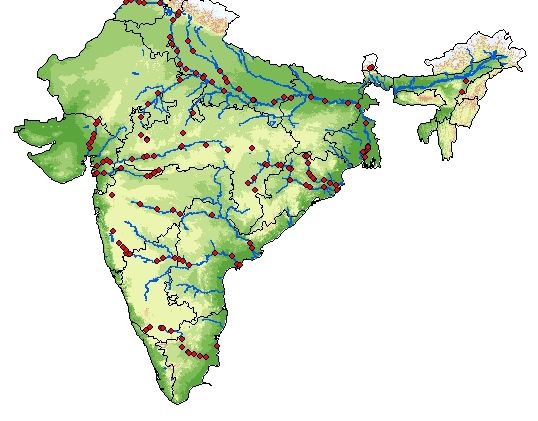
ENVIRONMENTAL REGULATIONS, AIR AND WATER POLLUTION, AND INFANT
                      MORTALITY IN INDIA

                                         Michael Greenstone
                                            Rema Hanna

                                            ABSTRACT

Using the most comprehensive data file ever compiled on air pollution, water pollution,
environmental regulations, and infant mortality from a developing country, the paper examines
the effectiveness of India’s environmental regulations. The air pollution regulations were
effective at reducing ambient concentrations of particulate matter, sulfur dioxide, and nitrogen
dioxide. The most successful air pollution regulation is associated with a modest and statistically
insignificant decline in infant mortality. However, the water pollution regulations had no
observable effect. Overall, these results contradict the conventional wisdom that environmental
quality is a deterministic function of income and underscore the role of institutions and politics.

Michael Greenstone                                              Rema Hanna
MIT Department of Economics                                     Kennedy School of Government
50 Memorial Drive, E52-359                                      Harvard University
Cambridge, MA 02142-1347                                        79 JFK Street
and NBER                                                        Cambridge, MA 02138
mgreenst@mit.edu                                                and NBER
                                                                rema_hanna@ksg.harvard.edu

We thank Samuel Stolper for truly outstanding research assistance. In addition, we thank Joseph Shapiro
and Abigail Friedman for excellent research assistance. Funding from the MIT Energy Initiative is
gratefully acknowledged. The analysis was conducted while Hanna was a fellow at the Science
Sustainability Program at Harvard University.

© 2011 by Michael Greenstone and Rema Hanna. All rights reserved. Short sections of text, not to exceed
two paragraphs, may be quoted without explicit permission provided that full credit, including © notice,
is given to the source.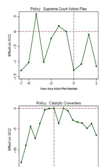
I. INTRODUCTION

There is a paucity of evidence about the efficacy of environmental regulation in developing

countries. However, this question is important for at least two reasons.1 First, "local" pollutant

concentrations are exceedingly high in many developing countries and they impose substantial

health costs, including shortened lives (Chen, Ebenstein, Greenstone, and Li 2011). Thus,

understanding the most efficient ways to reduce local pollution could significantly improve

wellbeing in developing countries. Second, the Copenhagen Accord makes it clear that it is up to

individual countries to devise and enforce the regulations necessary to achieve their national

commitments to combat global warming by reducing greenhouse gas emissions. Since most of

the growth in greenhouse gas (GHG) emissions is projected to occur in developing countries,

such as India and China, the planet's wellbeing rests on the ability of these countries to

successfully enact and enforce environmental regulations.

                                                     India provides a compelling setting to explore the efficacy of environmental regulations

in a developing country for several reasons. First, India's population of nearly 1.2 billion

accounts for about 17 percent of the planet's population. Second, the country is experiencing

rapid economic growth of about 6.4 percent annually over the last two decades, which is placing

significant pressure on the environment. For example, Figure 1, Panel A demonstrates that

ambient particulate matter concentrations in India are five times the level of concentrations in the

United States (while China's are seven times the U.S. level) in the most recent years with

comparable data, while Figure 1, Panel B shows that water pollution concentrations in India are


1
  There is a large literature measuring the impact of environmental regulations on air quality, with many of them
finding that significant regulation-induced reductions in pollution concentrations in the United States. See, for
example, Chay and Greenstone (2003 and 2005), Greenstone (2003), Greenstone (2004), Henderson (1996), Hanna
and Oliva (2010), and so forth. However, given the institutional differences that exist between the United States and
many developing countries, it is not clear that knowledge on what “works” in the United States is necessarily
relevant in other contexts.


                                                                                                                                                                                                                         2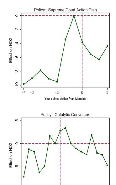
also higher. Third, India has a surprisingly rich history of environmental regulations that dates

back to the 1970s, providing a rare opportunity to answer these questions with extensive panel

data.2 Finally, India remains below the income levels at which the Environmental Kuznets curve

literature predicts that pollution concentrations turn downward (e.g., Grossman and Krueger,

1995; Shafik and Bandyopadhyay, 1992; Selden and Song, 1994; Stern and Common, 2001;

Copland and Taylor, 2004), implying that it is at a stage of development where economic growth

trumps environmental concerns. Consequently, taking the predictions of these models at face

value, it may be reasonable to expect that most of the environmental policies implemented to

date have been ineffective.

                This paper presents a systematic evaluation of India’s environmental regulations. The

analysis is conducted with a new city-level panel data file for the years 1986-2007 that we

constructed from data on air pollution, water pollution, environmental regulations, and infant

mortality in India. The air pollution data cover about 140 cities, while the water pollution data

comprises information from 424 cities (162 rivers).                                                                                  Neither the government nor other

researchers have ever assembled a city-level panel database of India's anti-pollution laws.

Furthermore, we are unaware of a comparable data set in any other developing country.

Additionally, we believe that this is the first paper to relate infant mortality rates to

environmental regulations in a developing country context.3

                We considered two key air pollution policies—the Supreme Court Action Plans and the

Mandated Catalytic Converters—that centered on stemming both industrial and vehicular


2
  Previous papers have compiled data sets for a cross-section of cities or a panel for one or two cities. A few notable
papers that focus on a particular city include: Foster and Kumar (2008; 2009), which examines the effect of CNG
policy in Delhi; Takeuchi, Cropper, and Bento (2007), which studies the impact of automobile policies in Mumbai;
Davis (2008), which looks at the effect of driving restrictions on air quality in Mexico; and Hanna and Oliva (2011),
which explores the effects of a refinery closure in Mexico City.
3
  See Chay and Greenstone (2003) for the relationship between infant mortality and the Clean Air Act in the United
States. Burgess, Deschenes, Donaldson, and Greenstone (2011) estimate the relationship between weather extremes
and infant mortality rates using the same infant mortality data used in this paper.


                                                                                                        3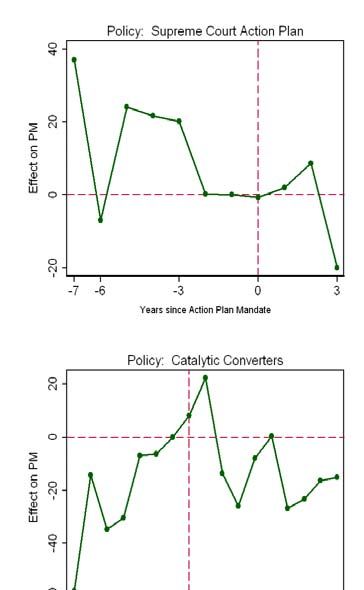
pollution.4 We also consider the primary water policy, the National River Conservation Plan,

which focused on reducing industrial pollution in the rivers and creating sewage treatment

facilities. These regulations resemble environmental legislation in the United States and Europe,

thereby providing an interesting study of the efficacy of similar regulations across very different

institutional settings.

                                                     The results are mixed: the air regulations have led to improvements in air pollution, while

the water pollution regulations have been ineffective. In the preferred econometric specification

which controls for city fixed effects, year fixed effects and pre-existing trends among adopting

cities, we find that the Supreme Court-mandated Action Plans are associated with declines in

NO2 concentrations; however, we do not observe an effect of the policy on SO2 or PM.

Additionally, the requirement that new automobiles have catalytic converters is associated with

economically large reductions in PM, SO2, and NO2 of 19 percent, 69 percent, and 15 percent,

respectively, five years after its implementation. In contrast, the National River Conservation

Plan, which is the cornerstone of water policy in India, had no impact on the three measures of

water quality we consider.

                                                     In light of these findings, we tested whether the catalytic converter policy was associated

with changes in measures of infant health. The data indicate that a city’s adoption of a policy is

associated with a decline in infant mortality, but this relationship is not statistically significant.

As we discuss below, there are several reasons to interpret the infant mortality results cautiously.

                                                     In sum, our findings shed light on two broader questions. First, the results suggest that

environmental policies can be effective in developing countries, even in cases where income

level falls within the range where the environmental Kuznets curve would predict that


4
 We also documented the implementation of other key anti-pollution efforts. However, these policies (such as the
Problem Area Action Plans, and the multiple sulfur requirements for fuel) had insufficient variation in their
implementation across cities and/or time to obtain reliable estimates.


                                                                                                                                                                                                                         4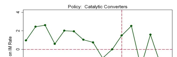
environmental quality should be decreasing.           Second, the results suggest that bottom-up

environmental policies are more likely to succeed than policies, like the water pollution

regulations that are initiated by political institutions.       Thus, while the results suggest that

developing countries are able to effectively curb pollution, regulations imposed by international

treaties, like those contemplated as part of an effort to confront climate, may have limited

success without widespread political support from within.


       The paper proceeds as follows. Section II provides a brief history of environmental

regulation in India and the policies under consideration, while Section III describes our data.

Section IV describes the trends in pollution in India. Section V describes our empirical methods,

and Section VI provides our results. Section VII discusses the results, and Section VIII

concludes.

II. BACKGROUND

India has a relatively extensive set of regulations designed to improve both air and water quality.

Its environmental policies have their roots in the Water Act of 1974 and Air Act of 1981. These

acts created the Central Pollution Control Board (CPCB) and the State Pollution Control Boards

(SPCBs), which are responsible for data collection and policy enforcement, and also developed

detailed procedures for environmental compliance. Following the implementation of these acts,

the CPCB and SPCBs quickly advanced a national environmental monitoring program

(responsible for the rich data underlying our analysis). The Ministry of Environment and Forests

(MoEF), created in its initial form in 1980, was established largely to set the overall policies that

the CPCB and SPCBs were to enforce (Hadden, 1987).


                                                5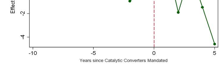
The Bhopal Disaster of 1984 represented a turning point in the course of Indian

environmental policy.                                                                                                                                                            The government’s treatment of victims of the Union Carbide plant

explosion “led to a re-evaluation of the environmental protection system,” with increased

participation of activist groups, public interest lawyers, and the judiciary in the environmental

space (Meagher 1990). The Supreme Court instigated a wide expansion of fundamental rights of

citizens and there was a steep rise in public interest litigation (Cha, 2005). These developments

led to some of India's first concrete environmental regulations, such as the closures of limestone

quarries and tanneries in Uttar Pradesh in 1985 and 1987, respectively.5

                                                     Throughout the 1980s and 1990s, India continued to adopt a series of policies designed to

counteract the effects of growing environmental damage. The analysis focuses on two key air

pollution policies, the Supreme Court Action Plans and the catalytic converter requirements, and

the primary water pollution policies, the National River Conservation Plan. These policies were

at the forefront of India’s environmental efforts. Importantly, these policies were also phased

into different cities in different years, providing the basis for this paper’s research design.

                                                     The first policy we focus on is the Supreme Court Action Plans. The Action Plans are

part of a broad, ongoing effort to stem the tide of rising pollution in cities identified by the

Supreme Court of India as critically polluted. Measured pollution concentrations are clearly a

key ingredient in the determination of these designations. In 1996, Delhi was the first city order

to develop an action plan, while the most recent action plans were mandated in 2003.6 To date,

17 cities have been given orders to develop action plans.


5
  See Rural Litigation and Entitlement Kendra v. State of Uttar Pradesh (Writ Petitions Nos. 8209 and 8821 of
1983), and M.C. Mehta v. Union of India (WP 3727/1985).
6
   As documented in the court orders, the Supreme Court ordered nine more action plans in critically polluted cities
“as per CPCB data” after Delhi. A year later, the Court chose four more cities based on their having pollution levels
at least as high as Delhi’s. Finally, a year later, nine more cities (some repeats) were identified based on Respired
SPM (smaller diameter) levels.


                                                                                                                                                                                                                         6
In light of the Supreme Court’s reputation as a driver of environmental reform in India, as
well as the overwhelming approval of Delhi’s CNG bus program as part of its action plan, many
believe that these policies have made significant gains in improving air quality. At least one
round of plans was directed at cities with unacceptable levels of Respired Suspended Particulate
Matter (RSPM), which is a subset of particulate matter (PM) that includes particles of especially
small size. Given the heavy focus on vehicular pollution, it is reasonable to presume that the
plans affected NO2 levels. Finally since SO2 is frequently a co-pollutant, it may be reasonable to
expect the Action Plans to affects its ambient concentrations.
We then examine a policy that mandated the use of catalytic converters. The fitment of
catalytic converters is a common means of reducing vehicular pollution across the world, due to
the low cost of its end-of-the-pipe technology. In 1995, the Supreme Court required that all new
petrol-fueled cars in the four major metros (Delhi, Mumbai, Kolkata, Chennai) were to be fitted
with converters. In 1998, the policy was extended to 45 other cities. It is plausible that this
regulation could affect all three of our air quality indicators; however, the prediction is strongest
for NO2.7
Finally, we study the cornerstone of efforts to improve water quality, the National River
Conservation Plan (NRCP). Begun in 1985 under the name Ganga Action Plan (Phase I), the
water pollution control program expanded first to tributaries of the Ganga River, including the
Yamuna, Damodar, and Gomti in 1993. It was later extended in 1995 to the other regulated
rivers under the new name of NRCP. Today, 164 cities on 34 rivers are covered by the NRCP.
The criteria for coverage by the NRCP are vague at best, but many documents on the plan cite
7
Public response to the catalytic converter policy was unfavorable for several reasons: petrol’s lower fuel share
made the scope of the policy somewhat narrower than, for example, the mandate for low-sulfur in diesel fuel;
unleaded fuel, which is known to be a prerequisite for smooth catalytic converter functioning, was at best
inconsistently available until 2000; and selective implementation in only certain cities of India caused leakage of
automobile purchases to other cities not covered by the policy.
7the CPCB Official Water Quality Criteria, which include standards for BOD, DO, FColi, and pH
measurements in surface water. Much of the focus has centered around domestic pollution
control initiatives over the years (Asian Development Bank, 2007).
The centerpiece of the plan has been and continues to be the Sewage Treatment Plant
(STP). The interception, diversion, and treatment of sewage through piping infrastructure and
treatment plant construction has been coupled with installation of community toilets, crematoria,
and public awareness campaigns to curtail domestic pollution. The NRCP has been panned in
the media for a variety of reasons, including poor cooperation among participating agencies,
imbalanced funding of sites, and inability to keep pace with the growth of sewage output in
India’s cities (Suresh et al, 2007, p. 2). If the policy is found to have had an effect, it may be
expected to be particularly visible in FColi levels, since this is the parameter most correlated
with domestic pollution in the data.
III. DATA
To conduct the analysis, we compiled the most comprehensive city-level panel data file ever
assembled on air pollution concentrations, water pollution concentrations, and environmental
policies in India. We supplemented this data file with a city-level panel data file on infant
mortality rates. This section provides details on each data source.
A. Air Pollution Data
This paper takes advantage of an extensive and growing network of environmental monitoring
stations across India. Starting in 1987, India’s Central Pollution Control Board (CPCB) began
compiling readings of Nitrogen Dioxide (NO2), Sulfur Dioxide (SO2), and particulate matter with
8diameter less than 100 µm (PM). The data were collected as a part of the National Air Quality
Monitoring Program (NAMP), a program established by the CPCB to help identify, assess, and
prioritize the pollution controls needs in different areas, as well as to help in identifying and
regulating potential hazards and pollution sources.8 Individual State Pollution Control Boards
(SPCBs) are responsible for collecting the pollution readings and sending the data to the CPCB
for checking, compilation, and analysis. The air quality data are from a combination of CPCB
online and print materials for the years 1987-2007.9
While the CPCB reports that there are currently 342 functional air quality monitoring
stations in 127 Indian cities, there has been much movement and reclassification of these
monitors over the years. In total, our full dataset includes 572 monitors in 140 cities. For some
cities, data is collected in certain, but not all, years.10 In 1987, the first year in our dataset, the
functioning monitors cover 20 cities, while 125 cities are monitored by 2007 (see Appendix
Table 1 for summary statistics of the data, by year). On average, there are 2.3 monitors per city,
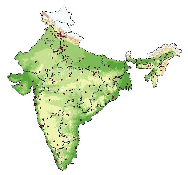
with 78 percent of cities including data from more than one monitor in a given year.11 Figure 2
maps the location of the cities with air pollution data in at least one year.
The three pollutants can be attributed to a variety of sources. PM is regarded by the
CPCB as a general indicator of pollution, receiving key contributions from “fossil fuel burning,
industrial processes and vehicular exhaust.” SO2 emissions, on the other hand, are
8
For a more detailed description of the data collection program, see http://www.cpcb.nic.in/air.php (accessed on
June 25, 2011).
9
From the CPCB, we obtained monthly pollution readings per city from 1987-2004, and yearly pollution readings
from 2005-2007. The monthly data were averaged to get annual measures.
10
The CPCB requires that 24 hour samplings be collected twice a week from each monitor for a total of 104
observations per monitor per year. As this goal is not always achieved, 16 or more successful hours of monitoring
are considered representative of a given day’s air quality, and 50 days of monitoring in a year are viewed as
sufficient for data analysis. In some cities, readings are conducted more frequently. For example, readings are
conducted daily in Delhi. This more frequent data is not included in our dataset.
11
Each monitor is classified as belonging to one of three types of areas: residential (71 percent), industrial (26
percent), or sensitive (2 percent). The rationale for specific locations of monitors is, unfortunately, not known to us
at this time so all monitors with sufficient readings are included in the analysis.
9predominantly a byproduct of thermal power generation; globally, 80 percent of sulfur emissions
in 1990 were attributable to fossil fuel use (Smith, Pitcher and Wigley, 2001). NO2 is viewed by
the CPCB as an indicator of vehicular pollution, though it is produced in almost all combustion
reactions.
B. Water Pollution Data
The CPCB also administers water quality monitoring, in cooperation with state pollution control
boards (SPCBs). As of 2008, 1,019 monitoring stations are maintained under the National Water
Monitoring Programme (NWMP), covering rivers and creeks, lakes and ponds, drains and
canals, and groundwater sources. We focus on rivers due to the consistent availability of data on
river quality, the seriousness of pollution problems along the rivers, and, most significantly, the
attention that rivers have received from public policy. We have obtained from the CPCB, in
electronic format, observations from 489 monitors in 424 cities along 162 rivers between the
years 1986 and 2005 (see Appendix Table 1).12 Figure 3 maps the location of the water quality
monitors on India’s major rivers.
The CPCB collects either monthly or quarterly river data on 28 measures of water
quality, of which nine are classified as “core parameters.” We focus on three of these core
parameters: Biochemical Oxygen Demand (BOD), Dissolved Oxygen (DO), and Fecal Coliforms
(FColi). We chose these measurements largely because of their presence in CPCB Official Water
Quality Criteria, and also their continual citation in planning, analysis, and commentary, as well
as the consistency of their reporting.13
12
From 1986 to 2004, monthly data is available. For 2005, the data is only available yearly.
13
See Water Quality: Criteria and Goals (February 2002); Status of Water Quality in India (April 2006); and the
official CPCB website, http://www.cpcb.nic.in/Water_Quality_Criteria.php.
10These indicators can be briefly summarized as follows. BOD is a commonly-used broad
indicator of water quality that measures the quantity of oxygen required by the decomposition of
organic waste in water. High values are indicative of heavy pollution; however, since water-
borne pollutants can be inorganic as well, BOD cannot be considered a comprehensive measure
of water purity. DO is similar to BOD except that it is inversely proportional to pollution; that is,
lower quantities of dissolved oxygen in water suggest greater pollution because water-borne
waste hinders mixing of water with the surrounding air, as well as hampering oxygen production
from aquatic plant photosynthesis. The third water parameter, FColi, is a count of the number of
coliform bacteria per 100 milliliters (ml) of water. While not directly harmful, these organisms
are associated with animal and human waste and are correlated with the presence of harmful
pathogens. FColi is thus considered to be an indicator of domestic pollution. It is measured as
the most probable number of fecal coliform bacteria per 100 milliliters (ml) of water. Since its
distribution is approximately ln normal, FColi is reported as ln(number of bacteria per 100 ml)
throughout the paper.
C. Regulation Data
India has implemented a variety of environmental initiatives over the last two decades. We have
assembled a dataset that systematically documents changes in policy at the city-year level for the
cities in the air and water pollution datasets. To the best of our knowledge, we believe that a
comparable data set has never been compiled.
The data were compiled from a variety of sources. We first collected and utilized print
and web documents from the Indian government, including the CPCB, the Department of Road
Transport and Highways, the Ministry of Environment and Forests, and several Indian SPCBs.
11Next, we used reports and data from secondary sources, including the World Bank, the Emission
Controls Manufacturers Association, and Urbanrail.net.
Table 1 summarizes the prevalence of these policies in the data file of city-level air and
water pollution concentrations by year. Columns (1a) and (2a) report the number of cities with
air and water readings, respectively. The remaining columns detail the number of these cities
where each of the studied policies is in force. The subsequent analysis exploits the variation in
the year of enactment of these policies across cities.14
D. Infant Mortality Rate Data
We obtained annual city-level infant mortality data from annual issues of Vital Statistics of India
for the years prior to 1996.15 In subsequent years, city level data are no longer available from a
central source; therefore, we visited the registrar’s office for each of India’s larger states and
collected the necessary documents directly.16 Many births and deaths are not registered in India
and the available evidence suggests that this problem is greater for deaths so the infant mortality
rate is likely downward biased. Although the infant mortality rate from the Vital Statistics data
is about a third of the rate measured from state-level survey measures of infant mortality rates
(i.e., the Sample Registration System), trends in the Vital Statistics and survey data are highly
correlated. Although these data are likely to be noisy, we are unaware of reasons to believe that
the measurement error is correlated with the pollution measures. Notably, Burgess et al. (2011)
find that they are correlated with inter-annual temperature variation.
14
Appendix Table 2 replicates Table 1 for all cities in India.
15
We digitized the city-level data from the books. All data were double entered and checked for consistency.
16
Specifically, we attempted to obtain data in all states except the Northeastern states (which have travel
restrictions) and Jammu-Kashmir. We were able to obtain data from Andhra Pradesh, Chandigarh, Delhi, Goa,
Gujarat, Himachal Pradesh, Karnataka, Kerala, Madhya Pradesh, Maharashtra, Punjab, Rajasthan, and West Bengal.
12E. Additional Variables
We collected city-level, socio-economic variables that are used as controls in the subsequent
analysis.17 First, we obtained district-level data on population and literacy rates from the 1981,
1991, and 2001 Census of India. For non-census years, we linearly interpolated these variables.
Second, we collected district-level expenditure per capita data, which is a proxy for income. The
data are imputed from the survey of household consumer expenditure carried out by India's
National Sample Survey Organization in the years 1987, 1993, and 1999 and are imputed in the
missing years.
IV. TRENDS IN POLLUTION CONCENTRATIONS AND INFANT HEALTH
A. Trends in Mean Pollution Levels over Time
Figure 4 provides a graphical representation of the trends in national air and water quality. Panel
A plots the average air quality measured across cities, by pollutant, from 1987 to 2007; Panel B
graphs water quality measured across city-rivers, by pollutant, from 1986 to 2005. Table 2
provides corresponding sample statistics. Specifically, it provides the average pollution levels
for the full sample, as well as values at the start and end of the sample timeframe.
Air pollution has fallen. As shown in Panel A, ambient PM concentrations fell quite
steadily over the sample timeframe, from 252.1 µg/m3 in 1987-1990 to 209.5 µg/m3 in 2004-
2007. This represents about a 17 percent reduction in PM. The SO2 trend line is flat until the
late 1990s, and then declines sharply. Comparing the 1987-1990 to 2004-2007 time periods,
mean SO2 decreased from 19.4 to 12.2 µg/m3 (or 37 percent). Finally, NO2 appears more
volatile over the start of the sample period, but then falls after its peak in 1997.
17
Consistent city-level data in India is notoriously difficult to obtain. We instead acquired district level data, and
matched cities to their respective districts.
13While air quality has generally improved over the past twenty years, the trends in water quality are more mixed. As seen in Panel B of Figure 4, BOD steadily worsens throughout the late 1980s and early 1990s but then begins to improve starting around 1997. The improvement, though, did not make up for early losses, as mean BOD worsens by about 19 percent from 3.47 to 4.14 mg/l over the sample period. FColi drops precipitously in the 1990s but rises somewhat in the 2000s. The general decrease in FColi is notable, as it suggests that domestic water pollution may be abating, in spite of the alarmingly fast-paced growth in sewage generation seen in India (Suresh et al, 2007). Over the sample period, the natural log of the number of fecal coliform bacteria per 100 ml declined from 6.41 to 5.28. DO declines fairly steadily over time (a fall in DO indicates worsening water quality) from 7.21 to 7.03 mg/l. B. Trends in Infant Health Infant mortality rates are an appealing measure of the effectiveness of environmental regulations, relative to measures of adult health. This is because it seems reasonable to presume that infant health will be more responsive to short and medium changes in pollution and the first year of life is an especially vulnerable one so losses of life expectancy may be large. Since 1987, infant mortality has fallen sharply in urban India (Panel C of Figure 4). As Panel C of Table 2 shows, the infant mortality rate fell from 29.6 per 1000 live births in 1987-1990 to 16.7 in 2001-2004. C. A More Disaggregated Analysis Is there spatial variation in these trends? To explore this, we next graph the distributions of air and water quality across cities at the start and end of the sample period. Specifically, we provide kernel density estimates of air pollutant distributions across Indian cities for 1987-1990 and 14
2004-2007 in Figure 5A, and similar estimates of water pollutant distributions for 1986-1989 and

2002-2005 in Figure 5B. We then construct similar graphs for infant mortality in Figure 5C.

                                                     Figure 5A shows that not only have the means of PM and SO2 decreased, but their entire

distributions have shifted to the left over the last two decades. The 10th percentiles of PM and

SO2 pollution both declined by about 10 percent from 1987-1990 to 2004-2007. Particularly

striking, however, is the drop in the 90th percentile of ambient SO2 concentration: 38.2 to 23.0

µg/m3, or about 40 percent. Consistent with trends in Figure 2, the distribution of NO2 across

cities does not appear to change much over the sample time frame. In fact, if anything, the

distribution of pollution appears to have worsened, with the 10th percentile rising from 8.5 to

10.4 µg/m3 and the 90th percentile rising from 42.6 to 47.0 µg/m3.

                                                     The changes in the distribution of water quality are more variable over time (Figure 5B).

The distribution of BOD has widened over the last twenty years, with many relatively higher

readings of BOD in the later time period.18 While the 10th percentile of BOD has dropped

slightly, the 90th percentile has increased from 5.78 to 7.85 mg/l between the earlier and more

recent periods. In contrast, the FColi distribution has largely shifted to the left. The relatively

clean cities show tremendous drops in FColi levels, with the 10th percentile value falling from

3.61 to 1.79, while dirtier cities show more modest declines. Lastly, the DO distribution does not

appear to have changed noticeably, with very little difference between the graphs of the earlier

and later periods.

                                                     Figure 5C reveals a marked improvement in infant mortality rates over this period.

Indeed, the kernel density graphs reveal a leftward shift in the distribution of infant mortality

rates.


18
 The right tail of the 2002-2005 period extends to 100 mg/l. In the figure, it has been truncated at 20 to give a
more detailed picture of the distribution.


                                                                                                                                                                                                                         15
V. ECONOMETRIC APPROACH
This section describes a two-stage econometric approach for assessing whether India’s
regulatory policies impacted air and water pollution concentrations. The first-stage is an event
study-style equation:
1 !!" = ! + !! !!,!" + !! + !! + β!!" + !!"
!
where Yct is one of the six measures of pollution in city c in year t. The city fixed effects, !! ,
control for all permanent unobserved determinants of pollution across cities, while the inclusion
of the year fixed effects, µt, non-parametrically adjust for national trends in pollution, which is
important in light of the time patterns observed in Figure 2. The equation also includes controls
for per capita consumption and literacy rates (X) in order to adjust for differential rates of growth
across districts. To account for differences in precision due to city size, the estimating equation
is weighted by the district-urban population.19
The vector Dτ,ct is composed of a separate indicator variable for each of the years before
and after a policy is in force. τ is normalized so that it is equal to zero in the year the relevant
policy is enacted; it ranges from -17 (for 17 years before a policy's adoption in a city) through 12
(for 12 years after its adoption). All τ's are set equal to zero for non-adopting cities; these
observations aid in the identification of the year effects and the β's. In the air pollution
regressions, there are separate Dτ,ct vectors for the Supreme Court Action Plan and catalytic
converter policies, so each policy's impact is conditioned on the other policy's impact.20
19
City-level population figures are not systematically available, so we use population in the urban part of the district
in which the city is located to proxy for city-level population.
20
The results are qualitatively similar in terms of sign, magnitude, and significance from models that evaluate each
policy separately.
16The sample for equation (1) is based on the availability of data for a particular pollutant
in a city. For adopting cities, a city is included in the sample if it has at least one observation
three years or more before the policy's enactment and four or more years afterward. If a city
does not have any post-adoption observations or did not enact the relevant policy, then that city
is required to have at least two observations for inclusion in the sample.
The parameters of interest are the στ's, which measure the average annual pollution
concentration in the years before and after a policy's implementation. These estimates are
purged of any permanent differences in pollution concentrations across cities and of national
trends due to the inclusion of the city and year fixed effects. The variation in the timing of the
adoption of the individual policies across cities allows for the separate identification of the στ's
and the year fixed effects.
In the below, the estimated στ's are plotted against the τ's. These event study graphs
provide an opportunity to visually assess whether the policies are associated with changes in
pollution concentrations. Additionally, they allow for an examination of whether pollution
concentrations in adopting cities were on differential trends. These figures will inform the
choice of the preferred second-stage model.
The second-stage of the econometric approach formally tests whether the policies are
associated with pollution reductions with three different specifications. In the first, we fit the
following equation:
2a !! = !! + !! 1(!"#$%&)! + !!
where 1(!!"#$%)! is an indicator variable for whether the policy is in force (i.e., τ ≥ 1). Thus, π1
tests for a mean shift in pollution concentrations after the policy's implementation.
17In several cases, the event study figures reveal trends in pollution concentrations that
predate the policy's implementation (even after adjustment for the city and year fixed effects).
Therefore, we also fit the following equation:
2b !! = !! + !! 1(!"#$%&)! + !! τ+!! .
This specification includes a control for a linear time trend in event time, τ, to adjust for
differential pre-existing trends in adopting cities.
Equations (2a) and (2b) test for a mean shift in pollution concentrations after the policy's
implementation. A mean shift may be appropriate for some of the policies that we evaluate. On
the other hand, the full impact of some of the policies may emerge over time as the government
builds the necessary institutions to enforce a policy and as firms and individuals begin to take the
steps necessary to comply with them. For example, an evolving policy impact seems possible
for the Supreme Court Action Plans since they specify actions that polluters must take over
several years.
To allow for a policy's impact to evolve over time, we also report the results from fitting:
2c !! = !! + !! 1(!"#$%&)! + !! τ + !! (1(!"#$%&)! ×τ) + !! .
From this specification, we report the impact of a policy 5 years after it has been in force as
!! + 5!! .
There are three remaining estimation issues about equations (2a) through (2c) that bear
noting. First, the sample is chosen so that there is sufficient precision to compare the pre- and
post-adoption periods. Specifically, for two of the policies it is restricted to values of τ for which
there are at least twenty city by year observations to identify the στ's. For the catalytic converter
regressions, the sample therefore covers τ = -7 through τ = 9 and for the National River
Conservation Plan regressions it includes τ = -7 through τ = 10 (see Appendix Table 3). In the
18case of the Supreme Court action plan policies which were implemented more narrowly, the
sample is restricted to values of τ for which there are a minimum of 15 and this leads to a sample
that includes τ = -7 through τ = 3. Second, the standard errors for these second stage equations
are heteroskedastic consistent. Third, the equation is weighted by the inverse of the standard
error associated with the relevant στ to account for differences in precision in the estimation of
these parameters.
VI. RESULTS
A. Air Pollution
Figure 6 presents the event study graphs of the impact of the policies on PM (Panel A), SO2
(Panel B), and NO2 (Panel C). Each graph plots the estimated στ's from equation (1). The year
of the policy's adoption, τ = 0, is demarcated by a vertical dashed line in all figures.
Additionally, pollution concentrations are normalized so that they are equal to zero in τ = -1, and
this is noted with the dashed horizontal line.
These figures are "hands above the table" summaries of the data in the sense that they
visually report all the data that underlie the subsequent regressions. It is evident that accounting
for differential trends in adopting cities is crucial, because the parallel trends assumption of the
simple difference in differences or means shift model (i.e., equation (2a)) is violated in many
cases. This is particularly true in the case of the catalytic converter policies which were
implemented in cities where pollution concentrations were worsening. This upward pre-trend in
pollution concentrations is also apparent in the case of the Supreme Court Action Plans (SCAPs)
and NO2. In these instances, equations (2b) and (2c) are more likely to produce valid estimates
of the policies’ impacts. With respect to inferring the impact of the policies, the figures suggest
19that the catalytic converter policy was effective at reversing the trend toward increasing pollution
concentrations.
To test these results more formally, Table 3 reports regression results from the estimation
of separate equations for each pollutant and policy pair. For each pollutant-policy pair, the first
column reports the estimate of π1 from equation (2a), which tests whether στ is on average lower
after the implementation of the policy. The second column reports the estimate of π1 and π2 from
the fitting of equation (2b) in the second column for each pollutant. Here, π1 tests for a policy
impact after adjustment for the trend in pollution levels (π2). The third column reports the results
from equation (2c) that allows for a mean shift and trend break after the policy’s implementation.
It also reports the estimated effect of the policy five years after implementation for the policies,
which is equal to !! + 5!! .
Reading across Panel A, it is evident that the SCAPs have a mixed record of success.21
There is little evidence of an impact on PM or SO2 concentrations. The available evidence for an
impact comes from the NO2 regressions that control for pre-existing trends. In column (8) the
estimated impact would not be judged statistically significant, while in column (9) it is of a large
magnitude and would be judged marginally significant.
In contrast, the regressions confirm the visual impression that the catalytic converter
policies were strongly associated with air pollution reductions. In light of the differential pre-
trends in pollution in adopting cities and that the policy's impact will only emerge as the stock of
cars changes, the richest specification (equation (2c)) is likely to be the most reliable. It
indicates that 5 years after the policy was in force, PM, SO2, and NO2 declined by 48.6 µg/m3,
13.4 µg/m3, and 4.5 µg/m3, respectively. The PM and SO2 declines are statistically significant
21
Note that for the Supreme Court Action Plans, the analysis lags the policies by one year. The dates we have
correspond to Court Orders, which mandated submission of Action Plans. However, the Plans were frequently
reviewed by a special committee and only afterwards declared/implemented.
20when judged by conventional criteria, while the NO2 decline is not. These declines are 19
percent, 69 percent, and 15 percent of the 1987-1990 nationwide mean concentrations,
respectively. These percentage declines are large and this reflects the rapid rates at which
ambient pollution concentrations were increasing before the implementation of the catalytic
converter policy in adopting cities-- put another way, if the pre-trends had continued then
pollution concentrations would have reached levels much higher than those recorded in the 1987-
1990 period.22
B. Effects of Policies on Water Quality
Figure 7 presents event study analyses of the impact of the National River Conservation Plan
(NRCP) on BOD (Panel A), ln(FColi) (Panel B), and DO (Panel C). As in Figure 6, the figures
plot the results from the estimation of equation (1). From the figures, there is little evidence that
the NRCP was effective at reducing pollution concentrations.
Table 4 provides the corresponding regression analysis and is structured similarly to
Table 3. The evidence in favor of a policy impact is weak. BOD concentrations are lower after
22
There is a tradeoff to in including a greater or smaller number of event years or taus in the second-stage analysis.
The inclusion of a wider range of taus provides a larger sample size, allows for more precise estimation of pre and
post adoption trends. But, at the same time, it moves further away from the event in question so that other
unobserved factors may confound the estimation of the policy effects. Further, it exacerbates the problems
associated with estimating the taus from an unbalanced panel data file of cities. In contrast, including fewer taus
would result in a smaller sample size (and number of cities) to estimate pre and post trends, but it the analysis would
be more narrowly focused around the policy event. Appendix Table 3 reports on the number of city by year
observations that identify the στ's associated with each event year.
We investigated the sensitivity of the results to the number of taus included in the analysis. Specifically, we
estimated models that include a wider range of taus (between [-14,4] for the SCAPs and [-9,9] for the Catalytic
Converters), as well as models that limit the taus to a narrower range (between [-4,4] for the SCAPs and [-5,5] for
the Catalytic Converters), The application of these alternative samples to the preferred specification, equation (2c),
produces results that are qualitatively similar to those in Tables 3 and 4. The SCAP is associated with a large and
significant decline in NO2 with the narrower range. With the wider range, the SCAP continues to be associated with
a decline in NO2 but it no longer would be judged to be statistically significant; however, it is associated with a
statistically significant decline in PM. The pattern of the coefficients for the Catalytic Converters policy is similar to
that of Table 3, regardless of increasing or decreasing the range of taus.
21the implementation of NRCP, but the decline occurs several years prior to the implementation of
the plan (Panel A). While NRCP targets domestic pollution, the data fail to reveal an
improvement in FColi concentrations (Panel B), which is the best measure of domestic sourced
water pollution. The results from the fitting of equation (2c) are reported in column (9) and
confirm the perverse visual impression that the NRCP is associated with a worsening in DO
concentrations (recall, lower DO levels indicate higher pollution concentrations).23
The finding that the NRCP has not been successful is not surprising in light of some
supplementary research into process outcomes. For example, as of March, 2009, 152 out of 165
towns officially covered under NRCP have been approved for Sewage Treatment Plant (STP)
capacity building, but only 82 of those towns have actually built any capacity. Additionally, as
of March, 2009, there has not been any spending of federal or state monies on the NRCP in
fifteen NRCP towns (National River Conservation Directorate, 2009). Furthermore, the Centre
for Science and Environment (CSE) in New Delhi calculates that the 2006 treatment capacity
was only 18.5 percent of the full sewage burden (Suresh et al, 2007, p. 11).
C. Effects of Catalytic Converters on Infant Mortality
The catalytic converter policy is the most strongly related to improvements in air pollution. This
subsection explores whether this policy is associated with improvements in human health, as
measured by infant mortality rates. Specifically, we fit equation (1) and equations (2a) - (2c),
where the infant mortality rate, rather than pollution concentration, is the outcome of interest.
We note several aspects of this estimation. First, despite a large data collection exercise
to obtain the infant mortality data (including going to each state capital to obtain additional
23
This finding that the NRCP had little impact on the available measures of water pollution is unchanged by
increasing or decreasing the number of event years or taus (i.e., changing the event years to include [-9,12] or to
include [-5,5]) in the second-stage analysis.
22registry data), there are fewer cities in the sample.24 Second, the dependent variable is
constructed as the ratio of infant deaths to births, so we weight equation (1) by the number of
births in the city that year. Third, it is natural to be interested in using the catalytic converter
induced variation to estimate the separate impacts of each of the three forms of air pollution on
infant mortality in a two-stage least squares setting. However, such an approach is invalid in this
setting because, even in the best case where the exclusion restriction is valid, there is a single
instrument for three endogenous variables. Fourth, the infant mortality rate data do not provide
any characteristics of the parents or other covariates, so it is not possible to determine the degree
to which the results are due to shifts in the composition of parents that alter the observed infant
population's health endowment. This issue is a greater challenge in light of the possibly
substantial underreporting of infant births and deaths in these data.
Figure 8 and Table 5 report the results. In light of the differential pre-existing trend, the
column (3) specification is likely to be the most reliable. It suggests that the catalytic converter
policy is associated with a reduction in the infant mortality rate of 0.86 per 1,000 live births.
However, this estimate is imprecise and is not statistically significant.
VII. DISCUSSION
This paper's analysis is related to at least two key economics questions. First, is there a
deterministic relationship between income and environmental quality? Second, why are some
environmental policies so much more effective than others? The paper's results shed new light
on these questions.
24
When the air pollution sample is restricted to the sample used to estimate the infant mortality equations, the
catalytic converter policy is associated with substantial reductions in PM and SO2 concentrations but not of NO2
concentrations.
23A. Contradicting Predictions from the Environmental Kuznets Curve Literature
The Environmental Kuznets Curve (EKC) predicts greater environmental degradation as income
rises for countries at low incomes levels (Grossman and Krueger, 1995; Bandypadhyay, 1992).
When income levels rise beyond a high enough point, individuals will no longer be willing to
trade off environment quality for economic growth and resources will be available to invest in
enforcing environmental regulation. At this point, economic growth will be correlated with
environmental improvements.
The range for the turning point varies considerably across empirical studies. For
example, Grossman and Kruger (1995) estimate the turning point for SO2 at around $4,000, with
the turning point for most pollutants around or below $8,000. Similarly, Shafik and
Bandyopadhyay’s (1992) study (which was used in the 1992 World Development Report)
estimated turning points of about $3,000 to $4,000 for local air pollutant concentrations. Using
an updated data set, but following Grossman and Kruger’s econometric specification, Harbaugh,
Levinson, and Wilson (2002) find higher turning points (e.g., for SO2 the turning points range
from $13,000 to $20,000), but the results are not robust to changes in the specification.
Similarly, they find high and varying turning points for PM, ranging from $2,000 to $13,000,
depending on the specification.
Two of this paper's results contradict the EKC model. First, India’s per capita GDP was
$374 in 1990 when environment regulations became salient there and this is substantially below
the estimated turning point.25 However, this paper demonstrates that that the catalytic converter
mandate was associated with substantial improvements in air quality.
Second, the EKC model predicts similar trends for local pollutants. However, there are
substantial differences in trends across the various types of air and water pollution. Moreover,
25
India’s GDP was obtained from the World Development Indicators.
24You can also read