GUV long-term measurements of total ozone column and effective cloud transmittance at three Norwegian sites
←
→
Page content transcription
If your browser does not render page correctly, please read the page content below

Atmos. Chem. Phys., 21, 7881–7899, 2021
https://doi.org/10.5194/acp-21-7881-2021
© Author(s) 2021. This work is distributed under
the Creative Commons Attribution 4.0 License.

GUV long-term measurements of total ozone column and
effective cloud transmittance at three Norwegian sites
Tove M. Svendby1 , Bjørn Johnsen2 , Arve Kylling1 , Arne Dahlback3 , Germar H. Bernhard4 , Georg H. Hansen1 ,
Boyan Petkov5,6 , and Vito Vitale6
1 NILU  – Norwegian Institute for Air Research, Kjeller, Norway
2 Norwegian  Radiation and Nuclear Safety Authority, Østerås, Norway
3 Department of Physics, University of Oslo, Oslo, Norway
4 Biospherical Instruments Inc., San Diego, CA, USA
5 Department of Psychological Sciences, Health and Territory, D’Annunzio University, Chieti, Italy
6 National Research Council, Institute of Polar Sciences (CNR-ISP), Bologna, Italy

Correspondence: Tove M. Svendby (tms@nilu.no)

Received: 20 January 2021 – Discussion started: 5 February 2021
Revised: 18 April 2021 – Accepted: 21 April 2021 – Published: 25 May 2021

Abstract. Measurements of total ozone column and effec-          transmittance in Ny-Ålesund indicate that there has been a
tive cloud transmittance have been performed since 1995 at       significant change in albedo during the past 25 years, most
the three Norwegian sites Oslo/Kjeller, Andøya/Tromsø, and       likely resulting from increased temperatures and Arctic ice
in Ny-Ålesund (Svalbard). These sites are a subset of nine       melt in the area surrounding Svalbard.
stations included in the Norwegian UV monitoring network,
which uses ground-based ultraviolet (GUV) multi-filter in-
struments and is operated by the Norwegian Radiation and
Nuclear Safety Authority (DSA) and the Norwegian Institute       1   Introduction
for Air Research (NILU). The network includes unique data
sets of high-time-resolution measurements that can be used       The amount of stratospheric ozone decreased significantly
for a broad range of atmospheric and biological exposure         both globally and over Norway during the 1980s and 1990s
studies. Comparison of the 25-year records of GUV (global        (WMO, 2018; Svendby and Dahlback, 2004). This decrease
sky) total ozone measurements with Brewer direct sun (DS)        was mainly caused by the release of ozone-depleting sub-
measurements shows that the GUV instruments provide valu-        stances (ODSs). In 1987, the Montreal Protocol was signed
able supplements to the more standardized ground-based in-       with the aim of phasing out the production of ODSs. Mo-
struments. The GUV instruments can fill in missing data and      tivated by this treaty, the Norwegian Environment Agency
extend the measuring season at sites with reduced staff and/or   established the programme “Monitoring of the atmospheric
characterized by harsh environmental conditions, such as         ozone layer” in 1990. Five years later, in 1995/1996, the net-
Ny-Ålesund. Also, a harmonized GUV can easily be moved           work was expanded and “the Norwegian UV network” was
to more remote/unmanned locations and provide independent        established with funding from the Norwegian Ministry of
total ozone column data sets. The GUV instrument in Ny-          Health and Care Services and the Norwegian Environment
Ålesund captured well the exceptionally large Arctic ozone       Agency. This network consists of nine ground-based ultra-
depletion in March/April 2020, whereas the GUV instrument        violet (GUV) radiometers located at sites between 58 and
in Oslo recorded a mini ozone hole in December 2019 with         79◦ N (Fig. 1). The network has been in operation for 25
total ozone values below 200 DU. For all the three Norwe-        years, and the measurements are undertaken by the Norwe-
gian stations there is a slight increase in total ozone from     gian Radiation and Nuclear Safety Authority (DSA; formerly
1995 until today. Measurements of GUV effective cloud            the Norwegian Radiation Protection Authority, NRPA) and
                                                                 the Norwegian Institute for Air Research (NILU). The GUV

Published by Copernicus Publications on behalf of the European Geosciences Union.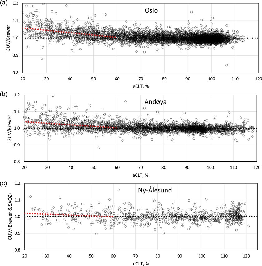
7882        T. M. Svendby et al.: GUV long-term measurements of total ozone column and effective cloud transmittance

                                                                         strated to be a good alternative to expensive spectroradiome-
                                                                         ters (Dahlback, 1996; Bernhard et al., 2005; Sztipanov et al.,
                                                                         2020).
                                                                            In this study, we present a 25-year time series of total
                                                                         ozone column (TOC) from the Norwegian UV Network. We
                                                                         have focused on three stations operated by NILU located
                                                                         in Oslo/Kjeller, at Andøya/Tromsø, and in Ny-Ålesund as
                                                                         shown by red circles in Fig. 1. All stations are equipped
                                                                         with additional total ozone measuring instruments such as
                                                                         Brewer spectrophotometers and a Système d’Analyse par
                                                                         Observation Zénithale (SAOZ) instrument. TOCs derived
                                                                         from the GUV instruments are compared to measurements
                                                                         from other ground-based instruments. In addition, they are
                                                                         compared with satellite retrieved data sets. The current work
                                                                         also presents observed changes in total ozone and effective
                                                                         cloud transmittances.

                                                                         2     Material and methods

                                                                         2.1    Instruments in the Norwegian UV network

Figure 1. The Norwegian UV network. Grey circles represent sta-          The GUV is a multi-wavelength filter radiometer manufac-
tions operated by DSA, whereas red circles represent sites operated      tured by Biospherical Instruments Inc. (BSI), San Diego
by NILU. The large red circle to the south includes the three stations   (Bernhard et al., 2005). The detector unit is environmentally
at Østerås (DSA), Blindern, in Oslo, and Kjeller. The instrument in      sealed and temperature stabilized, facilitating long-term re-
Tromsø (blue circle) was moved to Andøya in 2000.                        liable operation under harsh outdoor conditions. The GUV
                                                                         instruments have five channels in the UV range where each
                                                                         channel has a dedicated filter, a photodetector, and electron-
instruments allow the calculation of the UV index, retrievals            ics that sample the output at a rate of about 3 Hz. The chan-
of total ozone column, cloud transmittance, and several other            nels measure simultaneously global (direct and diffuse) solar
UV-related dose products (Dahlback, 1996; Høiskar et al.,                irradiance at several UV wavelengths, which can be used to
2003; Bernhard et al., 2005). Data and dose products have                reconstruct the solar spectrum in the UV range and to com-
been used in several international studies (Bernhard et al.,             pute biological doses, the UV index, total ozone, and cloud
2013, 2015, 2020; Schmalwieser et al., 2017; Lakkala et al.,             transmittance.
2020), and the data are available at https://github.com/uvnrpa              The UV network consists of 12 multiband filter radiome-
(last access: 19 May 2021) and Johnsen et al. (2020).                    ters (model GUV-541 and GUV-511) (Bernhard et al., 2005).
   The spectral distribution of solar UV radiation reaching              Nine of them are continuously operating at the network loca-
the ground depends on the optical properties of the atmo-                tions (Table 1) and three serve calibration purposes and are
sphere, the solar zenith angle (SZA), and reflection from                backups in case of failure at some of the stations. The instru-
the Earth’s surface. The transmission of solar radiation in              ment in Oslo/Kjeller is a GUV-511, whereas the instruments
the UVB region (280–315 nm) through the stratosphere is                  at the other sites are GUV-541. Both instrument types have
primarily determined by the amount of stratospheric ozone,               four channels in the UV region (centre wavelengths 305,
whereas the attenuation in the troposphere is mainly due to              320, 340, and 380 nm). In addition, GUV-541 has a fifth UV
scattering by air molecules (Rayleigh scattering), aerosols,             channel at 313 nm, whereas GUV-511 has a fifth channel for
and clouds. Generally, a decrease in total ozone column leads            measuring photosynthetically active radiation (PAR: 400–
to an increase in UVB radiation, assuming no changes in                  700 nm). The bandwidths of the UV channels are ∼ 10 nm
cloudiness or other UV-affecting parameters.                             (full width at half maximum, FWHM). All instruments are
   High-wavelength-resolution spectroradiometers can pro-                temperature stabilized at 40 ◦ C. Measurements are recorded
vide detailed information about the spectral distribution of             as 1 min averages, and for each instrument/site this represents
UV radiation. Stamnes et al. (1991) showed that spectra from             several million records since the start in 1995.
such instruments can be used to determine total ozone and                   The GUV-511 in Oslo was purchased already in 1993 and
cloud transmission accurately. However, simpler and cheaper              was installed at the University of Oslo (UiO) to test the in-
radiometers with channels in both the UVB and the UVA re-                strument performance and to develop appropriate software.
gions, such as the GUV instruments, have also been demon-                In July 2019, this instrument was moved to Kjeller (∼ 18 km

Atmos. Chem. Phys., 21, 7881–7899, 2021                                                   https://doi.org/10.5194/acp-21-7881-2021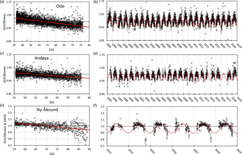
T. M. Svendby et al.: GUV long-term measurements of total ozone column and effective cloud transmittance                                                            7883

Table 1. Overview of the locations, instrument types, and institutes involved in the Norwegian UV network.

    Site                                       Location            GUV type (serial)                  Supporting                                      Responsible
                                                                                                      TOC                                             institute
                                                                                                      instruments
    Landvik                                58.0◦ N, 08.5◦ E        GUV-541                                                                            DSA
    Blindern, Oslo (1994–2019)             59.9◦ N, 10.7◦ E        GUV-511                            Brewer no. 42                                   NILU/UiO
    Kjeller1 (2019 →)                      60.0◦ N, 11.0◦ E        GUV-511                            Brewer no. 42                                   NILU
    Østerås                                60.0◦ N, 10.6◦ E        GUV-541, GUVis-35112                                                               DSA
    Bergen                                 60.4◦ N, 05.3◦ E        GUV-541                                                                            DSA
    Finse                                  60.6◦ N, 07.5◦ E        GUV-541                                                                            DSA
    Kise                                   60.8◦ N, 10.8◦ E        GUV-541                                                                            DSA
    Trondheim                              63.4◦ N, 10.4◦ E        GUV-541                                                                            DSA
    Andøya (2000 →)                        69.3◦ N, 16.0◦ E        GUV-541                            Brewer no. 104                                  NILU3
    Tromsø4 (1995–1999)                    69.7◦ N, 17.0◦ E        GUV-541                            Brewer no. 104                                  NILU
    Ny-Ålesund                             78.9◦ N, 11.9◦ E        GUV-541                            Brewer no. 505,7 , SAOZ, Pandora6               NILU7
  1 GUV and Brewer no. 42 were moved from Blindern (University of Oslo) to Kjeller in June 2019. 2 GUVis-3511 was installed in 2018. 3 The instrument is inspected daily
  by staff at Alomar, Andøya Space Center. 4 GUV and Brewer no. 104 were moved from Tromsø to Andøya in the winter of 1999/2000. 5 Brewer no. 50 is operated by
  ISAC-CNR, Italy. 6 Pandora measurements started in spring 2020. 7 The instrument is inspected daily by staff from the Norwegian Polar institute.

east of UiO) due to termination of total ozone/UV activity at                           the DS method cannot be used. Measurements of the Brewer
the University of Oslo. Similarly, to assure continuation of                            global irradiance (GI) are an alternative to the ZS method
the GUV time series, the instrument in Tromsø was moved                                 and are also based on the principle of measuring scattered
to the Arctic Lidar Observatory for Middle Atmosphere Re-                               UV radiation from the sky.
search (ALOMAR) facility at Andøya in 2000, about 130 km                                   The Norwegian Brewer instruments have been calibrated
southwest of Tromsø. Initial studies showed that the ozone                              by the International Ozone Service (IOS, Canada) every
climatology is very similar at the two sites (Høiskar et al.,                           year since installation in the 1990s, except from the sum-
2001); however, the UV level is normally slightly higher at                             mer of 2020 when the calibration was prohibited under the
Andøya as the site is located ∼ 50 km south of Tromsø.                                  COVID-19 restrictions. These frequent calibrations are done
   With a few minor exceptions, the GUV instruments have                                to ensure high-quality Brewer measurements and to make
been running continuously since 1995. The GUV instrument                                sure that the instruments are well maintained and perform
at Andøya has been subjected to some problems, most likely                              DS measurements within an accuracy of ±1 %. The instru-
caused by an event of water intrusion. In spring 2013 an er-                            ment B42 in Oslo is an MKV single-monochromator Brewer,
ror with the 380 nm channel was discovered and the instru-                              which might be influenced by stray light (Karppinen et al.,
ment was sent to BSI for repair. Two years later, in 2015,                              2015). Therefore, in this study we have only used Brewer DS
the 320 nm channel failed and had to be replaced. During                                data with ozone slant column below 1100 DU where the ef-
these time periods spare GUV instruments were deployed                                  fect of stray light is negligible. All Brewer DS daily mean
from the DSA.                                                                           data from Oslo/Kjeller and Andøya are available at the World
   As listed in Table 1 there are three Brewer spectrome-                               Ozone and Ultraviolet Radiation Data Centre (WOUDC,
ters in operation in Norway: one in Oslo/Kjeller (B42), one                             https://woudc.org/, last access: 19 May 2021). Also, the Ital-
in Tromsø/Andøya (B104), and one in Ny-Ålesund (B50).                                   ian Brewer (B50) in Ny-Ålesund has been calibrated regu-
Generally, the Brewer instruments have been approved by                                 larly by IOS Canada, last time in 2018, which showed that
the WMO as reliable high-quality instruments (WMO, 2018;                                the instrument has been stable since the previous calibration
Fioletov et al., 2008). The direct sun (DS) algorithm is the                            in 2015. However, there are limited Brewer DS measure-
primary measurement mode of the Brewer and is based                                     ments available in Ny-Ålesund, and the measuring season
on measurements of the intensity of direct sunlight at five                             is relatively short due to the high latitude (79◦ N). Thus, in
wavelengths between 306 and 320 nm. The precision of this                               addition to Brewer DS data we have used SAOZ measure-
method can be as high as 0.15 % (Scarnato et al., 2010), but                            ments to obtain quality-assured ozone data from the early
the absolute accuracy relies on an appropriate calibration.                             spring and fall. SAOZ derives total ozone from the Chap-
Under cloudy conditions, total ozone can be derived by mea-                             puis bands in the visible part of the spectrum through the
suring the intensity of scattered radiation from the zenith. As                         differential optical absorption spectroscopy (DOAS) method
shown by Stamnes et al. (1990) there are some limitations                               (Pommereau and Goutail, 1988), and contrary to Brewer
of the zenith sky (ZS) method, but nevertheless this method                             it can only measure ozone when the solar beam pathway
provides useful information about total ozone content when                              through the atmosphere is large (solar zenith angle > 85◦ ),

https://doi.org/10.5194/acp-21-7881-2021                                                                       Atmos. Chem. Phys., 21, 7881–7899, 2021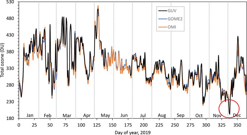
7884         T. M. Svendby et al.: GUV long-term measurements of total ozone column and effective cloud transmittance

i.e. around sunrise and sunset. Analyses and QC of the SAOZ      where ki is a constant (response factor), Ri0 (λ) is the rela-
data are performed at LATMOS (France) in the framework           tive spectral response function for channel i, and F (λ) is the
of the SAOZ global network (http://saoz.obs.uvsq.fr/index.       spectral irradiance at wavelength λ. During the calibration,
html, last access: 19 May 2021). In this study, we have used     the Sun is used as the light source, and the irradiance F (λ)
SAOZ daily average total ozone on days where both sunrise        is measured by a reference radiometer at the same time as
and sunset measurements are available. The data are stored       the co-located GUV is recording the voltage Vi . The rel-
in the Network for the Detection of Atmospheric Compo-           ative spectral response functions for the GUV instruments
sition Change (NDACC) database (http://www.ndaccdemo.            were characterized at the optical laboratory of the Norwegian
org/, last access: 19 May 2021). Based on experience and re-     Radiation and Nuclear Safety Authority (DSA). When Vi ,
sults from intercomparison campaigns, the SAOZ total ozone       Ri0 (λ), and F (λ) are known, one can calculate the constant ki
uncertainty is estimated to be within 3 % (Hendrick et al.,      and the absolute response for channel i: Ri (λ) = ki Ri0 (λ).
2011).                                                               The shape of the solar UV spectrum at the Earth’s surface
   The GUV data in the present study have been compared          depends mostly on the solar zenith angle (SZA) and the TOC.
to OMI/Aura and GOME-2/MetOp-A TM3DAM v4.1 total                 Thus, the spectral distribution of Ri0 (λ)F (λ) in Eq. (1) will
ozone data from Oslo, Andøya, and Ny-Ålesund. The satel-         depend on these parameters (Dahlback, 1996). The error in
lite data from OMI and GOME-2 are available from 2004            the derived irradiance depends on how much the atmospheric
and 2007, respectively. These data are assimilated prod-         conditions at the time of the measurement differ from those
ucts, based on the TM3DAM software developed by Royal            at the time of the absolute calibration. This is discussed in
Netherlands Meteorological Institute, KNMI (Eskes et al.,        more detail in Sect. 2.3.
2003). The GOME-2 and OMI assimilated TOC values                     The calibration procedure described above is normally
are publicly available and are provided on a daily basis         done during large national or international intercomparison
via ESA’s TEMIS project (http://www.temis.nl, last access:       campaigns, where the GUV instruments are operating syn-
19 May 2021). The data files include error estimates, which      chronously with co-located high-resolution reference spec-
are dependent on location and time of year. During winter,       troradiometers. One of these campaigns was arranged in Oslo
the error can be as high as 8 %–10 %, whereas the error esti-    in 2005, initiated through the national project Factors Affect-
mates usually are around 1 %–2 % during summer.                  ing UV Radiation in Norway (FARIN) (Johnsen et al., 2008;
   In Sect. 4.3, trends in effective cloud transmittance from    WMO, 2008). Here the GUV instruments were intercom-
the GUV instruments are discussed, and cloud data from           pared with a Bentham spectroradiometer belonging to DSA,
the Norwegian Centre for Climate Services (NCCS; https:          which is closely linked to the Quality Assurance of Spec-
//klimaservicesenter.no, last access: 19 May 2021) are be-       tral Ultraviolet Measurements in Europe (QASUME) world
ing used to help in the interpretation of these measure-         travelling reference spectroradiometer. Another large inter-
ments. These data describe the number of clear-sky days ob-      comparison campaign, which included the QASUME ref-
served every month. Cloud observations are performed three       erence spectroradiometer, was arranged in May/June 2019
times per day, but we have selected the measurements at          (PMOD/WRC, 2019).
12:00 UTC to reflect the period where GUV noontime val-              A key factor for the maintenance of a homogenous and
ues are measured. The data describe the fraction of clouds as    stable calibration scale for the network instruments is a sys-
a number (NN) ranging from 0 to 8. NN = 0 means clear sky,       tem for quality control which accounts for long-term changes
whereas NN = 8 means completely overcast. In our study we        in the absolute response factors ki . In Norway, this is imple-
have classified the day as “clear” if NN at 12:00 UTC has the    mented via a dedicated travelling reference GUV-541, which
value of 0, 1, or 2. NN = 2 means that a quarter of the sky is   has been transported to the respective stations every sum-
covered by clouds.                                               mer since 1995. The travelling instrument is set up next to
                                                                 the stationary GUV, and synchronous measurements with the
2.2    Calibrations                                              two instruments are performed for about 1 week. The irradi-
                                                                 ances from the two collocated instruments are compared to
The procedure for calibrating the GUV instruments is de-         results from the 2005 calibration campaign, where the drift
scribed by Dahlback (1996) and only briefly presented below.     for all instruments and channels was set to unity. Relative to
When the GUV Teflon diffuser is illuminated by a source,         this 2005 calibration, yearly drift factors di for the individual
the photodetector transforms the radiation to an electric cur-   channels (and instruments) are derived. These drift factors
rent which subsequently is converted to a voltage signal. The    are used to modify the response factor in Eq. (1), ki0 = ki /di .
measured voltage of channel i is                                 If di changes from one year to the next, a linear change in di is
       Z∞                                                        assumed for periods between the two intercomparisons. The
                            ∞
                            X                                    method is described in more detail in WMO (2008). DSA
Vi = ki Ri0 (λ)F (λ)dλ ≈ ki   Ri0 (λ)F (λ)1λ,              (1)
                              λ=0
                                                                 is responsible for these annual assessments of drift and de-
         0                                                       termination of correction factors. Assessments of long-term
                                                                 drift diR for the travelling reference GUV itself are made at

Atmos. Chem. Phys., 21, 7881–7899, 2021                                            https://doi.org/10.5194/acp-21-7881-2021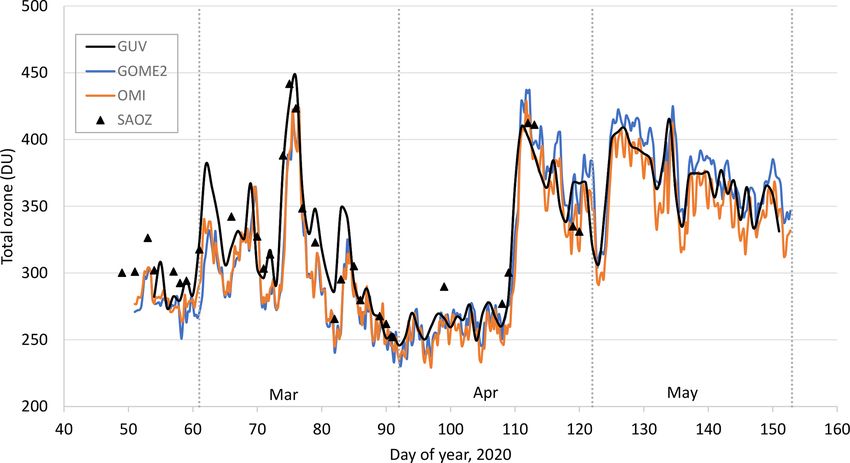
T. M. Svendby et al.: GUV long-term measurements of total ozone column and effective cloud transmittance                    7885

the optical laboratory at DSA. Additionally, the travelling        Anderson et al., 1987). The choice of ozone profile in the cal-
reference GUV has been shipped to the manufacturer every 1         culations of N -value lookup tables is especially important for
or 2 years since 1996 for an independent evaluation of long-       the winter when the SZA is large. Lapeta et al. (2000) found
term drift and for technical services.                             that an inappropriate ozone profile may cause uncertainties
                                                                   up to 10 % in the retrieved TOC for SZA > 75◦ . Sensitivity
2.3   Retrievals of total ozone and effective cloud                studies from Dahlback (1996) showed that the errors in total
      transmittance                                                ozone, related to an inappropriate atmospheric profile in the
                                                                   RTM, were less than 1 % for SZA < 65◦ . However, the error
The GUV data products described in this work consist of            could be as large as 30 % (at SZA = 80◦ ) if a subarctic winter
measurements used in combination with a radiative trans-           profile was replaced with a tropical atmospheric profile. This
fer model (RTM) based on the discrete ordinate method              latter example represents an extreme situation in Norway.
(Stamnes et al., 1988; Dahlback and Stamnes, 1991). When              To quantify the effects of clouds, aerosols, and changing
solar radiation passes through the atmosphere, a portion of        surface albedo, a cloud transmission factor is introduced. It
the UVB radiation will be absorbed by ozone. Other fractions       is defined as the measured irradiance at wavelength chan-
of the radiation will be multiple scattered or absorbed by air     nel i and solar zenith angle SZA, Fi (SZA), compared to the
molecules, aerosols, and clouds (Stamnes et al., 2017). The        modelled irradiance at a cloudless and aerosol-free sky with
total ozone column (TOC) is determined from the GUV in-            a none-reflecting surface, Fic (SZA). Fic is calculated for the
struments by comparing a measured and calculated N value,          same wavelength and solar zenith angle as the actual mea-
where the calculated N value is derived from the radiative         surement Fi , and a channel insensitive to ozone absorption
transfer model. The N value is defined as the ratio of irradi-     is selected. The estimates of cloud transmission and opti-
ances in two different UV channels, with spectral response         cal depth are sensitive to ground reflection, implying that an
functions Ri (λ) and Rj (λ). One of the channels is sensitive      accurate determination of cloud attenuation requires precise
to total ozone, whereas the other one is significantly less sen-   knowledge of the surface albedo. Stamnes et al. (1991) intro-
sitive. Hence, the N value is defined as                           duced the term effective cloud transmittance to account for
                   ∞
                                                                   the influence of surface albedo and aerosols on cloud atten-
                                                                   uation. The effective cloud transmittance (eCLT) is defined
                   P
                         Ri (λ)F (λ, SZA, TOC)1λ
                   λ=0                                  Vi         as
N(SZA, TOC) =       ∞                               =      , (2)
                   P                                    Vj
                         Rj (λ)F (λ, SZA, TOC)1λ                                         Fi (SZA)
                   λ=0                                             eCLT(SZA) = 100                 .                          (3)
                                                                                         Fic (SZA)
where F (λ,SZA, TOC) is the solar spectral irradiance at
                                                                   In this study, the 340 nm channel has been selected to de-
wavelength λ, solar zenith angle SZA, and TOC. Vi and
                                                                   termine the eCLT. Alternatively, the 380 nm channel can be
Vj are the measured voltages in channel i and j , respectively.
                                                                   used, but the derived eCLT is virtually independent of the
In this study the ratio channel(320 nm) / channel(305 nm) is
                                                                   choice of the 340 or 380 nm channel. For both wavelengths,
used for measuring and modelling the N values in Eq. (2).
                                                                   the incoming solar radiation is insensitive to ozone, meaning
Prior to the measurements, the RTM was used to create a
                                                                   that the eCLT is only sensitive to clouds, aerosols, and the
lookup table of N for all relevant combinations of SZA and
                                                                   surface albedo. The eCLT may be larger than 100 % due to
TOC, and the GUV TOC is inferred by comparing the mea-
                                                                   multiple scattering of the solar radiation when broken clouds
sured Vi /Vj and modelled N values at the given SZA. The
                                                                   are present and the sun remains unobscured. Furthermore,
N tables calculated from the RTM are for clear skies, but the
                                                                   the presence of snow on the ground enhances the albedo and
table can also be applied to cloudy skies because the effect
                                                                   contributes to an additional multiple scattering. We do not at-
of clouds on spectral irradiance at 305 and 320 nm is quite
                                                                   tempt to separate the effects of clouds, aerosols, and albedo
similar compared to the large effect of ozone (Stamnes et al.,
                                                                   here, and the eCLT quantifies the combined influence of the
1991).
                                                                   three factors.
   The N tables described above are based on the
320/305 nm wavelength ratio and RTM calculations with
the TOMS V7 ozone climatology (McPeters et al., 1996),             3     Data analysis
which describes an idealized altitude profile of temperature,
pressure, and ozone. Previous studies have shown that N ta-        3.1    Harmonization of total ozone
bles generated from this atmospheric profile agreed well with
ozone values provided by the Dobson spectrophotometer              As described in Sect. 2.3, each GUV instrument has a unique
in Oslo during wintertime (Dahlback, 1996). Several other          set of N tables, and to obtain optimal ozone measurements
N tables are created for the GUV instruments, both for other       it is possible to switch between various tables depending on
wavelength ratios (e.g. 320/313 and 340/305 nm) and for            season and solar zenith angle. However, in our study we have
subarctic summer and subarctic winter profiles (defined by         only used one N table for a given station (with TOMS V7

https://doi.org/10.5194/acp-21-7881-2021                                            Atmos. Chem. Phys., 21, 7881–7899, 2021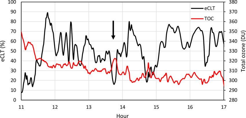
7886        T. M. Svendby et al.: GUV long-term measurements of total ozone column and effective cloud transmittance

Figure 2. Ratios of GUV / Brewer(DS) ozone values measured in Oslo (a, b), Tromsø/Andøya (c, d), and in Ny-Ålesund (e, f). SAOZ ozone
data are also used in Ny-Ålesund. Panels (a), (c), and (e) show TOC ratios as a function of SZA, where the red lines represent the linear fit.
Panels (b), (d), and (f) show daily TOC ratios for all years with simultaneous measurements. The statistical fit functions are marked as red
curves.

ozone climatology (McPeters et al., 1996) and 320/305 nm                 struments have been stable and homogenous since the start
channel ratio) to simplify the ozone estimates and avoid arte-           in 1995.
facts in trends and statistics generated by lookup table (N ta-             As seen from Fig. 2 there is a clear seasonality in the
ble) changes. To account for possible seasonal errors in total           TOC ratio. This can both be attributed to an instrumen-
ozone related to the above-mentioned inaccuracies in the at-             tal SZA dependence and/or a seasonal variability related to
mospheric profile and variations in surface albedo (snow/ice             the atmospheric profile in the RTM and N tables used for
on the ground), we have homogenized the GUV measure-                     ozone retrievals. Inspections of GUV minute values per-
ments with respect to Brewer direct sun (DS) total ozone                 formed throughout a day do not necessarily give a very
measurements. All Brewer DS data are daily mean values,                  clear explanation of the variability. Figure 3 shows two ex-
identical to the data available at the WOUDC database.                   amples from April and June 2018, where GUV TOCs in
   Figure 2 shows the GUV / Brewer DS ratio for the pe-                  Ny-Ålesund, normalized to noontime TOC (TOC_noon), are
riod 1995–2018 for days with available GUV and Brewer DS                 plotted throughout the day. The plot from April (Fig. 3, top
(and SAOZ) data. The GUV daily average total ozone val-                  panel) does not indicate any obvious SZA dependence in the
ues are calculated as 1 h averages around local noon, and                measurements. However, there is a significant spread in the
to limit possible errors caused by clouds, we have selected              ratio as SZA exceeds 82◦ , mainly due to noise in measure-
days where the noontime average eCLT from GUV is larger                  ments of the 305 nm channel. This might mask a possible
than 60 %. Also, GUV noontime TOC with standard devi-                    SZA dependence. Also, springtime ozone has normally large
ation larger than 20 DU have been flagged as “uncertain”                 day-to-day variations, and the morning TOC will often dif-
and are not included in the data analysis. Comparisons be-               fer from the evening value. Contrary to the upper panel, the
tween GUV (global sky) and Brewer DS time series in Fig. 2               bottom panel in Fig. 3 (from June 2018) indicates a clear
demonstrate highly consistent results; i.e. the individual in-           decrease in TOCs as SZA increases. At SZA = 78◦ , which

Atmos. Chem. Phys., 21, 7881–7899, 2021                                                     https://doi.org/10.5194/acp-21-7881-2021
T. M. Svendby et al.: GUV long-term measurements of total ozone column and effective cloud transmittance                            7887

                                                                       Figure 4. Total ozone and eCLT during 1 d (9 September 2018) with
                                                                       heavy clouds at Blindern, University of Oslo. Black arrow indicates
                                                                       a time where eCLT drops below 20 %.

                                                                       UV network (presented in Table 1 and Fig. 1), but for these
                                                                       instruments a different approach is used. A description of the
                                                                       method and results will be presented in a separate paper.
Figure 3. GUV TOC from Ny-Ålesund measured throughout two
selected periods: April 2018 (a) and June 2018 (b).                    3.2   Ozone cloud correction

Table 2. Results from statistical fit of GUV / Brewer(and SAOZ)        Under heavy cloud conditions the ozone retrievals are usually
ratio: a is the slope and b is the constant in Eq. (4). The standard   less accurate. An extreme example is discussed by Mayer et
deviation (SD) of the coefficients is included.                        al. (1998) for a thunderstorm case. They found that multiple
                                                                       scattering caused errors as large as 300 DU. A less extreme
  Station                            a ± SD          b ± SD            situation, which is more representative for Norway, is exem-
                                                                       plified in Fig. 4. The figure shows eCLT (black line) and total
  Oslo                −0.00154 ± 4 × 10⁻⁵       1.0814 ± 0.0018
                                                                       ozone column (red line) derived from GUV measurements in
  Andøya/Tromsø       −0.00119 ± 4 × 10⁻⁵       1.0642 ± 0.0025
                                                                       Oslo between 11:00 and 17:00 UTC on 9 September 2018.
  Ny-Ålesund            −0.0031 ± ×10−4         1.2129 ± 0.0112
                                                                       Figure 4 indicates a gradual ozone decrease throughout the
                                                                       day, but what is most interesting is the occurrence of ozone
                                                                       peaks when eCLT is very low. The uncertainty in total ozone
is the maximum SZA at midnight in Ny-Ålesund in June,                  increases as the cloud optical depth becomes very large, and
the average ratio TOC / TOC_noon is 0.97. For calculations             normally we use a cut-off at eCLT = 20 % and do not accept
of the harmonized noontime TOC it is of minor importance               ozone retrievals under these heavy cloud conditions.
whether the ozone values are corrected from a SZA or day-                 The example in Fig. 4 shows that total ozone increases by
of-year statistical fit function, but based on inspections of a        15 DU (∼ 5 %) when eCLT drops from 50 % to 16 % (see
number of daily minute values (such as Fig. 3, lower panel)            arrow in Fig. 4). However, the eCLT effect on ozone is less
a SZA correction is considered to give the best physical in-           evident for thinner clouds. In order to examine the impact
terpretation of the annual TOC variability.                            of clouds on TOC more systematically, we analysed the dif-
   When all measurements and seasons are considered as a               ference between SZA-corrected GUV noontime TOC and
whole, we have chosen an SZA correction of GUV TOC                     Brewer DS (and SAOZ) values as a function of eCLT, us-
data to harmonize with other ground-based instruments at the           ing data starting in 1995. Brewer DS measurements are not
stations. All available GUV / Brewer DS (and SAOZ) ratios              performed during cloudy conditions, so these measurements
have been fitted by the linear functions f (SZA) indicated by          are typically done during a clear period on the same day as
a red line in the left panels of Fig. 2:                               GUV recorded clouds around noon. The results for Oslo,
                                                                       Andøya, and Ny-Ålesund are shown in Fig. 5 for observa-
f (SZA) = a · SZA + b.                                          (4)
                                                                       tions with SZA < 80◦ . The figure shows that the ozone ratios
Here a and b are constants listed in Table 2 for the individ-          are characterized by gradual decreases for eCLT ranging be-
ual stations. The SZA-corrected total ozone value (TOC0 ) is           tween 20 % and 60 %, while for eCLT > 60 % the ratios vary
computed as TOC0 = TOC/f (SZA).                                        around one.
   The harmonization method described above is applied to                 Based on this analysis we have introduced a linear ozone
the three GUV instruments operated by NILU, which are                  correction g(eCLT) for eCLT < 60 %,
co-located with other ground-based ozone monitoring instru-            g(eCLT) = α · eCLT + β,                                        (5)
ments. Total ozone is also derived for the other stations in the

https://doi.org/10.5194/acp-21-7881-2021                                                 Atmos. Chem. Phys., 21, 7881–7899, 2021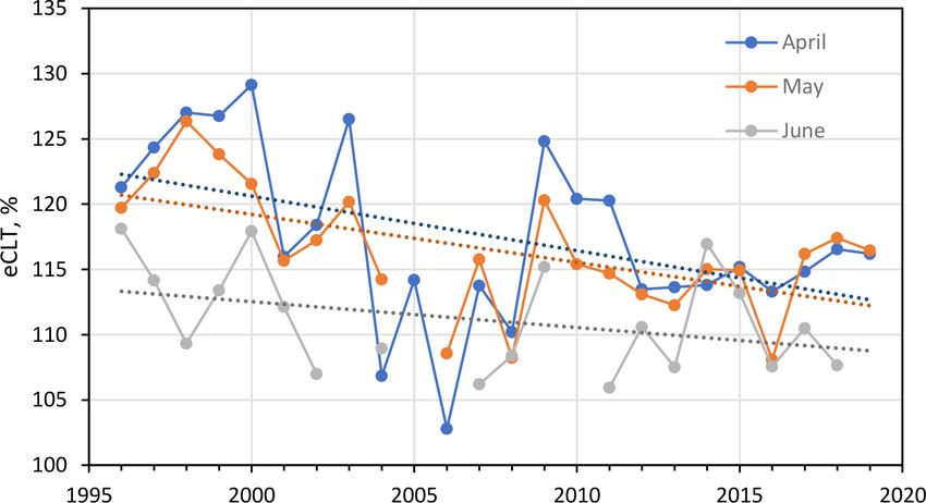
7888         T. M. Svendby et al.: GUV long-term measurements of total ozone column and effective cloud transmittance

Figure 5. Ozone difference between GUV and Brewer DS (and SAOZ) as a function of eCLT: Oslo (a), Andøya (b), and Ny-Ålesund (c).
The red dotted lines indicate the linear best fitting for eCLT < 60 %. The presence of eCLT higher than 100 % is discussed in Sect. 2.3.

Table 3. Ozone cloud correction for eCLT < 60 %, where α is the          The full GUV TOC time series from 1995 and onwards
slope and β is the constant in Eq. (5). The standard deviation (SD)   have been harmonized with respect to the SZA and eCLT
of the coefficients is included.                                      corrections described above. Specifically, TOCs have been
                                                                      divided by the fit function f (SZA) in Eq. (4). For cloudy
   Station                   α ± SD                β ± SD             conditions with effective cloud transmittance less than 60 %
   Oslo               −0.00137 ± 0.00011       1.0822 ± 0.0050        an additional correction g(eCLT), given in Eq. (5), has been
   Andøya/Tromsø      −0.00093 ± 0.00015       1.0558 ± 0.0068        applied to the data. With this harmonization, accurate GUV
   Ny-Ålesund         −0.00050 ± 0.00040       1.0300 ± 0.0185        total ozone values can be retrieved under most conditions.
                                                                      Table 4 gives an overview of correlation, bias, and standard
                                                                      deviation between GUV and Brewer DS (and SAOZ) for the
where α represents the slope and β is a constant. The values          original GUV data sets, shown in Fig. 2, and for the final cor-
of α and β for Oslo, Andøya, and Ny-Ålesund are summa-                rected data sets. As expected, the correlation increases and
rized in Table 3. For Ny-Ålesund there are few Brewer DS              the standard deviation (SD) is reduced after the GUV har-
and SAOZ data available on days with heavy clouds, and                monization. The biases for the final data sets are all within
consequently the eCLT correction function is more uncer-              ±0.3 %. The SD of the GUV–Brewer (and SAOZ) differ-
tain than the one for Oslo and Andøya. This is also reflected         ence is 2.5 %, 2.4 %, and 4.5 % for the Oslo, Andøya, and
from the high standard deviation of α in Table 3. The overall         Ny-Ålesund time series, respectively. This is a reduction of
eCLT correction for Ny-Ålesund is relatively small, i.e. a 2 %        0.5 %–1.1 % compared to SD for the uncorrected data sets.
correction when eCLT drops from 100 % to 20 %. The corre-                The ratios between GUV and Brewer DS (and SAOZ)
sponding ozone corrections for Oslo and Andøya are ∼ 5 %              TOC are visualized in Fig. 6 for the three stations: Oslo
and ∼ 4 %, respectively.                                              (top), Andøya (centre), and Ny-Ålesund (bottom). Compared

Atmos. Chem. Phys., 21, 7881–7899, 2021                                                  https://doi.org/10.5194/acp-21-7881-2021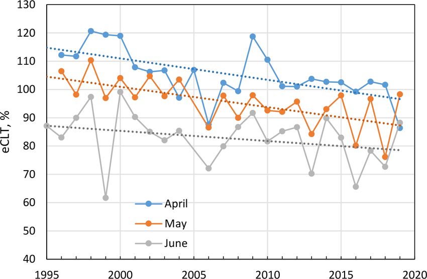
T. M. Svendby et al.: GUV long-term measurements of total ozone column and effective cloud transmittance                          7889

Table 4. Correlation, bias, and SD in total ozone from GUV and Brewer (and SAOZ) instruments. The left columns are for uncorrected GUV
data, whereas the right columns are for SZA- and CLT-corrected GUV total ozone data. Bias and SD are both expressed in DU and percent
(in parenthesis).

                                                Uncorrected                                       Corrected
                   Station        Correlation      Bias,          SD,             Correlation           Bias,        SD,
                                                  DU (%)       DU (%)                                 DU (%)      DU (%)
                   Oslo              0.969        2.9 (0.9)   12.0 (3.6)             0.984         −0.1 (0.0)     8.5 (2.5)
                   Andøya            0.983        0.1 (0.0)    9.9 (2.9)             0.989        −0.3 (−0.1)     8.4 (2.4)
                   Ny-Ålesund        0.966        0.8 (0.2)   17.8 (5.1)             0.976           0.9 (0.3)   15.7 (4.5)

Figure 6. Ratios of GUV / (Brewer and SAOZ) ozone values measured in Oslo (a), Tromsø/Andøya (b), and Ny-Ålesund (c) for the GUV
corrected data sets. Measurements for all SZA and eCLT values are included.

to Fig. 2 no systematic seasonality can be seen in the ratios.             4     Results
Ny-Ålesund is possibly an exception, where low GUV TOC
values are seen in late fall most of the years. These mea-                 4.1    Comparison with total ozone column from satellites
surements are performed at very high SZA (84–89◦ ) where
the GUV uncertainty is high. If we only consider GUV mea-
surements with SZA < 82◦ the high / low ratios in fall and                 Corrected GUV TOCs have been compared to GOME-2A
spring disappear and the standard deviation between GUV                    and OMI TM3DAM v4.1 (Eskes et al., 2003) data for Oslo,
and Brewer (and SAOZ) is reduced to 3.5 %.                                 Andøya, and Ny-Ålesund. It should be emphasized that
                                                                           GUV data are homogenized with respect to Brewer DS (and

https://doi.org/10.5194/acp-21-7881-2021                                                        Atmos. Chem. Phys., 21, 7881–7899, 2021
7890 T. M. Svendby et al.: GUV long-term measurements of total ozone column and effective cloud transmittance
Figure 7. Total ozone differences (in %) between GUV and GOME-2 (a, c, e) and GUV–OMI (b, d, f): Oslo (a, b), Andøya (c, d), and
Ny-Ålesund (e, f).
SAOZ) data and that any offset between Brewer and satellite Figure 7 and Table 5 show that GOME-2 gives slightly
data most likely will be reflected by offset in GUV–GOME-2 better agreement with GUV TOC compared to OMI. For
and GUV–OMI ozone data. Figure 7 shows the difference all stations, the SD is higher for GUV–OMI than for GUV–
(in %) of daily noontime GUV and GOME-2 total ozone GOME-2, both when the entire GUV time series and data
for the period 2007–2019 (left column) and GUV vs. OMI with SZA < 80◦ are considered. The standard deviations of
for the period 2004–2019 (right column). Results for Oslo the GUV–GOME-2 differences range from 3 %–6 % when
are shown in the top row, Andøya in the centre row, and all measurements are included but are reduced to ∼ 3 % if
Ny-Ålesund in the bottom row. The correlations, biases, and we only consider measurements with SZA < 80◦ . For GUV–
SDs are listed in Table 5. At Oslo, the noontime total ozone is OMI the corresponding SDs are in the range 4 %–9 % if
never calculated at SZA > 83◦ , which is the noontime SZA at all measurements are included and 3 %–4 % if data with
the winter solstice. As seen from the figure, the spread in the SZA < 80◦ are used. The overall biases between GUV and
GUV–GOME-2 difference increases as SZA exceeds 82◦ , es- satellite data are within ±1 % for all stations, but on average
pecially for Andøya. The statistics presented in Table 5 also OMI is slightly lower than GOME-2, especially at the two
indicate that the overall SD for Andøya is larger than for the northernmost stations.
other locations. The reason for this is not entirely clear but
can partially be attributed to a combination of uncertainties 4.2 Long-term changes in total ozone
in GUV and satellite measurements at this coastal area where
clouds, albedo, and topography vary on a small scale. For ex- For total ozone assessment and trends studies, the established
ample, drifting clouds at Andøya occur frequently and lead Brewer instruments would normally be used. However, as
to a large variability in the ratio of satellite and ground-based demonstrated in previous sections, GUV measurements can
UVI measurements during spring and summer when albedo provide realistic and stable time series and are suitable for
is low (Bernhard et al., 2013). Further, clouds represent an separate studies of long-term changes of the ozone layer.
atmospheric factor that can significantly reduce the accuracy GUV instruments that are co-located with a Brewer or an-
of both ground-based measurements and satellite TOC data other standard TOC instrument for 2–3 years (until harmo-
(Antón and Loyola, 2011). nization parameters are established) can afterwards be moved
to a new location for independent TOC measurements. The
Atmos. Chem. Phys., 21, 7881–7899, 2021 https://doi.org/10.5194/acp-21-7881-2021T. M. Svendby et al.: GUV long-term measurements of total ozone column and effective cloud transmittance 7891
Table 5. Correlation, bias, and SD in daily noontime total ozone from (a) GUV vs. GOME-2 for 2007–2019 and (b) GUV vs. OMI for
2004–2019. Bias and SD are both expressed in DU and percent (in parenthesis).
All SZA SZA < 80◦
Station Correlation Bias, ST, Correlation Bias, SD,
DU (%) DU (%) DU (%) DU (%)
(a) GUV vs. GOME-2
Oslo 0.974 2.2 (0.6) 11.2 (3.4) 0.979 2.4 (0.7) 10.1 (3.0)
Andøya 0.954 −1.3 (−0.4) 19.7 (5.8) 0.983 1.0 (0.3) 11.0 (3.3)
Ny-Ålesund 0.966 0.2 (0.1) 17.7 (5.1) 0.986 0.0 (0.0) 9.6 (2.8)
(b) GUV vs. OMI
Oslo 0.968 1.7 (0.5) 12.9 (3.9) 0.977 2.8 (0.8) 10.8 (3.2)
Andøya 0.904 2.0 (0.6) 28.9 (8.6) 0.972 2.2 (0.6) 14.0 (4.1)
Ny-Ålesund 0.963 2.8 (0.8) 18.2 (5.3) 0.984 3.8 (1.1) 10.5 (3.1)
harmonization procedure is used to minimize small system- The GUV network was established during a period where
atic errors in GUV TOC data and assumes that Brewer data a significant downward trend in total ozone had been ob-
are without error. However, it should be noted that TOC re- served for most places on Earth. Statistical analysis of the
trievals at large SZAs can be uncertain if the new site has Dobson (D56) time series from Oslo 1978–1998 revealed
a very different ozone climatology compared to the origi- an annual average total ozone decrease of −5.2 ± 0.6 % per
nal site, as explained in Sect. 2.3. Data from the GUV in- decade during this period (Svendby and Dahlback, 2002).
struments are also very useful to extend the measuring sea- For the Norwegian stations, a minimum in annual aver-
son at sites with reduced staff and/or characterized by harsh age total ozone was measured during the period 1993–1997
environmental conditions. The case of Ny-Ålesund, where (Svendby et al., 2020). Thus, a study of the trend in GUV
Brewer data are very sparse due to a rough climate that re- total ozone should also consider a possible influence by the
quires a high attendance, is a clear example of GUV useful- low values the first few years.
ness. In Ny-Ålesund as much as 52 % of TOC daily means Linear trends in the annual average total ozone at the three
have solely been based on GUV measurements during the stations have been calculated, and the results are shown in
last 5 years. Fig. 8: Oslo in the top panel, Andøya in the centre panel,
Even at sites like Oslo and Andøya, where good atten- and Ny-Ålesund in the bottom panel. For the Oslo station
dance and less harsh conditions allow more robust Brewer we have a full year of data in 1995, whereas the measure-
operations, GUV TOC can fill in missing data and extend the ments in Tromsø (Andøya) and Ny-Ålesund started in mid-
measuring season. Brewer zenith sky (ZS) or global irradi- 1995, and a full year of data is not available until 1996.
ance (GI) measurements (WOUDC, 2019) are normally per- Thus 1995 is omitted from the time series at these two sta-
formed under cloudy conditions. However, these measure- tions. Results from the linear regression analyses are pre-
ments can also be impacted by high SZA, heavy clouds, or sented in Table 6. In addition to changes in annual mean
technical problems. The last 5 years, 14 % of the daily mean total ozone, the table includes also linear trends for winter
TOC values at Andøya are retrieved from GUV to fill in for (December–February), spring (March–May), summer (June–
missing Brewer DS/ZS/GI measurements. August), and fall (September–November).
The overall GUV data coverage at the Norwegian stations The annual means in Oslo are based on data from January
is very good. If we disregard the two calibration campaigns to December, for Andøya the means are calculated for the
in 2005 and 2019, the GUV-511 in Oslo has been in op- months from February to mid-November, and data from Ny-
eration ∼ 99 % of all days since the start in 1995. Missing Ålesund are based on data from March to October. For the
days are mainly caused by power failure or minor technical two northernmost stations the winter averages cannot be re-
computer issues. TOC retrievals are performed on ∼ 95 % trieved because of the polar night. Note also that the fall trend
of all days, where the missing retrievals usually are related to results for Ny-Ålesund, presented in Table 6, do not include
heavy cloud conditions (eCLT < 20 %) with high uncertainty. November.
Due to the long and continuous GUV time series, trend anal- Due to different months included in the Oslo, Andøya,
yses based on these data will give a very good picture of the and Ny-Ålesund annual means, the absolute values are not
development of the ozone layer above Norway after 1995, comparable. Still, there are many similarities in the three
along a very wide latitudinal range. data sets. Even though Oslo and Ny-Ålesund are separated
by more than 2000 km, the years with low annual average
https://doi.org/10.5194/acp-21-7881-2021 Atmos. Chem. Phys., 21, 7881–7899, 20217892 T. M. Svendby et al.: GUV long-term measurements of total ozone column and effective cloud transmittance
Table 6. Seasonal and annual changes in total ozone in Oslo, at Andøya, and in Ny-Ålesund for the period (a) 1995–2019 (start year 1996
for Andøya and Ny-Ålesund) and (b) 1999–2019. Uncertainty is expressed as 2 · SD (2σ ). Results that are statistically significant are marked
in bold.
Winter Spring Summer Fall Annual
(a) TOC observational change, % per decade 1995/1996–2019
Oslo 2.92 ± 3.23 1.68 ± 2.27 0.97 ± 1.27 3.38 ± 1.50 2.33 ± 1.46
Andøya 1.30 ± 2.59 0.77 ± 1.37 2.95 ± 2.82 1.62 ± 2.22
Ny-Ålesund 3.84 ± 3.45 0.96 ± 1.28 2.02 ± 4.50 2.46 ± 2.15
(b) TOC observational change, % per decade 1999–2019
Oslo 1.75 ± 4.01 0.61 ± 2.85 0.68 ± 1.04 3.23 ± 2.01 1.54 ± 1.79
Andøya −0.39 ± 2.76 0.88 ± 1.50 3.00 ± 3.69 0.51 ± 2.60
Ny-Ålesund 1.39 ± 3.55 0.80 ± 1.56 1.52 ± 5.76 1.21 ± 2.42
TOC often coincide. Annual variations in the ozone trans-
port from its source region in the tropics toward the polar
regions during the winter will often have similar impacts at
all our stations, and variations in the Quasi-Biennial Oscilla-
tion (QBO), El Niño–Southern Oscillation (ENSO), the so-
lar cycle, and stratospheric aerosols will give significant in-
terannual variability in total ozone (WMO, 2018; Svendby
and Dahlback, 2004). The explanatory variables mentioned
above are often used in TOC trend studies to eliminate vari-
ability caused by natural sources and to get a more pre-
cise picture of trends related to emissions of anthropogenic
sources such as ODSs.
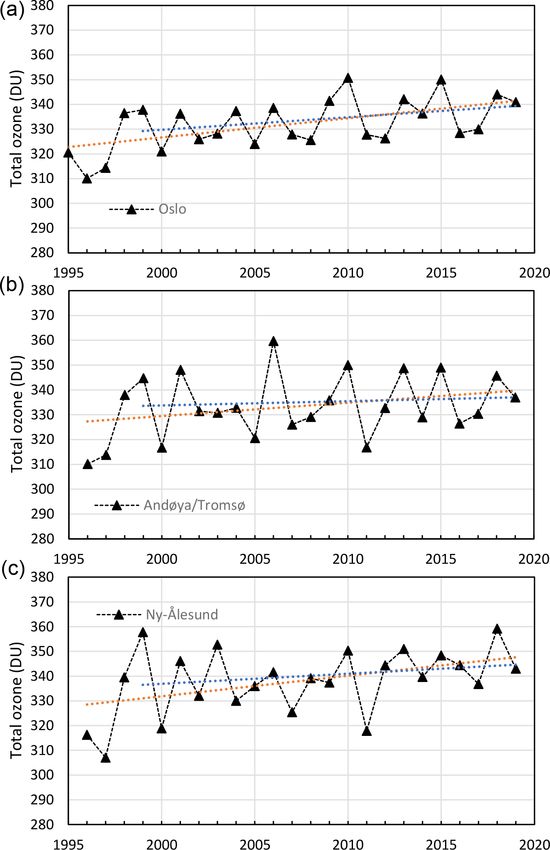
In Fig. 8, linear observational trends for the entire period
(from 1995/1996 to 2019) are marked in orange, whereas
changes for the last 20 years are marked in blue. The lat-
ter trend estimate is done to eliminate the years in the
mid-1990s with very low ozone, partly influenced by the
Mt. Pinatubo eruption and the cold Arctic winters in 1996
and 1997 (Solomon, 1999). The analysis reveals a total ozone
increase for the period 1995/1996–2019 at all stations and
for all seasons. However, only half of the positive trend re-
sults are statistically significant to a 95 % confidence level
(2σ ) – that is, annual trends in Oslo (2.3 ± 1.5 % per decade)
and Ny-Ålesund (2.5 ± 2.2 % per decade), the fall trend in
Oslo (3.4 ± 1.5 % per decade) and Andøya (3.0 ± 2.8 % per
decade), and spring values in Ny-Ålesund (3.8 ± 3.5 % per
decade). If we exclude the years 1995–1998 and only look at
Figure 8. Annual average total ozone in Oslo, at Andøya/Tromsø,
the changes for the period 1999–2019, the regression anal-
and in Ny-Ålesund. Linear trends for the whole period 1995/1996–
ysis still indicates an increase in total ozone during the last
2019 are marked with orange lines; ozone changes for 1999–2019
two decades. However, the increases are less pronounced and are in blue.
not significant at the 2σ level, except from the increase in
Oslo (3.2±2.0 % per decade) for fall. The annual TOC trends
for the 1999–2019 period are 1.5 ± 1.8 % per decade for
variability will reduce the statistical significance and can
Oslo, 0.5±2.6 % per decade for Andøya, and 1.2±2.4 % per
mask a potential trend in total ozone. The overall positive
decade for Ny-Ålesund. Results that are statistically signifi-
trend results from the three Norwegian stations agree well
cant are marked in bold in Table 6. Total ozone is strongly in-
with analyses from the Scientific Assessment of Ozone De-
fluenced by stratospheric circulation and meteorology, which
pletion: 2018 (WMO, 2018). Model simulations presented
give rise to large interannual variability in total ozone. This
in WMO (2018) conclude that about half of the observed up-
Atmos. Chem. Phys., 21, 7881–7899, 2021 https://doi.org/10.5194/acp-21-7881-2021T. M. Svendby et al.: GUV long-term measurements of total ozone column and effective cloud transmittance 7893 Figure 9. Total ozone column measured in Ny-Ålesund in spring 2020 with the SAOZ instrument (black triangles), GUV (black line), OMI satellite (orange line), and GOME-2 (blue line). per stratospheric ozone increase after 2000 is attributed to the good during this ozone loss period, indicating that GUV per- decline of ODSs since the late 1990s. The other half of the forms well even though the ozone profile used in the lookup ozone increase is attributed to the slowing of gas-phase ozone table did not match the actual profile that was observed above destruction cycles, which results from cooling of the upper Ny-Ålesund in March and April 2020. Figure 9 shows that stratosphere caused by increasing concentrations of green- the ground-based instruments, both GUV and SAOZ, in gen- house gases. It should be noted that stratospheric cooling re- eral give higher TOC than the satellites during February and duces Arctic ozone if the temperature drops below the thresh- parts of March 2020. There is also a notable difference be- old of formation of polar stratospheric clouds (PSCs), as ex- tween GOME-2 and OMI between mid-April and the end of emplified below. Normally PSCs will only exist between De- May. The satellite error estimates are around 4 % for these cember and March and therefore mainly affect ozone trends months, and as explained in Sect. 2 the ground-based instru- for winter and early spring. ments also have a significant uncertainty at SZA > 80◦ . This Despite a general increase in TOC during the last decades, demonstrates the challenges of performing accurate TOC Lawrence et al. (2020) reported that the TOC over the north- measurements in the Arctic. ern polar region was exceptionally low in late winter and Episodes of very low total ozone content are not limited early spring 2020. The average total ozone for February to to early spring and periods of several weeks. They can also April was the lowest value registered since the start of satel- occur for a few days because of unusual meteorological or lite measurements in 1979. The low TOC was partly caused atmospheric conditions, as observed at Kjeller in late 2019. by an exceptionally cold and persistent stratospheric polar In Fig. 10, GUV noontime total ozone from Oslo and Kjeller vortex, which provided ideal conditions for chemical ozone in 2019 is compared to GOME-2 and OMI data from Oslo destruction (Grooß and Müller, 2021; Manney et al., 2020; (12:00 UTC values). The black line shows GUV TOC data, Wohltmann et al., 2020). These low ozone values resulted whereas blue and orange lines represent GOME-2 and OMI in enhanced UV radiation, and the average UV index mea- measurements, respectively. The lack of GUV data from sured by the GUV instrument in Ny-Ålesund in April 2020 mid-May and June is caused by the calibration campaign was elevated by 34 % relative to the average 1979–2019 level at DSA (see Sect. 2.2). GUV data prior to mid-May 2019 (Bernhard et al., 2020). are from Oslo, whereas measurements after July 2019 were Figure 9 shows GUV total ozone in Ny-Ålesund from mid- performed at Kjeller outside Oslo. The GUV comparison to February to May 2020, and the low ozone levels from the end GOME-2 and OMI overpass data from Oslo indicates that the of March to mid-April are clearly seen. Total ozone values agreement between ground-based measurements and satel- from SAOZ, GOME-2, and OMI (TM3DAM v4.1) are in- lite data is as good at Kjeller as in Oslo. A very interesting cluded in the figure for comparison. The study from Wohlt- episode is the extremely low total ozone values measured mann et al. (2020) showed that the Arctic ozone at 18 km on 4 December 2019 (red circle in Fig. 10). On this day, altitude was depleted by up to ∼ 93 % in spring 2020, which the noontime GUV ozone value at Kjeller was only 193 DU. is comparable to typical local values in the Antarctic ozone This is the lowest value measured by the GUV instrument hole. The agreement between GUV, GOME-2, and OMI is in Oslo/Kjeller the last 20 years. GOME-2 and OMI from https://doi.org/10.5194/acp-21-7881-2021 Atmos. Chem. Phys., 21, 7881–7899, 2021
7894       T. M. Svendby et al.: GUV long-term measurements of total ozone column and effective cloud transmittance

Figure 10. Total ozone column values from Oslo/Kjeller in 2019 measured with the GUV instrument (black line), OMI satellite (orange
line), and GOME-2 (blue line). The red circle indicates the mini ozone hole over Scandinavia on 4 December 2019.

Oslo also measured very low total ozone at 12:00 UTC on
this day, 201 and 203 DU, respectively. At 18:00 UTC the
previous day the total ozone value from OMI was as low as
193.5 DU.
   In the fall/winter of 2019 the Arctic polar vortex formed
earlier than usual (Manney et al., 2020; Lawrence et al.,
2020). Temperatures were low enough for PSC formation
by mid-November 2019, earlier than in any previous year
since at least 2004. PSCs were visible over Norway dur-
ing a large part of winter 2019/20. However, in early De-
cember, chorine activation and associated chemical ozone
loss were still limited. Dameris et al. (2021) indicate that a
mini ozone hole over southern Norway on 4 December 2019             Figure 11. Total ozone column on 4 December 2019 at
was caused by advection of lower-latitude air masses and in-        12:00 UTC from the GOME-2A satellite (data downloaded from
creased tropopause height. Figure 11 shows total ozone from         http://www.temis.nl/protocols/o3field/o3field_msr2.php, last access
the GOME-2 satellite at 12:00 UTC on this day. As seen in           19 May 2021).
the figure, the TOC was below 200 DU in the middle parts of
Norway, northern Sweden, and southwestern Finland.

4.3    Trends in eCLT                                               change in eCLT is even more pronounced if we only con-
                                                                    sider the months from late spring and early summer (April–
As described in Sect. 2, the effective cloud transmit-              June), as shown in Fig. 13. For these 3 months the overall
tance (eCLT) expresses the effect of clouds, aerosols, and          decreases in eCLT are ∼ 15 % for April and May and 9 % for
surface albedo on the UV radiation reaching the ground. In          June. The decadal trend is −7.6 %, −7.2 %, and −3.6 % for
the present study an eCLT of 100 % represents a clear sky           April–June, respectively (Table 7).
with no surface reflection. An eCLT value above 100 % can              To examine possible monthly differences and changes in
occur in case of scattered clouds and/or enhanced surface re-       the cloud cover in Ny-Ålesund for the period 1995–2019,
flection, e.g. snow.                                                cloud data from the Norwegian Centre for Climate Services
   Figure 12 shows annual average noontime eCLT val-                (NCCS) have been utilized (see Sect. 2.1). NCCS cloud data
ues and trends at the three stations: Oslo (orange line),           at 12:00 UTC have been selected to reflect the period where
Andøya/Tromsø (grey/black line), and Ny-Ålesund (blue               GUV eCLT noontime values are measured. Figure 14 shows
line). Linear regression analyses indicate that there are no        the number of clear days for April (blue), May (orange), and
changes in eCLT at Oslo or Andøya. However at Ny-                   June (black) for the years 1995–2019. The average number
Ålesund, eCLT has decreased over the last 25 years, and             is ∼ 10 d for April, ∼ 7 d for May, and only ∼ 4 d for June.
a negative trend of 5 %–6 % is evident from Fig. 12. The            Naturally, there are some variations from one year to another,

Atmos. Chem. Phys., 21, 7881–7899, 2021                                               https://doi.org/10.5194/acp-21-7881-2021
You can also read