Assimilation of GNSS tomography products into the Weather Research and Forecasting model using radio occultation data assimilation operator ...
←
→
Page content transcription
If your browser does not render page correctly, please read the page content below
Atmos. Meas. Tech., 12, 4829–4848, 2019
https://doi.org/10.5194/amt-12-4829-2019
© Author(s) 2019. This work is distributed under
the Creative Commons Attribution 4.0 License.

Assimilation of GNSS tomography products into the Weather
Research and Forecasting model using radio occultation data
assimilation operator
Natalia Hanna1 , Estera Trzcina2 , Gregor Möller1,a , Witold Rohm2 , and Robert Weber1
1 Department   of Geodesy and Geoinformation, TU Wien, Vienna, 1040, Austria
2 Instituteof Geodesy and Geoinformatics, Wrocław University of Environmental and Life Sciences, Wrocław, 50-357, Poland
a now at: Ionospheric and Atmospheric Remote Sensing Group, Jet Propulsion Laboratory, California Institute of Technology,

Pasadena, CA 91109, USA

Correspondence: Natalia Hanna (natalia.hanna@geo.tuwien.ac.at)

Received: 30 November 2018 – Discussion started: 12 February 2019
Revised: 16 August 2019 – Accepted: 21 August 2019 – Published: 10 September 2019

Abstract. From Global Navigation Satellite Systems                  model, using its three-dimensional variational data assimi-
(GNSS) signals, accurate and high-frequency atmospheric             lation (WRFDA 3D-Var) system, in particular, its radio oc-
parameters can be determined in all-weather conditions.             cultation observation operator (GPSREF). As only total re-
GNSS tomography is a technique that takes advantage of              fractivity is assimilated in GPSREF, it was calculated as the
these parameters, especially of slant troposphere observa-          sum of the hydrostatic part derived from the ALADIN-CZ
tions between GNSS receivers and satellites, traces these           model and the wet part from the GNSS tomography. We
signals through a 3-D grid of voxels, and estimates by an           compared the results of the GNSS tomography data assim-
inversion process the refractivity of the water vapour con-         ilation to the radiosonde (RS) observations. The validation
tent within each voxel. In the last years, the GNSS tomog-          shows the improvement in the weather forecasting of relative
raphy development focused on numerical methods to stabi-            humidity (bias, standard deviation) and temperature (stan-
lize the solution, which has been achieved to a great extent.       dard deviation) during heavy-precipitation events. Future im-
Currently, we are facing new challenges and possibilities in        provements to the assimilation method are also discussed.
the application of GNSS tomography in numerical weather
forecasting, the main research objective of this paper. In the
first instance, refractivity fields were estimated using two dif-
ferent GNSS tomography models (TUW, WUELS), which                   1   Introduction
cover the area of central Europe during the period of 29 May–
14 June 2013, when heavy-precipitation events were ob-              Global Navigation Satellite Systems (GNSS) measurements
served. For both models, slant wet delays (SWDs) were cal-          of the microwave signals transmitted between the satel-
culated based on estimates of zenith total delay (ZTD) and          lites and the ground-based receivers are affected by the at-
horizontal gradients, provided for 88 GNSS sites by Geode-          mosphere (Hofmann-Wellenhof et al., 2001). The signals
tic Observatory Pecny (GOP). In total, three sets of SWD            are bent, attenuated and delayed in two atmospheric lay-
observations were tested (set0 without compensation for hy-         ers, namely the ionosphere and the troposphere (Böhm and
drostatic anisotropic effects, set1 with compensation of this       Schuh, 2013). As the effects caused by both of them can be
effect, set2 cleaned by wet delays outside the inner voxel          distinguished, the latter is referred to as the tropospheric de-
model), in order to assess the impact of different factors on       lay and stands for the signal delay integrated over the whole
the tomographic solution. The GNSS tomography outputs               ray path (Bevis et al., 1994; Kleijer, 2004; Mendes, 1999).
have been assimilated into the nested (12 and 36 km hori-           The tropospheric delay can be estimated from differenced
zontal resolution) Weather Research and Forecasting (WRF)           GNSS measurements. Therefore, it is usually modelled in

Published by Copernicus Publications on behalf of the European Geosciences Union.
4830                                                              N. Hanna et al.: Assimilation of GNSS tomography products

a vertical column above each station as zenith total delay           1997). Operational assimilation of STDs into the MM5 sys-
(ZTD) – i.e. the observed delay is mapped to the zenith di-          tem has shown a positive impact on the representation of wa-
rection and integrated over a certain period of time (Dach           ter vapour field and precipitation; a reduction of the spin-
et al., 2007). The tropospheric delay is related to the weather      up time of the model was also noticed (Bauer et al., 2011).
conditions in the vicinity of the GNSS station (pressure, tem-       An assimilation experiment carried out during a local heavy-
perature and humidity); therefore it carries valuable meteo-         rainfall event indicated that GPS–STD assimilation improved
rological information (Guerova et al., 2016).                        rainfall forecast significantly in terms of timing and inten-
   In the last years, a huge effort was made to utilize GNSS         sity, when compared to a GPS–ZTD and GPS–IWV assim-
measurements for operational weather forecasting; as a re-           ilation only (Kawabata et al., 2013). However, the issue re-
sult, several projects have been conducted to establish pro-         lated to the development of the observation operator for STD
cessing centres for a continuous estimation of the tropo-            has a high computational cost of its parts: forward opera-
spheric state using GNSS products (Elgered, 2001; Haase              tor, tangent linear and adjoint. The forward operator requires
et al., 2001; de Haan et al., 2009; Dousa, 2010; Karabatić          computing a ray-traced delay between the satellite and the
et al., 2011). In addition to ZTD, another tropospheric pa-          ground-based receiver for each STD observation. Another
rameter, namely integrated water vapour (IWV), has been              concern is the high nonlinearity of the signal path for low-
derived and assimilated into the numerical weather predic-           elevation satellites. In the result, the parameterization for the
tion (NWP) models (Falvey and Beavan, 2002; Gutman et                tangent linear operator is a complex problem and requires a
al., 2004). This parameter is calculated based on the wet part       number of iterations. Additionally, the adjoint operator re-
of ZTD (i.e. zenith wet delay, ZWD), and is strictly related to      quires interpolation of the increments to a number of nodes
the amount of water vapour in the troposphere; thus it is ben-       around the signal path. This procedure is computationally ex-
eficial for meteorological systems since a precise knowledge         pensive, as the signal traverses through the number of voxels
about humidity in the neural atmosphere is crucial for ac-           in an arbitrary direction (not only vertical). Moreover, simi-
curate weather forecasting (Andersson, 2018). Studies have           lar as with IWV and ZTD assimilation, the observation un-
shown that assimilation of GNSS products, either ZTDs or             certainty is difficult to assign. The STD observations are in-
IWVs, into operational NWP models usually has a positive or          tegrated over the GNSS signal’s path, with a different quality
neutral impact on the forecast of humidity, rain location and        of retrieval in particular parts of the model.
accumulated rain amount (Poli et al., 2007; Inness and Dor-             In contrast, if STDs are pre-processed using GNSS tomog-
ling, 2012; Bennitt and Jupp, 2012). Cucurull et al. (2004),         raphy principles, the outputs are profiles, similar to the obser-
Nakamura et al. (2004), Boniface et al. (2009), and Tilev-           vations for which the operators have already been developed
Tanriover and Kahraman (2014) demonstrated that the posi-            and operationally used in weather models, i.e., radio occulta-
tive impact is most significant during heavy-precipitation or        tion retrievals (Healy, 2007). It was demonstrated in a num-
storm events.                                                        ber of studies that these profiles increase the quality of model
   However, as the tropospheric parameters integrated into a         fields (Cucurull et al., 2007; Poli et al., 2010; Buontempo et
zenith direction reflect horizontal changes in meteorological        al., 2008; Healy, 2008). The quality of the refractivity pro-
parameters, they do not provide information about a verti-           files is relatively easy to obtain, e.g., by the comparison to
cal structure. In order to make better use of information that       the radiosonde profiles and assigning proper uncertainties to
is contained in the raw GNSS measurements, ZTD can be                the coinciding levels (Brenot et al., 2018).
mapped back into the direction of the satellites in view us-            Motivated by the increasing number of GNSS satellites
ing mapping functions. In addition, GNSS-derived horizon-            and the build-up of densified ground-based GNSS networks
tal gradients provide additional information about azimuthal         in the 1990s, Flores et al. (2000) proposed a processing
asymmetry, i.e. the horizontal structures in the troposphere         method, which allows for reconstruction of structural infor-
(Niell, 1996; Böhm and Schuh, 2004; Böhm et al., 2006).              mation from GNSS tropospheric parameters – also known as
While hydrostatic gradients are caused by differences in tro-        GNSS tropospheric tomography. This technique is one of the
pospheric height as well as regional variations in pressure,         most promising since it uses slant wet delay (SWD) obser-
wet gradients reflect local variations in the water vapour dis-      vations together with the principles of tomography to obtain
tribution. In contrast to wet gradients, hydrostatic gradients       not only the amount of water vapour, but also its distribution
are usually smaller and show fewer temporal variations (on           in space and time. For the inversion of the equation system
average < 0.1 mm every 3 h vs. 0.3 mm every 3 h for wet gra-         Flores et al. (2000) were using singular value decomposi-
dients; see Ghoddousi-Fard, 2009). In case horizontal gradi-         tion (SVD) methods together with constraints imposed on
ents are considered in the reconstruction of the GNSS signal         the system of equations (smoothing, boundary and vertical
delays for each GNSS satellite-receiver pair (along the in-          constraints). In the following years, a number of refinements
dividual signal path), slant total delays (STDs) are obtained,       in the technique have been implemented. Inclusion of sup-
which better represent the state of the troposphere, especially      plementary wet refractivity data from external data sources
in the case of strong horizontal humidity gradients during           into a functional model (Bender et al., 2011; Rohm et al.,
severe weather phenomena in frontal regions (Koch et al.,            2014; Benevides et al., 2015; Möller, 2017) resulted in sta-

Atmos. Meas. Tech., 12, 4829–4848, 2019                                                www.atmos-meas-tech.net/12/4829/2019/
N. Hanna et al.: Assimilation of GNSS tomography products                                                                    4831

bilization of the solution without need of smoothing con-           icated to the methodology of GNSS troposphere tomography
straints, which is especially important during severe weather       and provides a detailed description of the models used for to-
phenomena with high variability of water vapour in the tro-         mography processing. Section 4 introduces the methodology
posphere. A new approach of parametrization of the domain,          of tomographic data assimilation into the WRF model; fol-
using trilinear and spline functions instead of constant values     lowed by a description of the meteorological situation under
inside each volume element (voxel), showed the substantially        study in Sect. 5. In Sects. 6 and 7, the results of tomography
smaller maximum error of the solution (Perler et al., 2011;         and of the assimilation experiments are analysed. The main
Ding et al., 2018). Another approach, using the Kalman filter       conclusions are presented in Sect. 8.
instead of least squares (Rohm et al., 2014), led to better re-
sponsiveness to the severe weather. A number of experiments
have been carried out showing positive results for detecting        2   GNSS slant wet delays
heavy-precipitation events (Troller et al., 2006; Rohm and
                                                                    The Advanced Global Navigation Satellite Systems Tropo-
Bosy, 2009; Perler et al., 2011; Rohm et al., 2014; Adavi and
                                                                    spheric Products for monitoring Severe Weather Events and
Mashhadi-Hossainali, 2015; Chen et al., 2017). In addition
                                                                    Climate (GNSS4SWEC; http://gnss4swec.knmi.nl/, last ac-
to the development of technical aspects, which was widely
                                                                    cess: 15 October 2018) benchmark campaign has been or-
performed in the last years, GNSS tomography should also
                                                                    ganized within the EU COST Action ES1206 (Jones et al.,
be tested on its ability to fulfil the requirements of up-to-
                                                                    2018). This campaign provided both GNSS tropospheric
date weather prediction methods, i.e. on its suitability for as-
                                                                    estimates (with time resolution of 1 h for ZTDs and 6 h
similation into the NWP models (Innes and Dorling, 2012).
                                                                    for horizontal gradients) for 88 GNSS sites in central Eu-
The first research on this topic was carried out by Möller
                                                                    rope (see Fig. 2) and data used for validation (ALADIN-CZ
et al. (2015). Its aim was to transform wet refractivities de-
                                                                    data and radiosonde observations). The ZTDs and gradients,
rived by GNSS tomography into humidity and temperature
                                                                    which were utilized for the computation of slant wet delays
profiles and then assimilate them into the AROME NWP
                                                                    (SWDs), were estimated in a daily post-processing analysis.
model for a selected test period. Verification was made us-
                                                                    For more details about the GNSS processing strategy at GOP,
ing surface station measurements, radio sounding data, and
                                                                    the reader is referred to Douša et al. (2016, Sect. 5.1).
precipitation analysis. Tomography data assimilation results
                                                                       In a first step, the tropospheric parameters for 00:00,
compared with the results of ZTD data assimilation indi-
                                                                    06:00, 12:00 and 18:00 UTC have been selected. Afterwards,
cated a significantly larger impact of the new technique, es-
                                                                    for each epoch the zenith hydrostatic delay (ZHD) was com-
pecially within 6 to 12 h of the forecast (a drying effect in the
                                                                    puted by means of the Saastamoinen model (Saastamoinen,
AROME forecast field). As the results clearly showed the
                                                                    1972) and removed from the ZTD estimates:
potential of 3-D refractivity observations, another case study
has been performed by Trzcina and Rohm (2018), concern-             ZWD = ZTD − ZHD.                                           (1)
ing assimilation of a near-real-time (NRT) tomographic solu-
tion into the WRF model using an operator dedicated to radio        The required air pressure values have been derived from
occultation (RO) observations of total refractivity (GPSREF;        mesoscale ALADIN-CZ 6 h forecast data, as provided by the
Cucurull et al., 2007). Comparison with several external ob-        Czech Hydrometeorological Institute (CHMI), and spatially
servations has shown the positive impact within the 6 to 12 h       interpolated to each GNSS reference site.
of the forecast of humidity in autumn, but not in summer.              The zenith wet delays (ZWDs) and the horizontal gradi-
Such assimilation-oriented tomography data analyses are es-         ents (GN , GE ) were mapped into the direction of the GPS
sential for further research on the utilization of GNSS tropo-      and GLONASS satellites in view above 3◦ elevation angles.
sphere tomography output as a valuable data source for NWP          Even though Douša et al. (2016) have processed only GPS
forecasts.                                                          observations, we expect that projection in the direction of all
   In this work, we present the assimilation of a 3-D wet re-       satellites from both constellations will not increase the er-
fractivity field derived by the GNSS tomography technique           ror of SWDs significantly (Kačmařík et al., 2017). Therefore
into the WRF model using the GPSREF (Cucurull et al.,               and for the highest consistency with GNSS data processing,
2007) observation operator. The experiment was performed            the VMF1 mapping function (Böhm et al., 2006) was used
during a heavy-precipitation event in central Europe in or-         for mapping (mfw ) of the ZWDs, and the Chen and Her-
der to investigate the impact on the weather forecast. Two          ring (1997) gradient mapping function (maz ) was applied for
tomographic models (TUW, WUELS) and three different ap-             mapping of the horizontal gradient parameters as follows:
proaches of SWD data calculation were used, in order to as-
sess the impact of particular factors on the tomographic so-        SWD = ZWD · mfw (ε) + GN · maz (ε) · cos (α) + GE
lution. Then, the results of several tomographic approaches               · maz (ε) · sin (α) .                                (2)
were discussed in terms of assimilation impact. The structure
of the paper is as follows: Sect. 2 describes the derivation of     The elevation (ε) and azimuth angles (α) of each satellite
slant wet delays from GNSS measurements. Section 3 is ded-          in view have been computed from broadcast ephemerides.

www.atmos-meas-tech.net/12/4829/2019/                                                  Atmos. Meas. Tech., 12, 4829–4848, 2019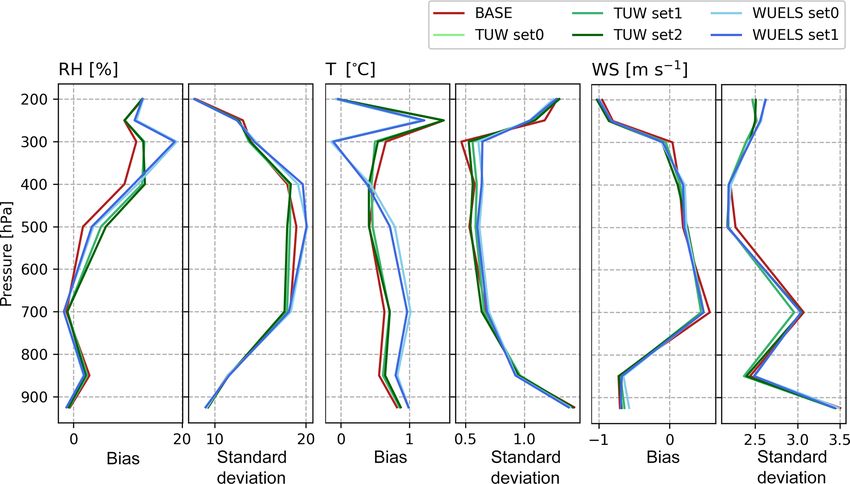
4832                                                               N. Hanna et al.: Assimilation of GNSS tomography products

                                                                      were determined, and the signal delay outside the inner voxel
                                                                      model was computed by ray-tracing through ALADIN-CZ
                                                                      6 h forecast data and finally removed from set0. As a con-
                                                                      sequence, the outer voxel model is not needed anymore for
                                                                      setting up the tomography model (see Sect. 3.1 for more de-
                                                                      tails).

                                                                      3   GNSS tomography
Figure 1. Hydrostatic component of azimuthal asymmetry, derived
from the ALADIN-CZ model data by ray-tracing.                         For conversion of precise integral measurements (like
                                                                      SWDs) into three-dimensional structures, a technique called
                                                                      tomography has been invented. According to Iyer and Hira-
                                                                      hara (1993) the general principle of tomography is described
No post-fit residuals were added in the reconstruction of the
                                                                      as follows:
SWD (Kačmařík et al., 2017). The resulting dataset of SWDs                Z
is hereafter referred to as “set0”.
                                                                      fs = g(s) · ds,                                           (3)
   Based on set0, two additional, more refined datasets
were derived, whereby “set1” compensates for hydrostatic                    S
anisotropic effects and “set2” was cleaned by wet delays              where fs is the projection function, g(s) is the object prop-
“outside” the inner voxel model (see Table 3 for further de-          erty function and ds is a small element of the ray path S
tails about the voxel model). In both cases, 2-D ray-tracing          along which the integration takes place. In order to adapt the
through ALADIN-CZ model level data (6 h forecast data)                tomography principle for GNSS tropospheric delay parame-
was carried for the determination of the hydrostatic delay            ters and to find a solution for Eq. (3), first the troposphere is
corrections. For more details about the applied ray-tracer, the       discretized in volume elements, named voxels, in which the
reader is referred to Möller (2017).                                  index of refraction is assumed to be constant and the ray path
   Within our study period (29 May–14 June 2013), we re-              is assumed to be a straight line. Further, by replacing fs with
trieved hydrostatic gradients < |0.7 mm|, which correspond            SWD and g(s) by wet refractivity (Nw ), the basic function of
to a signal delay up to |120 mm| at a 3◦ elevation angle. How-        GNSS tomography reads
ever, under specific conditions, hydrostatic gradients can be
as large as ±2 mm (see Zus et al., 2019), which corresponds                     m
                                                                                X
to a signal delay of about ∼ 34 cm (2 mm · 170) at a 3◦               SWD =           Nw,k · dk ,                                   (4)
                                                                                k=1
elevation angle. For set1, i.e. for compensation of hydro-
static asymmetric effects, ray-tracing was carried out through        whereby Nw,k is the constant wet refractivity and dk is the
ALADIN-CZ 6 h forecast data. Therefore, ray-traced delays             ray length in volume element k. In matrix notation Eq. (4)
were determined for each GNSS satellite in view, and for              reads:
equidistant azimuth angles (separated by 30◦ ; Landskron and
Böhm, 2018; Zus et al., 2019). From the obtained set of ray-          SW D = A · N w ,                                              (5)
traced hydrostatic delays, the mean hydrostatic delay was
computed and removed from the ray-traced hydrostatic de-              where SW D is the observation vector of size (n, 1), N w is
lay in the direction of the satellite in view. For more details,      the vector of unknowns of size (m, 1) and A is a matrix of
the reader is referred to Möller (2017), Chapter 6.3.                 size (n, m), which contains the partial derivatives of the slant
   Figure 1 shows the resulting hydrostatic asymmetric de-            wet delays with respect to the unknowns. Since Eq. (5) is
lays, as obtained for all observations within the study pe-           linear, the partial derivatives of SWD are the ray lengths (dk )
riod (29 May–14 June 2013). In a final step, the hydrostatic          in each voxel k. A solution for N w is obtained by inversion
asymmetric delays were removed from set0 to obtain set1.              of matrix A.
As the ALADIN-CZ model pressure error is 0.1 hPa with a
                                                                      N w = A−1 · SW D                                              (6)
standard deviation of about ±0.6 hPa (Möller, 2017), which
corresponds to a hydrostatic delay of about ±1.5 mm in the            Unfortunately in GNSS tomography, matrix A is usually not
zenith direction and up to 2 cm at a 3◦ elevation angle, the          of full rank (i.e. has zero singular values). As a consequence
obtained SWDs (set1) are widely free from hydrostatic ef-             Eq. (6) is ill-posed, i.e. not uniquely solvable. In order to find
fects.                                                                a solution for Eq. (6), truncated singular value decomposition
   Furthermore, for set2 the ray-tracer was applied for de-           (TSVD) methods are applied (Xu, 1998). Therefore, matrix
termining the slant wet delay outside the inner voxel model           A is split into three components:
(Fig. 2). Therefore, the intersection points between the GNSS
signal paths and the boundaries of the inner voxel model              A = U · S · VT ,                                              (7)

Atmos. Meas. Tech., 12, 4829–4848, 2019                                                    www.atmos-meas-tech.net/12/4829/2019/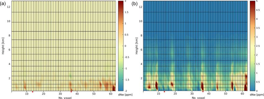
N. Hanna et al.: Assimilation of GNSS tomography products                                                                 4833

where U and V are orthogonal matrices and matrix S (n, m) is      Those residuals larger than 120 times the rms of the residu-
a diagonal matrix. The first m diagonal elements of S are the     als were discarded. The threshold was found empirically and
singular values (sk,k ); all other elements are zero. The ratio   allows for removal of large outliers (usually < 2 % of SWDs
between the largest and smallest singular values defines the      at a low elevation angle). The processing stopped after 10 it-
condition number κ(A) of matrix A.                                erations or before, if the change in rms was lower than 3 %
                                                                  or if the rms was lower than 0.5 mm.
          |smax |
κ (A) =                                                    (8)    3.2   Kalman filter solution (WUELS)
          |smin |

A condition number near 1 indicates a well-conditioned ma-        Estimation of the wet refractivity distribution in the WUELS
trix, a larger condition number indicates an ill-conditioned      solution was performed using TOMO2 software (Rohm and
problem. As a consequence, the tomography solution is sen-        Bosy, 2009, 2011; Rohm, 2012, 2013; Rohm et al., 2014;
sitive to observation errors, changes in the observation ge-      Zhang et al., 2015), based on a Kalman filter application. In
ometry, and also the solving strategy and its parameters de-      a first step, the state vector of wet refractivity N w and its
fined within the analysis. In the following, the two process-     covariance matrix P for epoch k were updated and based on
ing strategies as used for parameter estimation are described     the outputs form a previous epoch (k − 1):
in more detail. The general, underlying tomography settings
and input data are summarized in Table 3.                         N wk (−) = 8k N wk−1 (+) ,                               (10)
                                                                  Pk (−) = 8k Pk−1 (+) 8Tk   + Qk−1 ,                      (11)
3.1   Least-squares solution (TUW)
                                                                  where 8 denotes a state transition matrix, indicating pre-
The TUW tomography solution was calculated using the              dicted changes of the wet refractivity between consecutive
ATom software package (Möller, 2017). It is based on a least-     epochs; Q is a dynamic disturbance noise matrix. The state
squares adjustment, whereby each observation type is pro-         transition matrix is a diagonal matrix, set based on a priori
cessed individually as a partial solution (see Möller, 2017,      information for both epochs where
Eq. 7.46 ff.). This approach allows for proper truncated sin-
gular value decomposition (TSVD), whereby an eigenvalue                      N wapr k i,1
threshold of 0.006 km2 , found with the L-curve technique,        8k i,i =             .                                (12)
was set for singular value selection.                                       N wapr k−1
                                                                                       i,1
   Weighting of the GNSS slant observations was based
on the elevation angle (sin2 ε), with a standard deviation        The dynamic disturbance noise matrix was set based on mean
of 2.8 mm for the zenithal observations (ZTD). A height-          wet refractivity changes between epochs, calculated from
dependent weighting model was applied to the a priori wet         ALADIN-CZ model data for the whole period. The noise was
refractivity information, whereby the height-dependent stan-      calculated separately for each height level of the tomographic
dard deviations were computed by comparison of the a pri-         domain (see Table 3). After the prediction step, corrections
ori data with radiosonde data (stations 10 548, 10 771) and       to the state vector and its covariance matrix were computed
interpolated to the 15 height levels of the voxel model (see      from the observations. Hereby, the Kalman gain matrix K
Table 1). In the case where the altitude of RS station was        was defined as follows:
higher than the lowest tomographic layer (225 m), the values                                           −1
of temperature and specific humidity have been assumed to         Kk = Pk (−) ATk Ak Pk (−) ATk + Rk        ,               (13)
be constant.
                                                                  N wk (+) = N wk (−) + Kk (SW D k − Ak N wk (−)) ,        (14)
   The first two TUW solutions are based on SWD set0 and
set1. Therefore, the voxel model boundaries were defined ac-      Pk (+) = Pk (−) − Kk Ak Pk (−) ,                         (15)
cording to Table 3 and wet refractivity was estimated in both,
the inner and outer domain. In consequence, all available         where SW D stands for a vector of observations and R for
SWDs could be used for estimation of the wet refractivity         its covariance matrix. The vector of observations consists of
fields (set0 and set1). The third TUW solution is based on        two parts, the SWD observations and the a priori information
the SWDs of set2. For processing, the outer voxel model was       derived from ALADIN-CZ model data. Errors of the slant
removed since the outer tropospheric delay was already con-       delays mSWD are dependent on the elevation angle ε and were
sidered in preparation of set2. In consequence, all available     calculated using the following mapping function:
SWDs could be used and wet refractivity was estimated for                  mZWD
the inner voxel model (set2). Quality control was based on        mSWD =          ,                                        (16)
                                                                           sin(ε)
analysis of the SWD residuals (r).
                                                                  whereby mZWD = 10 mm is the assumed ZWD error (Kač-
ri = SWDi − Ai · Nw                                        (9)    mařík et al., 2017). Errors of the a priori information were

www.atmos-meas-tech.net/12/4829/2019/                                              Atmos. Meas. Tech., 12, 4829–4848, 2019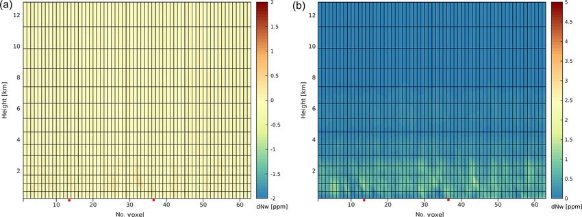
4834                                                               N. Hanna et al.: Assimilation of GNSS tomography products

computed by comparison with radiosonde observations (sta-             fine grid. In the two-way nest integration, the fine grid solu-
tions 10 548, 10 771, and 11 520), separately for each height         tion replaces the coarse grid solution for coarse grid points
of tomographic domain (Table 1). In the case where the al-            that lie inside the fine grid. The latest allows information ex-
titude of the RS station was higher than the lowest tomo-             change between the grids in both directions (Skamarock et
graphic layer (225 m), the values of temperature and specific         al., 2008).
humidity have been extrapolated.                                         In this research, the WRF model includes two domains
   For tomography processing, all available SWD observa-              (see Fig. 2): a parent domain (d01), which spans the area
tions above a 3◦ elevation angle were taken into account              of almost all of Europe, with 36 km horizontal spacing, and
and the signal paths were assumed to be straight lines. The           a nested domain (d02) within the area of central Europe,
WUELS tomography solutions (set0 and set1) are based on               with 12 km horizontal spacing (Fig. 2). The information be-
the SWD observations from set0 and set1, respectively. The            tween the domains flows in both directions (two-way nested
voxel model boundaries were defined according to Table 3              run). The vertical resolution of the model includes 35 pres-
(both inner and outer voxel model taken into account). A              sure levels, whereby the model top is defined at 50 hPa air
main quality indicator in the WUELS model was based on                pressure. The model background (initial and boundary condi-
a comparison of the SWD residuals (see Eq. 9). Observa-               tions) is provided by the National Centers for Environmental
tions with residual values ri larger than 3 times the standard        Prediction (NCEP) FNL (Final) operational global analysis
deviation were removed from the solution (approx. 4 % of              data with 1◦ × 1◦ horizontal resolution and 26 vertical lay-
observations, mainly at low elevation angles). The filter pro-        ers. These data are available at http://rda.ucar.edu/datasets/
cess was stopped after five iterations. Also, 14 stations with        ds083.2/ (last access: 10 March 2018).
a number of removed observations higher than 150 (for the
whole period) were rejected.                                          4.2   Assimilation operator

                                                                      Data assimilation is the technique by which observations are
                                                                      combined with an NWP product (the first guess or back-
4     WRF assimilation operator and settings
                                                                      ground forecast) and their respective error statistics to pro-
                                                                      vide an improved estimate (the analysis) of the atmospheric
4.1    WRF model
                                                                      (or oceanic, Jovian, etc.) state. Variational (Var) data assim-
The Weather Research and Forecasting (WRF) model is a                 ilation achieves this through the iterative minimization of a
mesoscale NWP system designed for both atmospheric re-                prescribed cost (or penalty) function. The aim of a variational
search and operational forecasting needs. It provides (1) two         data assimilation scheme is to find the best least-squares fit
different numerical cores (the Non-hydrostatic Mesoscale              between an analysis field x and observations y with an itera-
Model core (NMM) for operational use and the Advanced                 tive minimization of a cost function J (x):
Research WRF core (ARW) for research studies), (2) a data                    1                            1
                                                                      J (x) = (x − x b )T B−1 (x − x b ) + (y − H (x))T R−1
assimilation system, and (3) a software architecture enabling                2                            2
parallel computation and system extensibility (Schwitalla et                 (y − H (x)).                                        (17)
al., 2011).
   In the WRF model, a nest simulation can be performed.              In Eq. (17), x is a vector of analysis, x b is the forecast or
The nest is a finer-resolution model run, which can be em-            background vector (first guess), y is an observation vector,
bedded simultaneously within a coarser-resolution (parent)            B is the background error covariance matrix, H is an obser-
model run or run independently as a separate model fore-              vation operator, and R is the observation covariance matrix.
cast. The nested solution allows for the low-resolution model         The observation operator H , which can be non-linear, con-
to be run within the parent domain and the high-resolution            verts model variables to observation space. Differences be-
model to be run in the nested domain, which helps enhance             tween the analysis and observations/first guess are penalized
the efficiency of the model and reduces the time of calcu-            (damped) according to their perceived error.
lation of the high-resolution part of the model. Nesting also            In order to assimilate observations into the WRF data as-
enables us to run the model in a high-resolution very small           similation system, a special function, i.e. data assimilation
domain, avoiding a mismatch time and spatial lateral bound-           operator (H ), should be used. Although the WRF DA system
ary conditions (Skamarock et al., 2008). The coarse grid and          does not provide a direct assimilation operator for the GNSS
the fine grid can interact, depending on the chosen feedback          tomography wet refractivity fields, it is possible to apply a
option. Nested grid simulations can be produced using either          radio occultation operator (GPSREF) for the GNSS tomog-
one-way nesting or two-way nesting. In both, the one-way              raphy output data. The GPSREF assimilation operator is used
and two-way simulation modes, the fine grid boundary con-             to map model variables to refractivity space (Cucurull et al.,
ditions (i.e., the lateral boundaries) are interpolated from the      2007):

coarse grid forecast. In a one-way nest, the only information                                  P                   Pv
exchange between the grids comes from the coarse grid to the          N = Nh + Nw = 77.6           + 3.73 × 10⁵         ,      (18)
                                                                                               T                   T2

Atmos. Meas. Tech., 12, 4829–4848, 2019                                                 www.atmos-meas-tech.net/12/4829/2019/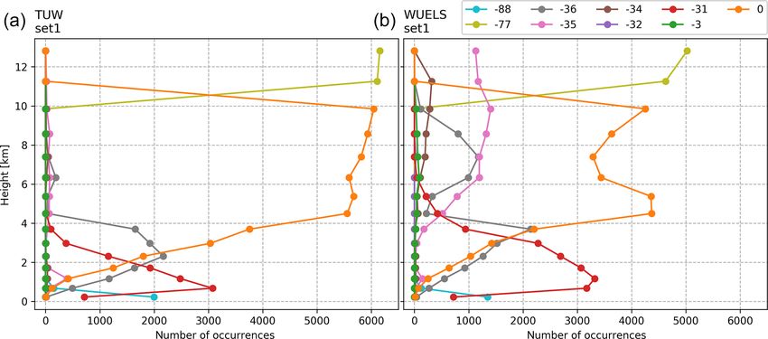
N. Hanna et al.: Assimilation of GNSS tomography products 4835
Table 1. A priori model error (m) and dynamic disturbance noise values (Q) as obtained by comparison of the a priori model data with
radiosonde data for each level of the TUW and WUELS tomography model.
Height (m) 225 675 1170 1715 2313 2972 3697 4494 5371 6336 7397 8564 9848 11 260 12 814
TUW m (ppm) 4.95 4.54 5.04 5.25 4.15 5.08 3.55 2.89 2.33 1.03 0.59 0.29 0.10 0.02 0.01
m (ppm) 10.57 5.56 5.40 5.95 5.48 4.55 4.29 3.25 2.41 1.65 1.12 0.57 0.23 0.06 0.02
WUELS
Q(ppm) 8.62 5.49 5.54 5.17 4.62 4.39 3.68 2.65 1.97 1.32 0.71 0.27 0.07 0.02 0.01
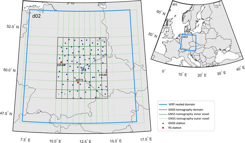
Figure 2. The geographical extensions of the WRF domains used in this research (d01 is coarse grid with 36 km horizontal spacing; d02 is
fine grid with 12 km horizontal spacing), GNSS tomography domain (grey line), together with inner (dark green line) and outer (light green
line) voxels, including GNSS sites (dark blue dots) and radiosonde stations (red squares).
where P is the total atmospheric pressure (hPa), T is the at- interpolated to each observation height. Finally, total refrac-
mospheric temperature (K), and Pv is the partial pressure of tivity field, i.e. the sum of Nh and Nw , is assimilated.
water vapour (hPa). The GPSREF operator enables assim-
ilation of total refractivity (N) at each observation height. 4.3 Assimilation settings
Since GNSS tomography provides Nw only, the hydrostatic
(dry) component of refractivity (Nh ) has to be modelled. The 3D-Var assimilation of five sets of tomography data
Therefore we use meteorological parameters (total atmo- (TUW set0, TUW set 1, TUW set2, WUELS set0, WUELS,
spheric pressure and atmospheric temperature) provided by set1) and the control run of the base weather forecast (with-
the ALADIN-CZ model. out assimilation) have been performed. In order to allow the
The ALADIN-CZ model is a local area, hydrostatic model NWP model to approach its own climatology after being
provided by Czech Hydrometeorological Institute (CHMI). started from the initial conditions (NCEP final data), the as-
Model simulations run at 4.7 km × 4.7 km horizontal resolu- similation was performed 6 h after model run (spin-up time).
tion and 87 hybrid-model levels. NWP model 3-D analysis The analysis has been performed at 00:00, 06:00, 12:00 and
fields are provided in GRIB format for 00:00, 06:00, 12:00 18:00 UTC. Each analysis includes an 18 h forecast with 1 h
and 18:00 UTC together with 6 h forecast fields with 1 h reso- resolution. Table 2 shows the data assimilation settings. In
lution (Kačmařík et al., 2017). In this study, the analysis data the process of assimilation, only the data from the voxels
of the ALADIN-CZ model are used to (1) compute pressure crossed by the GNSS signal were used.
values at the height of the GNSS station to reduce the hydro-
static part from the slant total delays (STDs) and (2) compute
temperature and pressure at the height of each Nwet observa- 5 Case study
tion in order to model the hydrostatic part of refractivity. In
order to calculate the hydrostatic component of refractivity, Our studies are based on the complex dataset collected within
the meteorological parameters provided by ALADIN-CZ are the European COST Action ES1206, as described in detail by
Douša et al. (2016). The study area comprises central parts of
www.atmos-meas-tech.net/12/4829/2019/ Atmos. Meas. Tech., 12, 4829–4848, 2019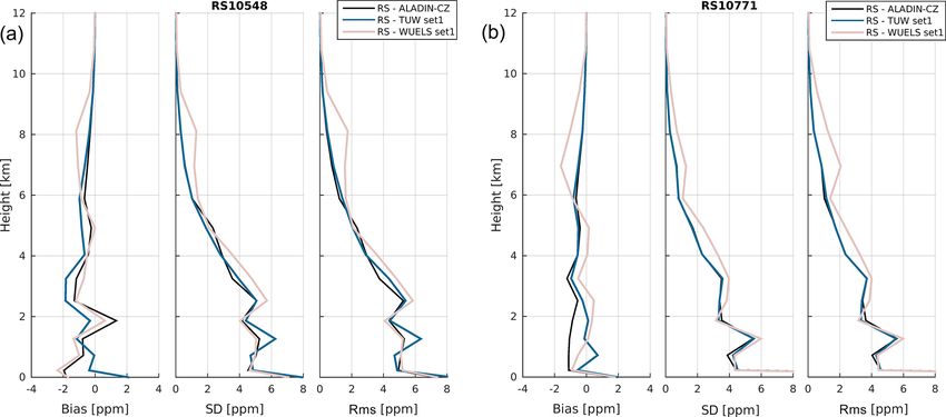
4836                                                               N. Hanna et al.: Assimilation of GNSS tomography products

Table 2. Applied data assimilation settings.

                   Horizontal resolution             parent domain: 36 km × 36 km
                                                     nested domain: 12 km × 12 km
                   Vertical layers                   35
                   Method                            3D-Var
                                                     radio occultation observation operator GPSREF
                   Initial and boundary conditions   NCEP FNL 1◦ × 1◦
                   Assimilation window               1h
                   Model run                         00:00, 06:00, 12:00, 18:00 UTC
                                                     6 h of model integration +18 h of forecast lead time
                   Physic options                    Yonsei University (YSU) scheme (Hong et al., 2006) for the atmo-
                                                     spheric boundary layer (ABL) parametrization;
                                                     Revised MM5 scheme (Jimenez et al., 2012) for surface layer;
                                                     unified Noah land surface model (Tewari et al., 2004);
                                                     Dudhia scheme for shortwave radiation (Dudhia, 1989);
                                                     Kain–Fritsch scheme for the cumulus parametrization (Kain, 2004)

Europe (Fig. 2). The study period (29 May to 14 June 2013)              identified within the inner model, with an average distance of
covers the events of heavy precipitation, which finally led to          48 km and altitude ranging from 70 to 885 m.
severe river flooding in all catchments on the northern Alpine
side (Switzerland, Austria, and southern Germany) and of the
mountain ranges in southern and eastern Germany as well as              6     Tomography results
in the Czech Republic.
   As reported by Grams et al. (2014), the core period of the           Based on the analyses carried out by Möller (2017), it is ex-
heavy precipitation occurred from 31 May 2013, 00:00 UTC                pected that the quality of the tomography wet refractivity so-
to 3 June 2013, 00:00 UTC. Within these 72 h, accumulated               lution differs significantly with model altitude. Thus, in the
precipitation of 50 mm was reported in regions of eastern               following the five TUW and WUELS tomography solutions
Switzerland, the Austrian Alps and the Czech Republic and               are validated against radiosonde measurements. In addition,
even exceeded 100 mm in several regions of the northern                 intra-technique comparisons highlight the impact of the to-
Alps. The events of heavy precipitation are connected to                mography settings on the obtained wet refractivity fields.
the presence of three cyclones: “Dominik”, “Frederik”, and
                                                                        6.1    Intra-technique comparison
“Günther”. These cyclones formed over (south)eastern Eu-
rope as a “cluster” with very similar tracks, and were rather
                                                                        Over the study period of 17 d, in total 68 tomography epochs
shallow systems with relatively high values of minimum
                                                                        (four solutions per day) have been processed for each tomog-
sea level pressure. These systems unusually track westward,
                                                                        raphy solution (TUW set0, set1, and set2 and WUELS set0
maintaining a northerly flow against the west–east-oriented
                                                                        and set1). Based on the wet refractivity differences between
mountain ranges in central Europe. However, within this pe-
                                                                        TUW set0 and set1, bias and standard deviation were com-
riod their movement was blocked by an anticyclone located
                                                                        puted for each voxel. Figure 3 shows the results for the 63
over the North Atlantic, which forced the cyclones to form
                                                                        (horizontal) × 15 (vertical) voxels of the inner voxel model,
an equatorward conveyor belt.
                                                                        whereby voxel number 1 indicates the lower southwest cor-
   The GNSS tomography solutions cover the region of east-
                                                                        ner and the voxel number 63 the northeast corner of the do-
ern Germany and western parts of the Czech Republic, in-
                                                                        main. The comparison between the TUW set0 and TUW set1
cluding the Erzgebirge (see Fig. 2). Within this area, the
                                                                        shows that the impact of anisotropy correction on the tomog-
equatorward-flowing warm air masses started to lift up,
                                                                        raphy wet refractivity field is very small (up to 1 ppm for bias
which goes along with a local maximum of precipitation of
                                                                        and standard deviation). For the WUELS model, the differ-
more than 75 mm within the core period of heavy precipita-
                                                                        ences reach maximally 2 ppm in terms of bias. In general, in
tion. For tomography processing, the study area was divided
                                                                        the case of standard deviation, the differences are up to 1 ppm
into an inner and an outer voxel model. The parameters of the
                                                                        (not shown).
tomography model and model settings are summarized in Ta-
                                                                           A similar analysis has been carried out for TUW set0 and
ble 3. From the benchmark dataset, 88 GNSS sites could be
                                                                        TUW set2 (Fig. 4). The major differences between both so-
                                                                        lutions are caused by the different approaches for compensa-

Atmos. Meas. Tech., 12, 4829–4848, 2019                                                    www.atmos-meas-tech.net/12/4829/2019/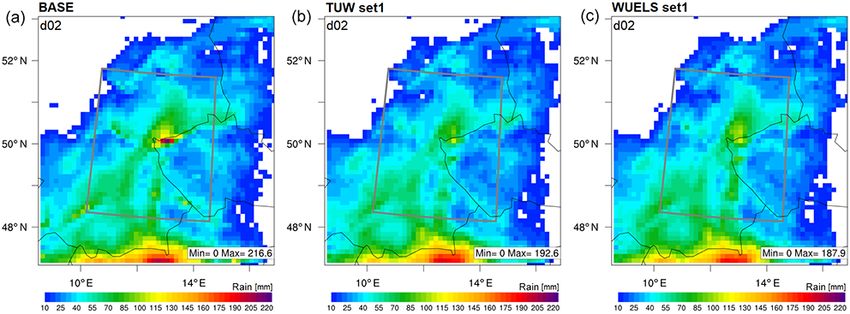
N. Hanna et al.: Assimilation of GNSS tomography products 4837
Table 3. Applied tomography model settings.
Period 29 May–14 June 2013
GNSS stations network number of GNSS sites: 88
average distance: 48 km
altitude of stations: 70–885 m
Tomography domain latitude: 48.5–52.0◦ (0.5◦ resolution, approx. 55 km)
longitude: 10.0–14.5◦ (0.5◦ resolution, approx. 43 km)
height: 225–12 814 m
outer voxel model: latitude ±1.5◦ (approx. 170 km), longitude ±3◦ (approx. 260 km)
A priori data ALADIN-CZ 6 h forecast:
horizontal resolution: 4.7 km × 4.7 km
vertical layers: 87 model levels
time of analysis: 00:00, 06:00, 12:00, 18:00 UTC
forecast ranges: 0, 1, 2, 3, 4, 5, 6 h
coordinates: non-rotated Lambert projection according to CHMI specification
SWD observations set0: SWDs (GPS + GLONASS, ZHD from ALADIN-CZ)
set1: SWDs (GPS + GLONASS, ZHD from ALADIN-CZ, hydrostatic gradients removed)
set2: SWDs (GPS + GLONASS, ZHD from ALADIN-CZ, outer delay removed)
Cut-off angle 3◦ elevation angle
Time settings every 6 h (00:00, 06:00, 12:00, 18:00 UTC)
Quality indicators TUW: outlier tests based on the post-fit residual rms
WUELS: filtration of dSWD based on synthetic data for detecting outlier observations
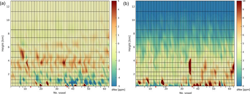
Figure 3. Bias (a) and standard deviation (b) of the differences in wet refractivity (ppm) between TUW set0 and TUW set1. Analysed period:
29 May–14 June 2013 (68 epochs). Red squares denote location of the RS stations.
tion of the outer voxel delay. While in set0 the tropospheric 18:00 UTC and 4 June, 18:00 UTC, larger standard devia-
delay in the outer voxel model was estimated, in set2 the tions were detected (up to 10 ppm; not shown). These varia-
outer delay was removed beforehand by ray-tracing through tions are caused by changes in the observation geometry but
ALADIN-CZ 6 h forecast data. Largest offsets between both also by changes in atmospheric conditions not described by
TUW solutions appear in northern parts of the study area the forecast data (error source in set2).
(voxel columns 55–63). In this part, the tropospheric delay Figure 5 presents the differences for bias and standard de-
is systematically overestimated (compared to ray-traced de- viation between both TUW set1 and WUELS set1. Since
lays) in the outer voxel model and consequently underesti- both tomography solutions are based on the same input data
mated in the inner voxel model. This leads to the positive bias (set1), similar wet refractivity fields are obtained. The largest
as visible in Fig. 4. In all other parts of the voxel model, the discrepancies are visible within the boundary layer, i.e. the
differences are widely averaged out over the study period of lowest 1–2 km of the atmosphere, and for the layer of 3–6 km
17 d. However, the standard deviation shows that variations height. The TUW solution tends to produce larger wet refrac-
over time cannot be avoided. Especially between 31 May, tivity fields in specific voxels near the surface (nos. 19, 20,
www.atmos-meas-tech.net/12/4829/2019/ Atmos. Meas. Tech., 12, 4829–4848, 2019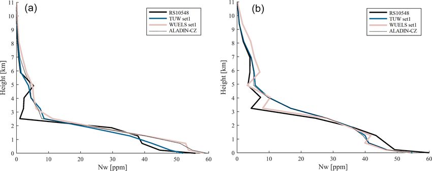
4838                                                               N. Hanna et al.: Assimilation of GNSS tomography products

Figure 4. Bias (a) and standard deviation (b) of the differences in wet refractivity (ppm) between TUW set0 and TUW set2. Analysed period:
29 May–14 June 2015 (68 epochs). Red squares denote location of the RS stations.

Figure 5. Bias (a) and standard deviation (b) of the differences in wet refractivity (ppm) between TUW set1 and WUELS set1. Analysed
period: 29 May–14 June 2013 (68 epochs). Grey triangles denote GNSS stations removed from the specific voxels of the WUELS solution
(one triangle stands for one rejected GNSS station), and red squares denote location of the RS stations.

24, 25, 35, 38, 41, 48, 50,. . .), in return slightly lower val-       deviation). The approach applied for the removal of the outer
ues in the two to three layers above, and then slightly higher         parts of the GNSS signal (i.e. set0 and set2) has a larger im-
values for the heights of 3–6 km (up to 5 ppm). Above the              pact on the results, however, not higher than 5 ppm in terms
6 km altitude, the absolute bias and the standard deviation            of the standard deviation. The presented analysis shows that
between TUW and WUELS solutions decrease significantly                 the greatest impact on the GNSS tomography results comes
(below 3 ppm). The discrepancies between both models are               from the applied model (TUW set1 and WUELS set1), where
caused by different approaches of the tomography settings.             the standard deviation is up to 10 ppm.
The tomography models differ in application of quality indi-
cators. In the WUELS approach, the GNSS stations that fre-             6.2   Time series of integrated zenith wet delays
quently failed quality check are removed from the solution,
whereas in the TUW solution all GNSS stations are taken                From the obtained wet refractivity fields, time series of
into account in every epoch. As a result, 14 GNSS stations             ZWDs were computed for the 88 GNSS sites within the study
were rejected from the WUELS model but not from the TUW                area by vertical integration using Eq. (19),
model. Locations of these stations within the voxel domain
are presented in Fig. 5 (grey triangles). In most cases, the                           Ht
                                                                                       X
locations of the rejected stations correspond with the largest         ZWD = 10−6           Nw · dh,                                 (19)
discrepancies between the models, e.g. voxel numbers 19,                               H0
37–40 and 45–49. Also, different weightings of the a priori
data were applied in both solutions, which results in notice-          where H0 is the height of the GNSS site and Ht is the height
able discrepancies between the outputs of the models.                  of the voxel top (at about 13.5 km height above mean sea
   Based on our analysis, we conclude that the removal of              level). Beforehand, Nw was horizontally linearly interpo-
the hydrostatic anisotropic effects does not significantly in-         lated from adjacent voxel centre points to the GNSS site and
fluence the tomographic outputs (approx. 1 ppm in standard             the vertical resolution was further increased to 20 m. Fig-
                                                                       ure 6 shows the derived ZWD time series for the entire study

Atmos. Meas. Tech., 12, 4829–4848, 2019                                                     www.atmos-meas-tech.net/12/4829/2019/
N. Hanna et al.: Assimilation of GNSS tomography products 4839
Figure 6. GNSS-derived (black) and tomography-derived (blue and
red) ZWD time series at GNSS site WTZR (Wettzell, Germany).
The dashed line shows the ZWD values derived from the ALADIN-
CZ model. The top plot shows the absolute values and the bottom Figure 7. Box plots of the ZWD differences for ALADIN-CZ,
plot highlights the ZWD differences with respect to the GNSS- TUW and WUELS models, compared to the GNSS data for all 88
derived ZWDs. sites.
control methods have a great impact on the results of tomog-
period of 17 d with 6 h temporal resolution, exemplary for raphy solutions.
GNSS site WTZR.
Both tomography solutions are more consistent with 6.3 Validation of tomography results with radiosonde
the GNSS-derived ZWDs than the ALADIN-CZ data. The data
ZWDs derived from ALADIN-CZ 6 h forecasts are occa-
sionally biased, a few hours “ahead” or “behind” the GNSS- Radiosonde measurements of temperature (T ) and dew point
derived ZWDs. The WUELS solution is negatively biased, temperature (Td ) were downloaded from https://ruc.noaa.
while discrepancies between GNSS and TUW are smaller gov/raobs/ (last access: 5 August 2018) for station 10 548
and the systematic error is reduced. Table 4 shows the statis- near Meiningen, Germany (lat: 50.57◦ , long: 10.37◦ , H =
tic of the ZWD differences for GNSS site WTZR but also the 450 m within voxel column no. 37), and 10 771 near Küm-
mean values over all 88 GNSS sites within the study domain. mersbruck, Germany (lat: 49.43◦ , long: 11.90◦ , H = 420 m
For both tomography models, the bias in ZWD is larger than within voxel column no. 13). The temporal resolution of the
for the a priori model (0.6 mm for TUW and −1.8 mm for measurements is 12 h (10 548) and 6 h (10 771), respectively.
WUELS), but the standard deviation is reduced (by 6.3 mm Dew point temperature and temperature were converted into
for TUW and by 4.1 mm for WUELS). water vapour e (Sonntag, 1990),
With respect to ZWD, both tomography solutions are 17.62·Td
closer to the GNSS solution than the a priori ALADIN-CZ e = 6.112 · e 243.12+Td , (20)
6 h forecast. In particular the standard deviation of the ZWD
differences can be reduced if GNSS tomography is applied and wet refractivity
(Fig. 7). e e
Figure 7 presents the box plots of the ZWD differences for Nw = k20 · + k3 · 2 , (21)
T T
all observations. The number of outliers for the ALADIN-
CZ model (141) is lower than for the tomography solutions with k20 = 22.9744 K hPa−1 and k3 = 375463 K2 hPa−1 (see
(275 for TUW and 314 for WUELS). This is a result of Rüeger 2002) best average. For comparison, the obtained
the higher value of standard deviation for the ALADIN-CZ profiles of wet refractivity (Nw ) were linearly interpolated
model than for the tomographic models. In addition, signif- to the voxel centre heights (see Table 1).
icant differences are visible between both tomography solu- Figure 8 shows wet refractivity profiles as obtained at ra-
tions. The WUELS solution tends to overestimate the water diosonde site RS10548 on 6 June 2013, 00:00 UTC and ra-
vapour content in the atmosphere slightly, which goes along diosonde site RS10771 on 13 June 2013, 00:00 UTC. Both
with a higher variability of the ZWD differences (about 2 plots were selected to highlight typical characteristics of the
times larger standard deviation than for the TUW solution). tomography solution. Due to proper weighting, the tomogra-
This shows that weighting of a priori data and applied quality phy solution can correct deficits in the a priori model (see
www.atmos-meas-tech.net/12/4829/2019/ Atmos. Meas. Tech., 12, 4829–4848, 20194840 N. Hanna et al.: Assimilation of GNSS tomography products
Table 4. Statistics of the differences in ZWD for GNSS site WTZR and all 88 GNSS sites within the study domain. The reference solution
(GNSS) was obtained by parameter estimation using GNSS phase measurements. The ALADIN-CZ, TUW set1 and WUELS set1 were
computed by vertical integration through the wet refractivity fields: Analysed period: 29 May until 14 June 2013.
GNSS minus ALADIN-CZ GNSS minus TUW GNSS minus WUELS
Bias(dZWD) SD(dZWD) Bias(dZWD) SD(dZWD) Bias(dZWD) SD(dZWD)
WTZR −0.5 mm 7.2 mm −0.9 mm 2.6 mm −2.5 mm 3.9 mm
ALL (88) 0.1 mm 9.1 mm 0.6 mm 2.8 mm −1.8 mm 5.0 mm
the lower 2 km of TUW set1 in Fig. 8a and the WUELS 7 Assimilation results
set1between 2 and 5 km height in Fig. 8b). Sharp changes in
wet refractivity can be recovered from TUW tomography so- 7.1 Diagnosis output
lution in the boundary layers and from the WUELS solution
in the mid-troposphere (related to weighting model). The to- The WRFDA system and the GPSREF operator are equipped
mography solutions are still affected by reconstruction errors with a quality control diagnostic tool, which allows for verifi-
(artefacts in the Nw profiles as visible in Fig. 8a between 2 cation of all input data before assimilation. As a result, not all
and 5 km height). of the refractivity observations are actually assimilated into
Figure 9 shows the corresponding statistics (bias, standard the model. Figure 11 presents a percentage of successfully
deviation and rms) over all analysed epochs (34 for RS10548 assimilated observations for each tomography set, as a func-
and 68 for RS10771) separately for each radiosonde site. tion of height. The height range with the largest number of
While RS10548 is located near a GNSS site, RS10771 lies assimilated observations is between 4 and 10 km. For these
within a voxel in which no GNSS site is located. Nonethe- heights, more than 90 % of observations of the TUW solu-
less, the quality of the tomography solution does not vary tions and about 50 %–80 % of those from the WUELS solu-
significantly according to the locations of RS stations. Up tion were assimilated. Below 4 km, the percentage of assim-
to 2 km height, the statistics for both tomographic models ilated observations grows systematically with height, from
are on the same level. In the upper parts of the troposphere, 0 % at the surface to 70 % for TUW and 40 % for WUELS.
the RS–TUW comparison shows similar accuracy as the RS– Above 10 km, no observations were assimilated, as they were
ALADIN-CZ data, whereas the standard deviation and rms removed in the quality control process.
of the WUELS model are noticeably higher. Since the comparison of tomographic observations with
Figure 10 shows the differences between TUW set0 and radiosonde data showed that in general the TUW solutions
TUW set2, separately for each radiosonde site. In fact, the have smaller errors than the WUELS solutions, the number
strategy for compensation of the outer delay has only a small of observations that passed the quality control is, in general,
impact on the tomography solution. Thereby, the impact is connected to the quality of the tomographic data. Because
independent from the location of the radiosonde site within of the restrictive quality control process in the GPSREF op-
the inner voxel model but mostly related to the tomography erator, some exception from this rule can be noticed in the
settings. The largest differences are visible in the lower 2 km lower (0–4 km) and the upper (10–12 km) troposphere, where
of the atmosphere. However, the overall impression is that almost all observations have been eliminated from the as-
set0 (estimation of the tropospheric delay in the outer voxel similation. The radio occultation observations, to which the
model) provides slightly better results than set2 (compensa- GPSREF operator is dedicated, very rarely reach the lowest
tion of the outer delay by ray-tracing through ALADIN-CZ level of the troposphere, whereas they are very accurate in
6 h forecast data). This is most likely related to the quality of the upper level.
the weather model forecast data during the period of extreme Apart from the number of successfully assimilated obser-
precipitation. Nevertheless, since both solutions are rather vations, the reason for the rejection was also studied. In the
close to each other, especially with respect to standard devi- quality control diagnostics of the GPSREF operator, each ob-
ation, only small improvements are expected by ray-tracing servation is assigned to one group, based on the information
through more reliable weather forecast data. of acceptance or rejection (and its cause). Figure 12 presents
the results of the quality control check separately for each
group and for each tomography solution as a function of
height in colour lines. For both tomography solutions, a large
number of observations is assigned to a group 0 (orange line)
that successfully denotes assimilated data. The number of ob-
servations from this group corresponds well with the one al-
ready presented in Fig. 11. The quality flags with numbers
Atmos. Meas. Tech., 12, 4829–4848, 2019 www.atmos-meas-tech.net/12/4829/2019/N. Hanna et al.: Assimilation of GNSS tomography products 4841
Figure 8. Wet refractivity profiles derived from radiosonde launches, ALADIN-CZ 6 h forecast data, TUW and WUELS tomography set1
for 6 June 2013, 12:00 UTC (a) and 13 June 2013, 00:00 UTC (b).
Figure 9. Statistics of the differences in wet refractivity at radiosonde sites RS10548 (a) and RS10771 (b).
−88, −77 and −3 are the general flags of the WRFDA sys- −32 (above 7 km, purple line). Additionally, if an observa-
tem, whereas the numbers from −31 to −36 are the flags tion gets the flag −31, all observations in the same vertical
assigned by the GPSREF operator. profile (same latitude and longitude) below that observation
The general flags with numbers −88, −77 and −3 respec- are also assigned to the flag −31 and they are not assimi-
tively denote data below the model’s terrain, data laying out- lated into the model. For the TUW model, the largest num-
side the horizontal domain and data failing maximum error ber of observations with flag −31 is at a height of 0.675 km
check. Observations assigned to the first group (blue line) oc- (about 3000 observations); this number systematically de-
cur in the surface layer only, about 2000 observations for the creases with height, to about 0 observations at 4 km. For the
TUW model and 1200 for the WUELS. The second group WUELS model, the largest discrepancies between the ob-
(yellow line) includes observations from the two highest lay- servations and the background occur between the heights of
ers (11 260 and 12 814 km). The number of observations as- 0.675 and 2.972 km (2000–3000 observations); no significant
signed to the third group (green line) is about 0 at all heights; discrepancies are noticed above 6 km. The second type of
only for the WUELS model at heights of 4–8 km does the quality check inside the GPSREF operator is based on a re-
number slightly grow up to about 50 observations. fractivity lapse rate (Poli et al., 2009). The −34 flag (brown
The quality flags assigned by the GPSREF operator (from line) is assigned to the observations where dN dz is smaller
−31 to −36) are connected with the values of assimilated −1
than −50 km , whereas the −35 flag (pink line) indicates
refractivity data. The first type of diagnostics is based on 2
observations where an absolute value of ddzN2 is larger than
the comparison between the assimilated observations and the
100 km−2 . For the TUW model, there are no observations re-
background values of refractivity (Cucurull et al., 2007). The
jected from the assimilation based on the lapse rate of refrac-
discrepancies between the two refractivity values should not
tivity. This indicates internal coherency of the model’s out-
be larger than 5 % (below 7 km) or 4 % (7–25 km) of the
put. In the WUELS model, for each layer above 6 km, more
mean value. Observations that do not meet this requirement
than 1000 observations were rejected from the assimilation
are assigned to the group −31 (below 7 km, red line) or
www.atmos-meas-tech.net/12/4829/2019/ Atmos. Meas. Tech., 12, 4829–4848, 2019You can also read


