Similarity Analysis to aid decision making on NBA Draft

Similarity Analysis to aid decision
 making on NBA Draft

 Miguel Alejandro Houghton López

Bachelor’s Degree Final Project in Computer Science and Engineering

 Facultad de Informática
 Universidad Complutense de Madrid
 2019 - 2020

 Director: Dra. Yolanda García Ruiz

 1

Análisis de la similaridad para la toma
 de decisiones en el Draft de la NBA

 Miguel Alejandro Houghton López

 Trabajo de Fin de Grado en Grado de Ingeniería Informática

 Facultad de Informática
 Universidad Complutense de Madrid
 2019 - 2020

 Director: Dra. Yolanda García Ruiz

 2

Contents
List of figures 3
List of tables 4
Abstract 5
Keywords 5
Resumen 6
Palabras clave 6

1. Introduction 7
 1.1 Motivation 7
 1.2 Objectives 9
 1.3 Methodology and work organization 9

2. State of the art 11
 2.1. Related work 11
 2.2. Clustering techniques 15

3. Software tools 17
 3.1. R, Rstudio y libraries 17
 3.2. Microsoft Power BI 18
 3.3. Github 18
 3.4. Others 19

4. Data source, methods and techniques 20
 4.1. Data collecting and integration 21
 4.2. Cleaning and data preprocessing 25
 4.3. Clustering techniques: analysis and visualization 27

5. Results 36
 5.1. Clustering analytics results 36
 5.2. Clustering Visualization results 45

6. Conclusions and future work 51
7. References 52
 3

List of figures
Figure 1. NBA Draft
Figure 2. Tankathon
Figure 3. NBA official
Figure 4. Basketball Reference
Figure 5. 2013 Draft dataset
Figure 6. Draft Combine All Years dataset
Figure 7. Players Shooting dataset
Figure 8. Seasons Stats dataset
Figure 9, Lot of Players dataset
Figure 10. Flowchart Single Linkage
Figure 11. Example Single Linkage
Figure 12. Kmeans data computed
Figure 13. Selection K number for NBA 2009
Figure 14. Chernoff faces characterization matrix
Figure 15. Dendrogram FT% on 3 features
Figure 16. Dendrogram FT% on 6 features
Figure 17. NCAA Overall shooting
Figure 18. NBA Overall shooting
Figure 19. Scaling dataset
Figure 20. Clustering NBA 2009
Figure 21. Selection K number for the merged dataset
Figure 22. Clustering vector NBA for the merged dataset
Figure 23. Clustering chart NBA for the merged dataset
Figure 24. Clustering vector NCAA for the merged dataset
Figure 25. Clustering chart NCAA for the merged dataset
Figure 26. Chernoff faces NBA 2009 for Height, Wingspan, Standing reach
Figure 27. Chernoff faces NBA 2009 for bench, agility and sprint
Figure 28. Chernoff faces NBA 2009 for weight and body fat
Figure 29. Chernoff faces NBA 2009 for vertical tryouts
Figure 30. PowerBI: Different shooting stats among a great set of players
Figure 31. PowerBI: Results over Draft 2009
Figure 32. PowerBi: Filtered results over 2009 Draft

 4

List of tables

Tabla 1. Data sources

Tabla 2. Variables of interest

 5

Abstract

This work is based on the different statistical studies published by Mock Draft Websites
and on webs that store the official statistics of the NBA players. The data associated with
NBA players and teams are currently very precious since their correct exploitation can
materialize in great economic benefits. The objective of this work is to show how data
mining can be useful to help the scouts in this real problem. Scouts participating in the
Draft could use the information provided by the models to make a better decision that
complements their personal experience. This would save time and money since by simply
analyzing the results of the models, teams would not have to travel around the world to
find players who could be discarded for the choice. In this work, unsupervised grouping
techniques are studied to analyze the similarity between players. Databases with statistics
of both current and past players are used. Besides, three different clustering techniques
are implemented that allow the results to be compared, adding value to the information
and facilitating decision- making. The most relevant result is shown at the moment in
which the shooting in the NCAA is analyzed using grouping techniques.

Keywords: Draft NBA, Basketball, Clustering analysis, Chernoff faces, R programming.

 6

Resumen

Este trabajo se basa en los diferentes estudios estadísticos publicados en páginas web de
predicción de Drafts de la NBA y en webs que almacenan las estadísticas oficiales de los
jugadores de la NBA. Los datos asociados a los jugadores y equipos de la NBA son
actualmente muy valiosos ya que su correcta explotación puede materializarse en grandes
beneficios económicos. El objetivo de este trabajo es mostrar cómo la minería de datos
puede ser útil para ayudar a los entrenadores y directivos de los equipos en la elección de
nuevas incorporaciones. Los ojeadores de los equipos que participan en el Draft podrían
utilizar la información proporcionada por los modelos para tomar una mejor decisión que
la que tomarían valorando su experiencia personal. Esto ahorraría mucho tiempo y dinero
ya que, simplemente analizando los resultados de los modelos, los equipos no tendrían
que viajar por el mundo para encontrar jugadores que pudieran ser descartados para la
elección. En este trabajo se estudian técnicas de agrupación para analizar la similitud entre
jugadores. Se utilizan bases de datos con estadísticas de jugadores tanto actuals como del
pasado. Además, se implementan tres técnicas de clustering diferentes que permiten
comparar los resultados, agregando valor a la información y facilitando la toma de
decisiones. El resultado más relevante se muestra en el momento en el que se analiza el
tiro en liga universitaria mediante técnicas de agrupación.

Palabras clave: Draft NBA, Baloncesto, Análisis Clúster, Caras de Chernoff, Programación
en R.

 7

Chapter 1. Introduction

1.1 Motivation
Technology have brought us new ways of transmitting digital information. Social media,
websites, smartphones and smartwatches are some tools that allow us to manage huge
amounts of data. All these data are useful for any business and are a very valuable asset.
It’s a great way to improve and develop new ways of earning economic power and
innovate in any area of a company. Descriptive data analysis and predictive data analysis
have become two of the best ways of studying new patrons and behaviors in the
information and helped the different business to innovate. But the data exploitation is not
only done in the business world. In recent years, data has taken a center stage in the sports
sector and is currently a very important part of any sports activity. Athletes are great
generators of data, and without a doubt, the world of sports is undergoing a
transformation. In any sports event, such as a football or basketball game, around 8
million events and data are generated (field condition, goals, jumps, distances traveled,
sanctions, players' fitness, passes, dribbles, etc.). The treatment of this information offers
the opportunity to make the most appropriate decisions, such as choosing a strategy during
a match, improving performance, substitute a player to prevent injuries, transfer
management, etc. For this, it will be necessary to apply the most modern statistical and
computational methods.

 In recent years, sports analysis has become a very attractive field for researchers.
In [1] they collect psychometric data on athletes during their competition season to study
how anxiety and mood influence the performance of players. Image recognition is used
to monitor the position and movement of players in real time. This information allows
inferring other data like the player's speed, distances between players, etc., very valuable
information for coaches. Applying modern statistical and computational techniques to the
data obtained from previous matches, it is possible to detect patterns in the competitors.
Consequently, coaches can predict the decisions of the opposing team and modify their
own tendency. The use of sensors in athletes (see [2]) allows a large amount of data to
be collected during training (level of fatigue, heart rate, etc.). The processing of this data
can be used to design personalized training routines. The digital trail that athletes leave
 8

on social networks is also valuable information for Clubs when making signings, since
with the analysis of behavior it is possible to predict whether an athlete will give the Club
a good or bad image in the future. Signing a star player can be expensive and a great risk
if he is injured or has a bad image.

 Basketball is one of the biggest sports in the world. Nowadays, is the sport that
has the most impact in the economy worldwide. Thanks to great basketball leagues such
as NBA, Euroleague, ACB or CBA, basketball moves billions of dollars every year. For
example, one of the most valuable teams in the NBA, the New York Knicks, has an
average value of 4 billion dollars. One of the biggest issues about every general manager
is concerned, is the optimal composition of their teams. Building the best team possible
according to the budget of any team is a complex process to accomplish. To do this, the
team management must take into account several factors such as everything related to the
players (physical, age, statistics), as well as everything related to the economic power of
the team (renewal of contracts and salary limits for instance). In addition, in the NBA, to
give dynamism to the league and make it as even as possible, Draft night is held every
year. This event consists of the selection of the best university or other league players to
become part of an NBA team. Teams place a high value on Draft, given that on numerous
occasions their primary choice on Draft night can shape the future of an entire franchise.

 The night of the Draft consists of two rounds, of 30 players each. The first
elections in the first round are divided by lottery among the 16 teams not classified for
the NBA playoffs. The rest of the elections of the round go to the teams classified in the
playoffs of the previous season. The draw to know which position each team chooses in
the Draft is called the 'NBA Draft Lottery' and the chances of choosing higher positions
depend on the number of losses in the regular season of the previous year. Given the
importance of this choice, management teams invest a lot of time and money in getting
the best possible choice for the position that has been obtained in the Draft. This choice
is conditioned by the needs of each team at all times. For example, if a team has a solid
player in the Center or Power-Forward position, the wisest course would be to 'draft' a
smaller player to cover the shortcomings of the team.

 9

The objective of this work is the design and analysis of different statistical models based
on real statistics. The teams participating in the Draft could use the information provided
by the models to make a better choice and not only based on personal intuition. This would
save time and money, since by simply analyzing the results of the models, teams would
not have to travel around the world to find players who could be discarded for the choice.

1.2 Objectives
The general objective of this work is to show how data mining can be useful in a real-life
problem as it is the Draft problem. More specifically, this work aims to carry out a follow-
up and a complete study of each Draft class in order to help teams to choose the best
player, based on real statistics and visualizations of data mining analytics as a complement
to the expertise of the basketball scouts.

1.3 Methodology and work organization
During the development of this study, I’ve noticed the great influence of the knowledge
acquired on my studies of Computer Science, especially thanks to subjects like
‘Statistics’, ‘Data Mining and Big Data Paradigm’ and ‘Data Bases’. In general terms, the
critical vision that gives you the development of the different areas of the degree has been
essential for this essay. Thanks also to some subjects of the degree related to
programming, I’ve been able to install and develop all the code necessary to carry out this
project. The methodology used in this Final Degree Project is to carry out the following
tasks:

1. Search of information and state of the art.
2. Location and download of required datasets in the study.
3. Cleaning and integration of datasets.
4. Documentation of data.
5. Installation of the necessary software tools and libraries.
6. Study of the applications and contact with the data.
7. Analysis of the data using the available libraries and own code.
8. Visualization of results.
9. Writing this report.

 10

This work is structured in the following way. Chapter 2 presents the state of the
art providing a critical vision of the apps and other work available. Besides it includes a
general description of the clustering techniques that we choose for the study. Chapter 3
describes the materials, datasets and software tools that have been used throughout the
project. Chapter 4 explains the statistical methods and measurement techniques used from
a theoretical point of view. Chapter 5 shows the results obtained after applying these
techniques. Finally, the conclusions and future work are proposed in Chapter 6. The
bibliography necessary to complement the information is also included, which is also a
reference to the sources of information used in this work.

 11

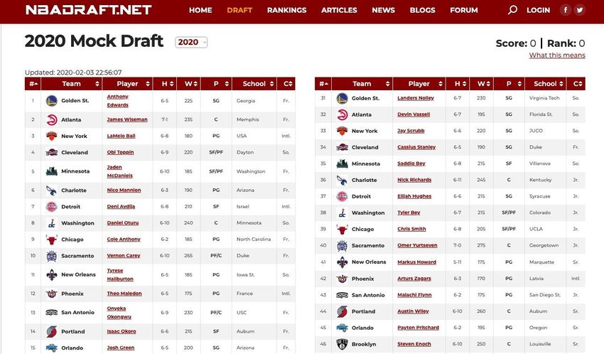
Chapter 2. State of the Art

This study is based on the different statistical studies made by Mock Draft Websites and
on webs that store the official statistics of the NBA players. The data associated with
NBA players and teams are currently very precious, since their correct exploitation can
materialize in great economic benefits. Along the lines of our work, there are several
companies that perform sophisticated analytics as a result of complex game and team
studies, and which are subsequently published on their websites for consumer
consumption. In general, these companies use a wide variety of data; data related to the
physical conditions of the players (height, weight, injury history, etc.) and data collected
during games. Many of these companies predict player selection in the NBA Draft.

 As we can suspect, this statistical information is of great value in the betting sector
since the fans guide their betting decisions in each Draft based on the information cooked
by these companies. These websites have a great influence on the betting industry because
every year the NBA Draft bets move millions of dollars. You can also look for Databases
that store lots of stats of active and inactive players. The fact that you can use the data
from retired players can make the study way more complete, because thanks to this, we
are going to be able to compare the prospects with any player who has ever played.

 This chapter is divided into two sections. The first is dedicated to existing
applications whose objective is related to that of the present work. Although the objective
of this work is not to implement an application of this type, its analysis is helpful to
understand all the elements of the study. The second section is dedicated to grouping
techniques. In addition to an introduction to these techniques, the techniques used at work
are explained in more detail and the results of which are presented in the corresponding
chapter.

2.1. Related work
In this section the most known Draft prediction and NBA stats websites are described.
Every item contains details of the most important features.

  NBADRAFT.NET
The company Sports Phenoms.Inc [3] publishes on its website (see Figure 1) a complete
analysis of players who will participate in the next NBA Draft. For each player, not only

 12

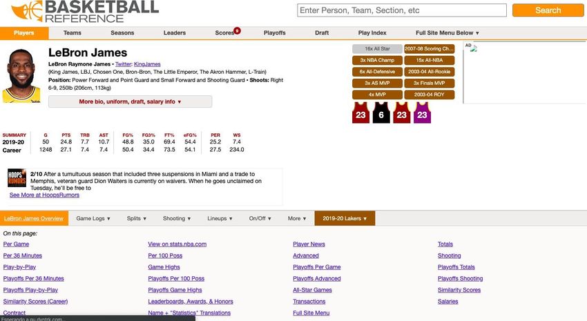
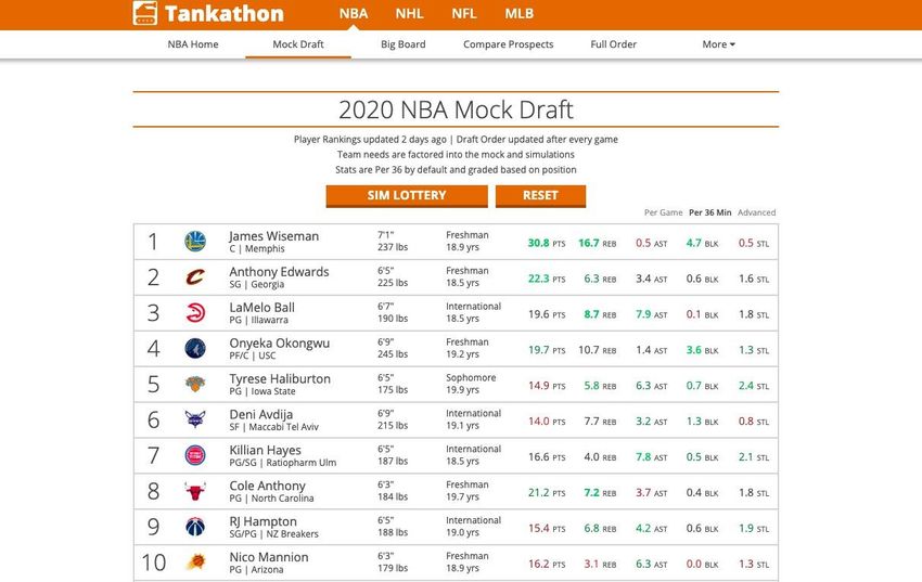
physical characteristics such as height and weight are included, but also different
characteristics related to game statistics, the team to which he belongs, information on
nationality and many others are presented. This website allows fans to create an account
and make their own drafts according to their own criteria and based on the information
contained on the page. Player rankings based on the different categories to which they
belong are also shown, such as High School players, NCCA players and International
players among others. The way in which this website extracts data is not too clear. Each
website has different prediction models and, although they are probably similar, they hide
their way of obtaining data from the public to prevent competition from benefiting.

Figure 1. Nbadraft.net 2020 web site

  TANKATHON.COM

The company Tankathon [4] offer a web site (see Figure 2) even more complete: one can
make predictions for any player but for the right amount of minutes played that you want.
It is updated every 2 days, and it's clear and simple interface makes an easy experience
for the user. It also makes predictions of the Draft Lottery, without taking into account
the players yet. In addition, it allows you to perform a large number of actions, such as
comparing players and consulting previous editions of Draft, with complete statistics both
per game and per approximations for 36 minutes of play.

 13

In addition, it is not limited only to the NBA, but rather goes further and offers these same
services for the rest of the major American leagues, such as the NHL (ice hockey), the
NFL (American football) and the MLB (baseball), where a player selection process is also
carried out using Draft.

Figure 2. Tankathon.net 2020 web site

The ways to obtain the models on this page are more accessible to the public, such that in
the 'Power Rankings' section where you can see the rankings generated by the Web model,
explain how it is to obtain the ranking including complete explanations and visuals to
which users have access. For example, Aaron Barzilai, who was a player on the varsity
basketball team at MIT before earning his Ph.D. in Mechanical Engineering at Stanford
University, wrote this article [5] where he concludes that:

 “The right to draft with a given pick in the NBA draft is an important but often
 overlooked topic in basketball analytics. .... The position of a team in a future
 draft is not known until the end of the season before that draft, and many trades
 involve picks multiple seasons into the future. Additionally, the strength of a future
 draft class is particularly hard to quantify. Finally, when valuing a pick a team

 14

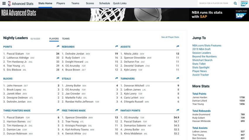
might include an estimation of their skill or their trading partner’s skill in drafting
 players.”

  STATS.NBA.COM:

This is the official stats website [6] of the NBA. It shows a great amount of different
advanced stats (see Figure 3), allowing you to compare how two different players are
playing together or how they are playing separated. This website will be used to compare
the ideal stats of the player that we would want for any team with any player of the actual
Draft Class that we are studying. This website uses a SAP data collection model created
specifically for sports statistics, which is not accessible to the public. Is called SAP Global
Sports One. SAP is at the forefront of transforming the sport and entertainment industries
by helping athletes, performers, teams, leagues, and organizations run at their best.

Figure 3. NBA official 2020 web site

  BASKETBALL-REFERENCE.COM

This web [7] stores every kind of stats for any player who has ever played in the NBA.
BasketBall-Reference (Figure 4) will be used in a similar way compared to stats.nba.com,
but adding the advantage of having advanced stats of retired players, which could make
the study more advanced and complete. The data sets on this page are open to the public
and offer the download of all the tables that make up the web page in different formats to
make it as accessible as possible to users. It is the best-known website for NBA statistics

 15

(it has variants dedicated to other sports and university sports). It offers complete statistics
on Playoffs, Draft, candidate approaches to MVP, ROY (rookie of the year), etc.

Figure 4. Basketball Reference 2020 web site

 In addition to the information collected on these applications and websites, studies
carried out at universities have also been analyzed, such as the aforementioned work by
[5] and more recently the work by Adhiraj Watave at the University of California,
Berkeley entitled Relative Value of Draft Position in the NBA [8].

2.2 Clustering techniques

Clustering algorithms consist of grouping the observations in sets trying to maximize the
similarity between the elements of the groups. For this, the distance between the different
variables of the observations is measured. Consequently, members of the same group have
common characteristics. These common characteristics also serve to characterize the
group. To obtain good results, it is necessary that the number of variables associated with
the observations are sufficiently descriptive. On the one hand, the results of the grouping
depend on the number and quality of the variables. The existence of dependent variables
or with little variability, adds noise to the system. On the other hand, the object of
grouping must also be taken into account when choosing variables. An objective may be
to detect inherent groups, but we may also be interested in finding representatives of
homogeneous groups or in detecting outliers. Hierarchical grouping methods based on

 16

distances have been used in this work. These methods do not require prior information
about the groups, called clusters, and are therefore called unsupervised methods. In this
work we use the Chernoff faces [9-13], Singlelinkage [14] (with dendograms) and
Kmeans methods [15, 16]. The idea of using these methods has been motivated by
Professor Krijnen's work on similarity in gene observations [17]. Krijnen uses the
database of Golub99 [18] to show how to find similarities by making groupings between
observations from people with different types of leukemia.
 The results of hierarchical grouping techniques are visualized using dendrograms.
These objects are trees that serve to represent the similarity between the different
observations in the study. Observations are leaves of the tree. If the leaves are close, it
means that these observations are very similar. In contrast, two distant leaves represent
very different observations.
 The exploration of all possible trees is computationally intractable, so when the
number of observations is large it cannot be carried out in polynomial time. Approximate
algorithms or heuristics are used to solve the problem. There are two approaches based
on spanning trees and that correspond to the ideas of Prim's algorithm on the one hand
and Kruskal's algorithm on the other. The first case, called the divisive method, starts
from a single cluster that is split into pieces until the appropriate number of clusters is
reached. The second case, called the agglomerative method, begins by considering that
each observation is a single cluster and at each stage, it joins one or more clusters until
the appropriate number of groups is reached. This last method is the one we use in this
work through the Single Linkage or Minimum Spanning Tree and KMeans algorithms.
The fundamental difference between these two proposals is that the first only requires the
set of observations as input while the second also requires knowing in advance the desired
number of clusters, known as the number K. Thanks to its good results, Kmeans is the
most popular algorithm. To solve the problem of choosing a suitable K number, in this
work we have chosen to carry out a tracker code of a range of options to find the value
that optimizes the results. All details about these methods and techniques are shown in
the chapter 4 of the present work.

 17

Chapter 3. Software tools

The different sections of this chapter show the details of the software tools that have been
needed to carry out the project. These tools have been chosen due to their usability and
suitability for the proposed objectives. They are all widely used tools today and their
learning has contributed to my training.

3.1 R, RStudio, and libraries

 R [19] is a programming language developed by Ross Ihaka and Robert Gentleman
in 1993. R possesses an extensive catalog of statistical and graphical methods. It includes
machine learning algorithms, linear regression, time series, and statistical inference to
name a few. Most of the R libraries are written in R, but for heavy computational tasks,
C, C++ and Fortran codes are preferred. R is not only entrusted by academic, but many
large companies also use R programming language, including Uber, Google, Airbnb,
Facebook and so on. Data analysis with R is done in a series of steps; programming,
transforming, discovering, modeling and communicate the results.

 RStudio [20] is an integrated development environment (IDE) for the R programming
language, dedicated to statistical computing and graphics. It includes a console, syntax
editor that supports code execution, as well as tools for plotting, debugging, and
workspace management. RStudio is available for Windows, Mac and Linux or for
browsers connected to RStudio Server or RStudio Server Pro (Debian / Ubuntu, RedHat
/ CentOS, and SUSE Linux) .3 RStudio has the mission of providing the statistical
computing environment R. It allows analysis and development so that anyone can analyze
the data with R.

 There are many libraries and packages for R. In addition to the Base library, the most
important libraries for carrying out this work are listed below according to their
functionality and their utility in this work.

  Tidyverse, dplyr, ggplot2 and ggdendro. The tidyverse is a set of open source
 R packages provided by RStudio. The aim of this set is preprocessing data and it

 18

provides functions to make data transformations as filtering, selecting, renaming,
 grouping, and so on. The most useful libraries in tidyverse are dplyr ang ggplot2.
 In this work, dplyr has been used to prepare the data and ggplot2 to make graphics
 and visualizations. The library ggdendro is useful to make dendrogram clustering
 and works in combination with ggplot2.
  Alpk and TeachingDemos. These libraries have been used for the classification
 and display of Chernoff's faces, although they provide many other functions.
  Rmarkdown. This library is very useful to make reports about the code generated.
 It helps also to relate the R code, comments, the input and the output and to
 remember easily the steps of the procedures.

3.2 Microsoft Power BI
It is a tool [21] dedicated to the visualization of large data sets used by many companies,
mainly for the Business Intelligence area. It has a great capacity to manipulate large data
sets efficiently, in such a way that the processes of cleaning data and relationships
between tables are done quickly and easily. Through the creation of reports and interactive
panels, different graphs related to statistics and relationships of the work developed will
be displayed. Besides, the work will be made of the different possibilities that Power BI
offers, such as connecting to the most popular statistics pages, in such a way that updated
data can be obtained in real-time. The environment in which these reports and dashboards
will be developed is Power BI Desktop, which requires a license provided by the company
in which the author has carried out his practices and is currently working.

3.3 Github

At a higher level, GitHub [22] is a website and a cloud service that helps developers store
and manage their code, as well as keep track and control of any changes to this code. To
understand exactly what GitHub is, first you need to know the two principles that connect
it: Control version and Git. A Control Version helps developers keep track and manage
any changes to the software project code. As this project grows, the control version
becomes essential. Git is an open source version specific control system created by Linus
Torvalds in 2005. Specifically, Git is a distributed version control system, which means
that the entire code base and its history are available on every developer's computer,
allowing easy access to forks and merges. According to the survey among Stack Overflow

 19

developers, over 87% of developers use Git. So, GitHub is a non-profit company that
offers a cloud-based repository hosting service. Essentially, it makes it easier for
individuals and teams to use Git as the collaborative and control version.

In this final year project, we will use Github to have a shared repository with the
development and implementation of the NBA prediction model. The code will be
implemented in R.

The github repository used for this project is located here:

https://github.com/houghton97/Similarity-Analysis-to-aid-decision-making-on-NBA-
Draft

3.4 Others

For the correct manipulation of the new datasets extracted from the stats web pages, these
text editors have been used to format and import them into Rstudio. Sublime Text and VS
Code have been the two text editors chosen to carry out these tasks of organizing datasets
and formatting tables. The large number of functionalities that VS Code offers thanks to
its extensions, and the simplicity and compatibility of Sublime Text are the reasons that
make them stand out from other editors.

 Microsoft Excel has been used basically to organize the data obtained from the
statistics websites in a similar way to text editors. The difference is that with this tool it
has been possible to transform and manipulate the data obtained in spreadsheet format
instead of in .csv format.

 20

Chapter 4. Data sources, Methods and Techniques

This chapter shows the sources of information used, as well as their characteristics. From
the data offered, the most interesting ones for this study have been chosen and added, and
after the cleaning and data treatment operations they have been prepared as input for the
clustering algorithms that are explained at the end of this chapter. Details of Chernoff's
methods, hierarchical clustering and Kmeans algorithms are also provided in the chapter
to complete the brief introduction given within the second chapter.

 First, the problem we want to solve can be formulated as follows: Given a dataset
S of players and given a specific player P0 the problem is to find which are the most
important features that a player needs to perform at a high level. Each player is
characterized by a list of features (variables structured into a data frame) in the way that
Figure 5 shows as an example. In it, the 2013 draft dataset has 18 features of 62 players
(observations).

Figure 5. 2013 draft dataset (7 first rows, 7 first variables)

 The 18 features (or variables) are physical characteristics of the player. Players
with a vector of features in small distance may have similar functions and may be
potentially interesting for further research. In order to discover which observations
(players) form a group there are several methods developed in the well-known cluster
analysis. Most of these methods are based on a distance function and an algorithm to join
data points to clusters.

 The numerical variables of the observations are interpreted as points in the
multidimensional space and the distance between them is calculated. A very common
option is to use the Euclidean distance.
 21

However, the results depend on a good selection of variables. Information sources
tend to contain many redundant, aggregated, dependent and sometimes uninformative
variables. There are also variables that will be essential to recognize the value of a player
for a team and other variables whose information will not be of any interest. The problem
of selecting the right variables is not a trivial problem. Scouts perform this task intuitively
and based on their previous experience, so in a future automatic variable selection system
without any prior information, they must use brute force algorithms or heuristics that relax
the computation. In the case of this job, I have used my previous experience as a basketball
player and as a coach for several years.

 For this reason, it is important to carry out a preliminary data preparation phase.
This chapter has been divided into three parts: the first is dedicated to the sources of
information and the collection of data; the second part is dedicated to the preparation of
the data and its treatment and finally, the third section is dedicated to the description of
the classification methods used on the data.

4.1 Data collecting and integration

The datasets that have been used for this project are exposed in the Table 1. The table
shows the data source, the web site where each dataset is available and a description.

Table 1. Data Sources downloaded for use in the project

 Data Source WebSite Description

 Data.World https://data.world/achou/nba-draft- Draft Combine Stats 2009-2016
 combine-measurements

 Kaggle https://www.kaggle.com/drgilermo/nba- Shooting Stats NCAA + NBA of many players.
 players-stats

 Basketball https://www.basketball- Stats of every season in the NBA from any Draft Class
 Reference (Draft) reference.com/draft/

 Github https://github.com/sshleifer/nbaDraft/ Complete NCAA stats dataset

 The variables of interest corresponding to each table are shown in Table 2. As
there are many, the most notable of the datasets are chosen. Furthermore, the variable that

 22

refers to the name of the players is not included, as the extreme importance of this variable
is taken for granted.

Table 2. Variables of interest per dataset

 Datasets Description

 Draft_Combine_All_Years Draft pick, Height, Weights, Wingspan, Vertical, Standing Reach.

 Players_Shooting NCAA_ppp, NBA_ppp, NBA_3papg, NCAA_3papg, NBA_g_played

 Seasons_Stats Stats of every season in the NBA from any player.

 Lot_of_players_info 2P%, PPG, FG%, 3Pt, GP

 Next, we explain the composition of the different datasets and the possible uses
that will be given during the project.

  Draft Combine Stats - Draft_Combine_All_Years

This Dataset provides a wealth of information and statistics about the physical tests that
players perform each year before presenting to the Draft. The Dataset has information on
each class of the Draft from 2009 to 2016. Among the variables stand out height, span,
vertical jump, weight or position of the Draft of each player. It will allow us to extract
information about the physical characteristics of players in their preparation stage for the
NBA Draft and thus be able to compare future Draft classes with characteristics of model
players in the early stages of their professional career. Figure 6 shows a fragment of this
dataset to illustrate this information.

Figure 6: Fragment of Draft_Combine_All_Years dataset

 23

 Shooting Stats NCAA NBA - Players_Shooting

It is made up of information about shooting percentages for numerous players from 1950
to the present. It is made up of shooting variables grouped in such a way that shooting
statistics can be observed in both the university league and the NBA. In addition, it
includes an organization of statistics both by game and by quarter, as well as variables
that allow distinguishing converted shots from attempted shots. This dataset has passed
an important data cleaning phase, given that the database included players who developed
their careers in an era prior to the existence of the three-point shot. It will allow us to
observe the influence of the change of league in the shot of the players, and thus see which
players are more affected by the change and which less. Figure 7 shows a fragment of this
dataset to illustrate this information.

Figure 7: Fragment of Players_Shooting dataset

  NBA Season Stats – Seasons_Stats

The original dataset contains complete statistics for a large group of players for each year.
Summarize the statistics that each player performs in the year you want. In this way, if
we filter by the first year of each player, the statistics of the first season of these are
obtained. This Dataset will be very useful when evaluating the performance of players
belonging to a common Draft class in their first year as professionals. Figure 8 shows the
appearance of this dataset.

 24

Figure 8: Fragment of Seasons_Stats dataset

  Complete NCAA Stats - Lot_of_players_info

With both physical and game statistics and personal characteristics (age, university, Draft
election, position), this dataset gives a lot of information to the project, and allows
combining characteristics of the Draft_Combine_All_Years datasets (with characteristics
physical as wingspan, weight ...) with historic NCAA stats. In addition, it is made up of a
large number of players and former players (with debuts from 1950 to 2017). In Figure 9
part of this dataset is shown.

Figure 9: Fragment of Lot_of_Players_Info dataset

 These are the datasets imported from the data storage web pages, but also, datasets
created from combinations and leaks of those extracted directly from the internet have
been used. After the cleaning and data preparation phase, these datasets have been created
that facilitate the implementation and development of the visualizations of this project.
Both for Power BI dashboards and Rstudio renderings.

 25

4.2 Data Cleaning and pre-processing

The data cleaning phase has had a considerable duration, due to the variety and quantity
of datasets found related to the matter, and also because what was found by the network,
despite having similar characteristics, does not use specific datasets that have the same
objectives. and the same methodology as required. Due to this, each of the datasets found
has had to be manipulated and modified, as well as creating new ones and also correcting
the errors found in those of third parties.
 ● Players_Shooting: In order to manipulate the data from Players_shooting, the
 data disposition was corrected first, since several cells were filled in erroneously
 due to specific player situations such as: having played in two different
 universities, not having played in NCAA Before the NBA, having played in times
 where the three-point shot did not exist ... Once corrected errors, we proceeded to
 create new datasets made up of subsets of data obtained from the original dataset.
 These subsets of data were distinguished according to the position of the players
 to be studied. Stages in data cleaning can be differentiated:

 ○ Deletion of columns that do not bring real interest, such as birthday or
 institute name.

 ○ Eliminate columns with a large number of NAs, as well as replacing
 existing NAs with valid numerical values.

 ○ Filtered by players who have had consistent NBA careers (50+ games)

 Draft_Combine_All_Years: We have proceeded to create datasets made up of data
sets from each year of the Draft class. In this way you can compare entire classes of the
Draft. In addition, since they only have physical characteristics, several statistics have
had to be corrected for players who will perform physical tests other than the most
common ones (generally, before the Draft, complete physical tests are carried out on the
players, including vertical jump, long jump and agility among others). It is usual that with
international players only characteristics such as height, wingspan and weight are
considered. In addition, this table had incomplete characteristics such as the size of the
hands, which are included in other datasets.

 26

● NBA_Stats_Draft: In this table, the main errors that have been corrected have
 been caused by the way of exposing the data on their original websites. The layout
 of the columns and rows was incorrect, in addition to adding all the categories as
 if they were cell data instead of as column titles. Player name fixes and removal
 of advanced non-job stats, as well as addition of new tables with subsets of data
 by years following the same process as with all other original datasets.

 ● Seasons_Stats: The content of the dataset did not have notable formatting errors,
 but as it contained information referring to very old players (since 1950), the long
 distance shooting statistics and various percentages were included as NAs. The
 corrections have been based on eliminating variables that included very advanced
 and far-fetched statistics (% rebounds per Game), as well as filtering the table in
 such a way that only statistics from 1981 are shown.

 ● Lot_of_players_info: Despite being a good quality dataset (good organization,
 complete data for each player), changes have had to be made in several old players
 whose exact physical characteristics were not registered, and data had to be added
 to categories such as body fat and dimension of hands.

 In addition to the specific changes made to the different datasets that make up the
study, general guidelines have been taken into account to make the interpretation and
handling of the data as simple as possible. General guidelines applied to all datasets such
as:

 1. It has been established as the common name of the variable that refers to the
 players' first name as' Player '. This variable will be composed of a name and
 a surname.
 2. As common names for the variables that refer to game statistics, the format of
 the most popular sports statistics websites has been followed, such as:
 Basketball Reference or NBA stats. This format consists of distinguishing the
 statistics by initial or by value of the basket in this case, as well as in terms of
 percentages, add a '%' at the end of the initials.
 3. The positions of the players have been limited to the 5 main basketball players,
 with their corresponding acronym (C, G, F, PF, SG). In this way, secondary
 player positions are not taken into account.

 27

4. All the individual values marked 'NA' in the tables have been modified. They
 have been replaced by values such as 0, or by values that indicate the NA
 reason (in columns such as 'college', in case of having reached the NBA as an
 international or from high school, a common value has been created for the
 variable).
 5. Added players who might be missing due to different data sources. In some
 tables some, players referring to high positions in the Draft simply did not
 appear, and have been added with their respective characteristics.
 6. The final datasets have been renamed in such a way that their name ends with
 the ending ‘final’. This gives us security when it comes to using the correct
 datasets in PowerBI.

 In addition to all the data cleansing carried out on the datasets, the process of
preparing data in the Power BI environment must be considered. Different actions have
been carried out in this tool to carry out the work in the most efficient and correct way
possible:

 1. The datasets, once manipulated in RStudio, when converting them to CSV and
 importing them into Power BI, several columns lose formatting and
 numbering. For example: physical statistics such as weight or wingspan lose
 their decimal places and have to be recalculated again.
 2. To obtain more complete graphs, formulas have been calculated with the
 columns from the datasets. Formulas such as the season or race averages for
 each statistic.
 3. Connectors have been created to the reference pages of this job to automate
 the updating of data in Power BI charts.

4.3 Clustering techniques: Analysis and Visualization

In many real-life problems, we need to analyze data in search of solutions to problems
that are not clear-cut. This frequently occurs when the hypotheses are not clear or when,
as in our case, we do not know exactly what information is necessary to solve the problem.
In these cases, it is usually common to use data visualization. Using graphical
representations, the analyst can formulate hypotheses and conclude. In our case, the

 28

visualization before the analysis has helped us to discover the variables of interest and
reduce their number. Visualization helps as well to understand the analytics. The analysis
techniques also inform us of the importance of the variables in the creation of the groups
and this information can be useful in future applications.

 This section is structured as follows. First, we introduce the Single Linkage method
and KMeans from their theoretical point of view and its application on a generic Draft
class. Then we explain how Chernoff’s faces works for the clustering and how interactive
charts and dashboards with Power BI work. The application of this techniques on specific
Draft class and its results are shown in Chapter 5.

  Single linkage

The Single Linkage cluster analysis is important because it is intuitively appealing and
often applied in very similar works [16]. By single linkage several clusters of players can
be discovered without specifying the number of clusters on beforehand. This is an
advantage because at first instance we do not have information about the composition of
the dataset. That is why this is called unsupervised method. The analysis produces a tree,
which represents similar players as close leaves and dissimilar ones on different edges.

 The Single Linkage is based on clusters. A cluster C is a set of observations C =
{p1,…pN}. In our case, each observation corresponds with a player. In Single Linkage
cluster analysis the distance between clusters C1 and C2 is defined by the distance
formula:

 ( 1, 2) = min{ ( , ): ∈ 1, ∈ 2} (Eq1)
 , 

 That means, the smallest distance over all pairs of points of the two clusters. The
method is also known as nearest neighbors because the distance between two clusters is
the same as that of the nearest neighbors. The algorithm starts with creating as many
clusters as players (observations). Next, the distance between each pair of clusters is
calculated (by Eq1) and nearest two are merged into one cluster. The process continuous
until we get desirable number of clusters or even until all points belong to one cluster.
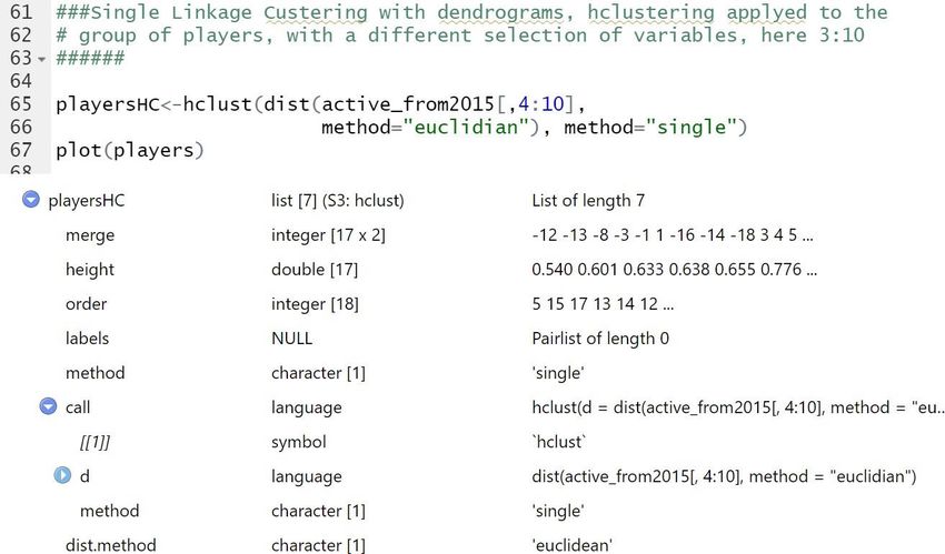
Figure 10 shows the flow chart of the algorithm. In this algorithm, the process ‘merge’ is
indicated. Every loop can make one or more merges in case of a tie. In Figure 11 an

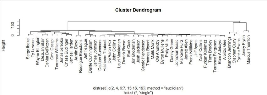
 29

example is shown. The code with hclust, method single and distance Euclidean is on top
of the figure. Below the code, the calculations and activity of the algorithm are shown in
the same figure. As a result, a dendrogram is drawn. Some examples of these dendrograms
come next chapter.

Figure 10: Flow chart of the Single Linkage algorithm (own elaboration)

Figure 11: Example of execution of the Single Linkage algorithm.

 30

 KMeans

 In clustering analysis, K-means is a well-known method. The goal is to solve the
 same problem than in Single Linkage but that here it is re-formulated taking into account
 the number of clusters that plays a special role because it will be part of the input. Given
 the data observations (or players, in this work)

 = { 1,· · · , }

The method seeks to minimize the function:

 ∑ ∑ 2( , ) ( . 2)
 =1 ∈ 

Over all possible observations q1, · · ·, qK.

 The method (see [22]) is based on building clusters trying to minimize the
 variance within the observations of the same group. That is, minimizing the within-cluster
 sum of squares over K clusters (Eq.2) is what the algorithm aims. However, this goal is
 an NP problem at it is said before and therefore, the algorithm described in [22] is just a
 heuristic. According to [23], the algorithm has strong consistency for clustering. This is
 the reason why it is very popular despite not guaranteeing the optimization goal or its
 convergence. The steps of the algorithm are as follows.

  Step 1: Initialization. The algorithm begins by partitioning the observation
 set into K random initial clusters. Also, this initialization can be done by
 using some heuristic device which improves the speed of the execution
 and quality of results especially when some information is known in
 advance.

  Step 2: The algorithm computes the cluster means.

  Step 3: The algorithm constructs a new partition by associating each point
 with the closest cluster mean. The latter yields new clusters.

  Step 4: Clustering comparison. If there are no changes, the process stops.
 If one or more observations change clusters, the process jumps to Step 2.

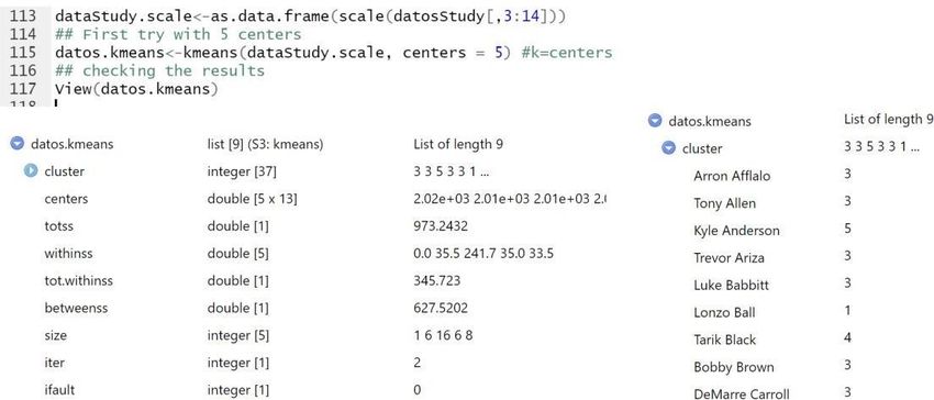
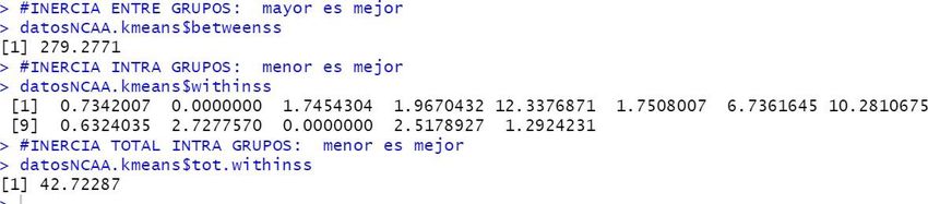
 31

Therefore, the algorithm works by making a new partition every step by
associating each observation with the closest cluster mean. These steps are repeated until
convergence. The number of clusters has no changes. Only the observations changes (or
not) the cluster where they belong. The stop occurs when the observations no longer
change clusters, the process converges.

 The algorithm works better when the variables are normalized, therefore, in the
first place, we have used the 'scale' function of R that allows this process to be carried out
easily on the variables chosen for the study. Next, we have made a loop to calculate the
values of the objective function (Eq.2 wich is equivalent to $tot.withinss in this model),
and thus determine the number K of clusters that we want to calculate. We have also
compared these values with those of the intra-group variance, given by the variable
$betweens. However, it is important to consider the variance within each group
individually, this is $withinss, which allows determining the homogeneity of each group.
To illustrate this, Figure 12 shows the output of an execution of Kmeans R function over
the same dataset example of players. In the top of the figure it is the code executed. The
line 113 of the code is a combination of the following actions: selection of the variables
(sequence 3:14 of the datosStudy dataset), normalization of the data with scale and
structure the result as data.frame mode. Line 115 instances the Kmeans algorithm for k=5
clusters (parameter ‘centers’). Line 115 produce the output below. In it, the structure of
the new object ‘datos.kmeans’ is shown. There are a total of 9 fields including $centers
(final centroid of each cluster), $withinss (list of the 5 within-cluster sum of squares),
$tot.withinss (the sum of the latter), $betweenss (intra-cluster sum of squares) , $size (list
of the 5 sizes of the clusters) and $iter (number of iterations of the algorithm). This
information is essential to analyze the quality of the results. On the right it is the list of
player’s names and the cluster they below.

 32

Figure 12. Data computed by the Kmeans algorithm

 To make a good choice of the number k, some authors recommend analyzing the
evolution of the variables $betweens and $tot.withinss. The first use to increase when the
number of clusters grows but from a certain value of K, the growth is negligible or just
decrease.
On the contrary, the variable tot.withinss decreases normally as the number of clusters
increases but it also can increase at a certain point or slow its decrease. The appropriate
K value is one where this variable starts to grow again or decreases very slowly. Figure
13 is an example of NBA 2009 dataset. The figure shows the evolution of these variables
in the execution of 11 instances of Kmeans algorithm. It can be seen how 7 can be an
adequate number of clusters according to these criteria.

Figure 13: Selection of an adequate K number of clusters for the NBA 2009 dataset

Once the clustering is done, it is easy to plot the results for a better visualization in reports
and helping with decision making. Next chapter contains some of these plots over the
specific datasets in the Draft study.

 33

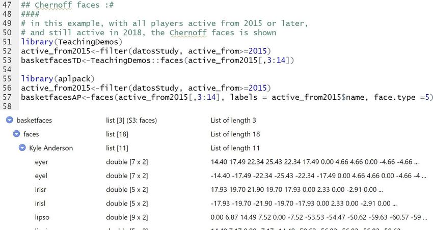
 Visualization with Chernoff faces

Chernoff faces is a method invented by Herman Chernoff [9] for easy classification of
multivariate data. The process consists of displaying multivariate data in the shape of a
human face. Each individual item within a face (eyes, ears, mouth, nose, chin and even a
hat of other elements if necessary) represents a value by different shapes and sizes. This
idea comes because face recognition is a natural way that humans can easily apply and
notice small changes without difficulty. The main use of face graphs was to enhance “the
user’s ability to detect and comprehend important phenomena” and to serve “as a
mnemonic device for remembering major conclusions” [9]. To draw the output faces, the
system handles each variable differently and can be fitted to facilitate the final
classification decision by choosing the features that are going to be mapped. In [11], for
example, the authors demonstrate that eye size and eyebrow-slant have been found to
carry significant weight.

 Recent applications of Chernoff faces include classification of drinking water
samples [10], graphical representation of multivariate data [11], experimental analysis
[12] and last year (2019) in cartography classification [13].

 TeachingDemos and AplPack libraries provide both the function ‘faces()’ that
makes the calculations of the distance matrix and the visualization of the resultant faces.
The AplPack function is more complete because also provide the characterization matrix
per each observation. Figure 14 shows an example of code where a set of players from
2015 is selected, and variables 3:14 are taken as input. The result output of distance is
shown below the code. For example, eye right (eyer) and eye left (eyel) of the player Kyle
Anderson have a list of numbers symmetric because they come from the same feature of
the player. Every item within the face is related in this way with a feature to draw it later,
as we show in the next chapter.

 34

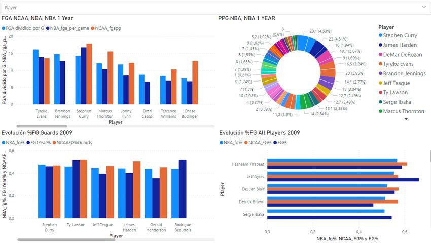
Figure 14: Example of Chernoff faces execution and the characterization matrix.

  Visualization with Power BI

The use of the Microsoft Power BI tool will offer us an overview of the different
relationships between both physical and game statistics of the players, which will allow
us to obtain conclusions about the behavior of these statistics. The main objective of
creating interactive visualizations is to be able to locate trends, and thus have a graphic
representation of the possible predictions resulting from this work. The first actions to be
carried out have to do with the arrangement and organization of the data. Making
decisions about what data to study and relating to obtain the best-performing graphs is
important. An example: it makes sense to relate two physical characteristics such as
weight and wingspan, but it does not make so much sense to relate age to a purely physical
characteristic. The main relationships that it has been decided to study are:

 ● Physical characteristics with position: players who can stand out in terms of
 physical characteristics over the rest of players of the same position are more
 likely to excel.

 ● Physical characteristics with shooting: In the historical records, a clear trend is
 noted that indicates that larger players have worse shooting percentages.

 ● Age with shooting percentages and number of shots: The evolution of the shot
 over time of the players will be studied.

 ● Shooting in NBA with shooting in NCAA: all statistics related to shooting will
 be studied to obtain the trends of change between leagues (professional and
 35

university)

● Draft classes with physical characteristics: This relationship allows us to know
the general election trends over the years exclusively by studying physical
characteristics.

 36

Chapter 5. Results

This chapter shows the results of the application of the clustering techniques developed
in this work, as well as the visualizations of the most remarkable results implemented in
RStudio and Power BI. To obtain the most representative results possible, a real case that
occurred in the NBA about a wrong choice in the order of the Draft players is exposed.
In the 2009 draft, the choices of each team had special relevance for their franchises,
given that they are considered one of the best generations of the Draft in recent years.
Stars like James Harden, Stephen Curry or Blake Griffin, were selected in this class of
the Draft. In this Draft class, bad predictions were given that marked the future of the
teams, by letting players leave who turned out to be better than the choice made. Stephen
Curry, Demar Derozan and Jrue Holiday were drafty underrated players by teams, but
they would end up being stars.

During the study, the behavior of the characteristics of these players, especially from
Stephen Curry, has been of vital importance.

The shooting of the players is an essential factor for the game of basketball, every attack
of a player revolves largely around his shot, and the study carried out has been based on
statistics and general shooting percentages. In this case, a study has been carried out around
the guards and guards belonging to the first round of said Draft. To access the data more
easily and efficiently, the results have been obtained by manipulating a dataset merged
between Seasons_Stats and Shooting_Stats. To complete the work, the results of the
application of the same methods are exposed to the players belonging to the most recent
Draft classes.

5.1 Clustering analytics results
This section shows the results of the clustering methods applied. We will present results
from both Single Linkage, as well as K-Means on selected sets of variables according to
the previous experience. The section includes also a critical comparison and explanation
of the charts.

  Single Linkage results

In the first place, the variables referring to percentages of field goals and free throws have
been selected. Besides, a distinction is made of the same type of variables in 3 different
 37

stages of the players: NBA career, First year in NBA, NCAA career. By applying
hierarchical clustering with the single method, specific dendrograms are created, referring

to the different percentages of each player, which indicate similarities between them. The
results are shown in Figures 15 and 16.

Figure 15: Dendrogram FT% on 3 features: Free Throw percentage in first season in NBA, NBA
career, NCAA career.

 38