The Queen's Gambit: Explaining the Superstar Effect Using Evidence from Chess
←
→
Page content transcription
If your browser does not render page correctly, please read the page content below
The Queen’s Gambit: Explaining the Superstar Effect
            Using Evidence from Chess *

                         Eren Bilen†         Alexander Matros†,‡

                                      March 7, 2021

Abstract. “Superstars” exist in many places – in classrooms, or in workplaces,
there is a small number of people who show extraordinary talent and ability. The
impact they have on their peers, however, is an ongoing research topic. In com-
petition, they might intimidate others; causing their peers to show less effort.
On the other hand, superstars might encourage higher effort, as their existence
in a competition encourages them to "step up" their game. In this study, we an-
alyze the impact of a superstar on their peers using evidence from chess. The
existence of a contemporary superstar (and the current World Chess Champion)
Magnus Carlsen, as well as, past world champions such as Garry Kasparov, Ana-
toly Karpov, or Bobby Fischer enables us to identify whether the existence of a
superstar in a chess tournament has a positive or an adverse effect on other
chess players’ performance. We identify errors committed by players using com-
puter evaluation that we run on our sample with 35,000 games and 2.8 million
moves with observations from 1962 to 2019, and estimate position complexity via
an Artificial Neural Network (ANN) algorithm that learns from an independent
sample with 25,000 games and 2 million moves. The results indicate that the
effect depends on the intensity of the superstar. If the skill gap between the su-
perstar and the rest of the competitors is large enough, an adverse effect exists.
However, when the skill gap is small, there may be slight positive peer effects.
In terms of head-to-head competition, the evidence shows that players commit
more mistakes against superstars in similarly-complex games. Understanding
the effect of superstars on peer performance is crucial for firms and managers
considering to introduce a superstar associate for their team.

JEL classification: M52, J3, J44, D3
Keywords: superstar, tournament, effort, chess

    * We would like to thank seminar participants at Dickinson College, Laboratory Innovation
Science at Harvard, Lancaster University, Murray State University, Sabanci University, South-
ern Illinois University Edwardsville, University of Nebraska Omaha, and University of South
Carolina, as well as, participants in the 6th Contests Theory and Evidence conference at the Uni-
versity of East Anglia and the 90th Southern Economic Association Meeting for their questions
and suggestions. We thank the Darla Moore School of Business Research Grant Program for the
financial support.
    † Department of Economics, University of South Carolina, Columbia, SC 29208. Email:

eren.bilen@grad.moore.sc.edu, alexander.matros@moore.sc.edu
    ‡ Department of Economics, Lancaster University, Lancaster, LA1 4YX, United Kingdom

Email: a.matros@lancaster.ac.uk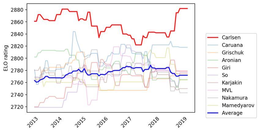
1. Introduction

                                                            "When you play against Bobby
                                                            [Fischer], it is not a question of
                                                            whether you win or lose. It is a
                                                            question of whether you survive."

                                                                  −Boris Spassky, World Chess
                                                                      Champion, 1969 - 1972.

Maximizing their employees’ efforts is one of the chief goals of the firm. To this
extent, firms typically encourage competition among their employees and allo-
cate bonuses according to their performance and effort. At the same time, firms
want to hire the best workers – preferably, the ones who are “superstars” in their
fields. For this reason, it is not unusual to see million-dollar hiring contracts
among the Forbes top 500 firms.
    However, hiring a superstar employee might potentially cause unintentional
side effects. Brown (2011) took a creative approach to analyze these potential
side effects by considering a famous golf superstar: Tiger Woods. Her goal was
to uncover whether Tiger Woods had a positive or negative effect on his competi-
tors’ performance. She compared performances in tournaments with and with-
out Tiger Woods and unveiled that there was a sharp decline in performance in
tournaments where Tiger Woods competed. This evidence points out that Tiger
Woods, as a superstar, creates a psychological pressure on his competitors which
has a discouraging effect, causing them to perform worse than their typical per-
formance.
    In this paper, we analyze the superstar effect using chess data.1 Chess pro-
vides a clean setting to analyze the superstar effect for the following reasons:
First, non-player related factors are minimal to non-existent in chess since every
chess board is the same for all players.2 Second, the move-level performance in-
dicators can be obtained with the use of computer algorithms that can evaluate
the quality of each move and estimate the complexity of each unique position.
   1 There is growing literature studying a broad range of questions using data from chess com-

petitions. For example, Levitt, List and Sadoff (2011) test whether chess masters are better at
making backward induction decisions. Gerdes and Gränsmark (2010) test for gender differences
in risk-taking using evidence from chess games played between male and female players, where
they find that women choose more risk-averse strategies playing against men. On the one hand,
Backus et al. (2016) and Smerdon et al. (2020) find that female players make more mistakes
playing against male opponents with similar strength. On the other hand, Stafford (2018) has
an opposite finding that women perform better against men with similar ELO ratings. Dreber,
Gerdes and Gränsmark (2013) test the relationship between attractiveness and risk-taking using
chess games.
   2 There is no compelling reason to expect a systematic difference in the environmental factors to

directly affect a tournament performance. However, Künn, Palacios and Pestel (2019) and Klingen
and van Ommeren (2020) find that indoor air quality has effects on performance and risk-taking
behavior of chess players.

                                                 2
Third, multiple chess superstars exist who lived in different time periods and
come from different backgrounds, enhancing the external validity of the study.3
    To begin with, we present a two-player contest model with a "superstar." Our
theory suggests that the skill gap between the superstar and the other player is
crucial to determine the superstar effect on the competition. If this gap is small,
then the superstar effect is positive: both players exert high effort. However,
when the skill gap is large, the superstar effect is negative: both players lower
their efforts. Our theory provides explanations for different superstar effects in
the literature. The negative superstar effect in golf is found not only in Brown
(2011), but also in Tanaka and Ishino (2012)4 , while the positive superstar effect
in track and field events is found in Hill (2014). He compares the performance
of athletes in runs where Usain Bolt is competing and where Usain Bolt is not
present, finding that athletes perform much better when Usain Bolt is compet-
ing. This can be attributed to non-superstar athletes being motivated by having
Usain Bolt running just “within their reach”, enabling them to push one step
further and show extra effort.
    Then, we test our theory on six different male and female chess superstars
who come from different backgrounds and time periods: Magnus Carlsen, Garry
Kasparov, Anatoly Karpov, Bobby Fischer, Hou Yifan, and Igors Rausis.5 We are
looking for direct (individual competition with a superstar) and indirect (perfor-
mance in a tournament with a superstar) superstar effects in chess tournaments.
To find these effects, we analyze 2.8 million move-level observations from elite
chess tournaments that took place between 1962 to 2019 with the world’s top
chess players. Our main performance indicator is unique to chess: the "Average
Centipawn Loss" (ACPL), which shows the amount of error a player commits in
a game.6 In chess, a player’s goal is to find the optimal move(s). Failing to do so
would result in mistake(s), which the ACPL metric captures. Having multiple
mistakes committed in a game almost certainly means losing at the top level
chess tournaments. We then test the following hypotheses:

   1. Direct effect: Do players commit more mistakes (than they are expected
      to) playing head-to-head against a superstar?

   2. Indirect effect: Do players commit more mistakes (than they are ex-
      pected to) in games played against each other if a superstar is present
      in the tournament as a competitor?

    Holding everything else constant, a player should be able to show the same
   3 In the media, "The Queen’s Gambit" gives a realistic portrayal of a chess superstar. The

protagonist, Beth Harmon, is a superstar who dominates her peers in tournaments. In this paper,
we analyze the real-life chess superstar effect on their peers in actual tournaments.
   4 Their superstar is Masashi Ozaki who competed in the Japan Golf Tour and dominated the

tournaments he participated in throughout the 1990s.
   5 We discuss why these players are superstars in Section 3.
   6 The Average Centipawn Loss is also referred to as "mean-error". We provide details on how

we use this metric in Section 3.4.

                                              3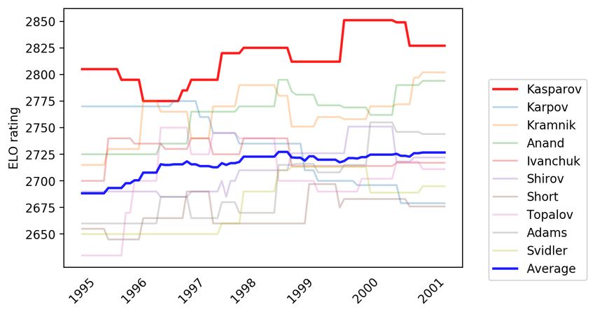
performance in finding the best moves in two "similarly complex" chess posi-
tions. The difficulty of finding the optimal moves − assuming players show full
effort − is related to two main factors: (1) External factors impacting a player.
For instance, being under pressure can lead the player to choke, resulting in
more mistakes. (2) The complexity of the position that the player faces. If both
players are willing to take risks, they can opt to keep more complex positions
on the board, which raises the likelihood that a player commits a mistake. To
isolate the "choking effect", we construct a complexity metric using a state-of-the
art Artificial Neural Network (ANN) algorithm that is trained with an indepen-
dent sample with more than 2 million moves.7 By controlling board complexity,
we compare games with identical difficulty levels. If a player commits more
mistakes against the superstar (or in the presence of a superstar) in similarly
complex games, it must be that either (i) the player chokes under pressure (that
is, even if the player shows full effort, the mental pressure of competing against
a superstar results in under-performance) or (ii) the player gives up and does not
show full effort, considering his or her ex-ante low winning chances (this results
in lower performance with more mistakes committed), or both (i) and (ii).
     We find a strong direct superstar effect: in similarly complex games, play-
ers commit more mistakes and perform below their expected level when they
compete head-to-head against the superstar. This result can be explained by
both the choking and the giving up effects. Consequently, players are less likely
to win and more likely to lose in these games compared to their games against
other opponents.
     We show that the indirect superstar effect depends on the skill gap be-
tween the superstar and the competition. As our theory predicts, we find that if
this gap is small, the indirect superstar effect is positive: it seems that the play-
ers believe they indeed have a chance to win the tournament and exert higher
effort. The data shows that the top 25 percent of the tournament participants
improve their performances and commit fewer mistakes. However, if the skill
gap is large, then the indirect superstar effect is negative: it seems that players
believe that their chances to win the tournament are slim, and/or that compet-
ing at the same tournament with a superstar creates psychological pressure. As
a result, the top players show an under-performance with more mistakes and
more losses. Interestingly, there is a tendency for the top players to play more
complex games in tournaments with a superstar. This suggests that the choking
effect is more dominant than the giving up effect.
     Our results provide clear takeaways for organizations: hiring a superstar
can have potential spillover effects, which could be positive for the whole organi-
zation if the superstar is slightly better than the rest of the group. However, the
organization can experience negative spillover effects if the skill gap between
the superstar and the rest of the group is substantial. Thus, managers should
compare the marginal benefit of hiring an "extreme" superstar to the potential
  7 The details of the algorithm are provided in Section 3.5.

                                                4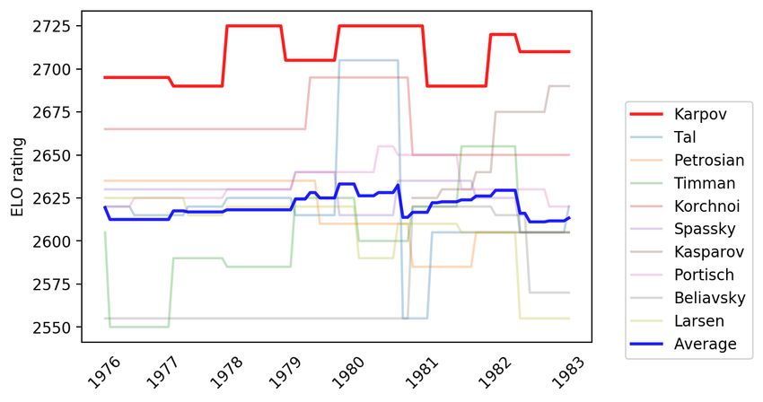
spillover costs on the whole organization.8 Moreover, hiring a marginally-better
superstar can act as a performance inducer for the rest of the team.
    The superstar literature started from Rosen (1981), who makes the first con-
tribution in the understanding of "superstars" by pointing out how skills in cer-
tain markets become excessively valuable. One of the most recent theoretical
contributions in the "superstar" literature is Xiao (2020), who demonstrates the
possibility of having positive or negative incentive effects when a superstar par-
ticipates in a tournament. These effects depend on the prize structure and the
participants’ abilities.
    Lazear and Rosen (1981), Green and Stokey (1983), Nalebuff and Stiglitz
(1983), and Moldovanu and Sela (2001) describe how to design optimal contracts
in rank-order tournaments. Prendergast (1999) provides a review on incentives
in workplaces.
    The empirical sports superstar literature started from Brown (2011)9 and is
ranging from professional track and field competitions to swimming. Yamane
and Hayashi (2015) compare the performance of swimmers who compete in ad-
jacent lanes and find that the performance of a swimmer is positively affected
by the performance of the swimmer in the adjacent lane. In addition, this effect
is amplified by the observability of the competitor’s performance. Specifically,
in backstroke competitions where observability of the adjacent lane is minimal,
there appears to be no effect, whereas the effect exists in freestyle competitions
with higher observability. Jane (2015) uses swimming competitions data in Tai-
wan and finds that having faster swimmers in a competition increases the over-
all performance of all the competitors participating in the competition.
    Topcoder and Kaggle are the two largest crowdsourcing platforms where con-
test organizers can run online contests offering prizes to contestants who score
the best in finding a solution to a difficult technical problem stated at the begin-
ning of the contest. Archak (2010) finds that players avoid competing against
superstars in Topcoder competitions. Studying the effect of increased competi-
tion on responses from the competitors, Boudreau, Lakhani and Menietti (2016)
discover that lower-ability competitors respond negatively to competition, while
higher-ability players respond positively. Zhang, Singh and Ghose (2019) suggest
that there may potentially be future benefits from competitions with superstars:
the competitors will learn from the superstar. This finding is similar to the pos-
   8 Mitigating the negative effects by avoiding within-organization pay-for-performance compen-

sation schemes is a possibility. However, it is challenging to eliminate all competition in an orga-
nization.
   9 Connolly and Rendleman (2014) and Babington, Goerg and Kitchens (2020) point out that an

adverse superstar effect may not be as strong as suggested by Brown (2011). They claim that
this result is not robust to alternative specifications and suggest that the effect could work in the
opposite direction – that the top competitors can perhaps bring forth the best in other players’
performance. In addition, Babington, Goerg and Kitchens (2020) provide further evidence using
observations from men’s and women’s FIS World Cup Alpine Skiing competitions and find little
to no peer effects when skiing superstars Hermann Maier and Lindsey Vonn participate in a
tournament. Our theory can suggest an explanation for these findings.

                                                 5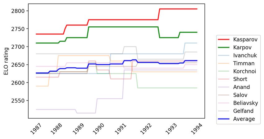
itive peer effects in the workplace and in the classroom, see Mas and Moretti
(2009), Duflo, Dupas and Kremer (2011), Cornelissen, Dustmann and Schönberg
(2017).
    The rest of the paper is organized as follows: Section 2 presents a two-player
tournament model with a superstar. Section 3 gives background information on
chess and describes how chess data is collected and analyzed. Section 4 provides
the empirical design. Section 5 presents the results, and section 6 concludes.

2. Theory
In this section, we consider a two-player contest in which player 1 competes
against a superstar, player 2.10 Player 1 maximizes his expected payoff, consist-
ing of expected benefits minus costly effort: 11
                                                  e1
                                  max                       V1 − e 1 ,
                                   e1        (e 1 + θ e 2 )
where e i is the effort of player i = 1, 2, V1 is a (monetary or rating/ranking) prize
which player 1 can win, and θ is the ability of player 2. We normalize the ability
of player 1 at one. Player 2, a superstar, has high ability θ ≥ 1 and maximizes
her expected payoff:

                                                 θ e2
                                  max                       V2 − e 2 ,
                                   e2        (e 1 + θ e 2 )
where V2 is the prize that player 2 can win. Note that θ is not only the ability of
player 2, but also the ratio of that player’s abilities.
   The first order conditions for players 1 and 2 are

                                         θ e2
                                                      V1 − 1 = 0,
                                    (e 1 + θ e 2 )2

and
                                         θ e1
                                                      V2 − 1 = 0.
                                    (e 1 + θ e 2 )2
Therefore, in an equilibrium
                                              e 2 V2
                                                 =   .
                                              e 1 V1
We can state our theoretical results now.

Proposition 1 Suppose that V1 > V2 . Then, there exists a unique equilibrium in
the two-player superstar contest model, where player i = 1, 2 exerts effort

                                               θ V1 V2
                                     e∗i =                 Vi .
                                             (V1 + θ V2 )2
 10 Tullock (1980) discussed a similar model, but did not provide a formal analysis.
 11 We assume that costs are linear functions.

                                                   6
In the equilibrium, player i = 1, 2 wins the contest with the probability p∗i , where
V1 θ V2
µ ¶
(p∗1 , p∗2 ) = , .
V1 + θ V2 V1 + θ V2
We assume that the prize for the underdog is greater than the prize for the
superstar in the two-player contest: everyone expects the superstar to win the
competition and her victory is neither surprising, nor too rewarding. However,
the underdog’s victory makes him special, which is also evident from rating point
calculations in chess: a lower rated player gains more rating points if he wins
against a higher ranked player.12 It follows from proposition 1 that the under-
dog, player 1, always exerts higher effort than the superstar, player 2, in the
equilibrium, since V1 > V2 . In addition, underdog’s winning chances decrease in
the superstar abilities. We have the following comparative statics results.
Proposition 2 Suppose that V1 > V2 . Then, individual equilibrium efforts in-
V1
crease in the superstar ability if θ ∗ < V2
and decrease if θ ∗ > V1
V2 .
V1
Individual equilibrium efforts are maximized if the superstar ability is θ ∗ = V2 .
Proposition 2 gives a unique value of the superstar ability which maximizes
individual and total equilibrium efforts. This observation suggests the best abil-
ity of a superstar for the contest designer.
Figure 1 illustrates this proposition and shows how equilibrium efforts and
winning probabilities change for different levels of superstar abilities if V1 =
10 and V2 = 4. When the ability ratio is small, effort levels for both players
increase. As the ability ratio increases, both players decrease their efforts. In
other words, if the gap between the superstar and the underdog abilities is small,
the superstar effect is positive as both players exert higher efforts. However, if
the superstar is much better than the underdog, then both players shirk in their
efforts and the superstar effect is negative.
12 The statement of Proposition 1 holds without the assumption about prizes. We will need this
assumption for the comparative statics results.
7Figure 1: Equilibrium effort and winning probabilities with prizes V1 = 10 and V2 = 4.
3. Data
3.1 Chess: Background
"It is an entire world of just 64
squares."
−Beth Harmon, The Queen’s
Gambit, Netflix Mini-Series (2020)
Chess is a two-player game with origins dating back to 6th century AD. Chess
is played over a 8x8 board with 16 pieces for each side (8 pawns, 2 knights, 2
bishops, 2 rooks, 1 queen, and 1 king). Figure 2 shows a chess board. Players
make moves in turns, and the player with the white pieces moves first. The
ultimate goal of the game is to capture the enemy king. A player can get close
to this goal by threatening the king through a "check": if the king has no escape,
the game ends with a "checkmate". A game can end in three ways: white player
wins, black player wins, or the game ends in a draw.
The possible combinations of moves in a chess game is estimated to be more
than the number of atoms in the universe.13 However, some moves are better
than others. With years of vigorous training, professional chess players learn
how to find the best moves by employing backward-induction and calculating
13 A lower bound on the number of possible moves is 10120 moves, per ? while the number of
atoms in the observable universe is estimated to be roughly 1080 .
88
rmblkans
7
opopopop
6
0Z0Z0Z0Z
5
Z0Z0Z0Z0
4
0Z0Z0Z0Z
3
Z0Z0Z0Z0
2
POPOPOPO
1
SNAQJBMR
a b c d e f g h
Figure 2: A chess board
consequences of moves to a certain complexity level. Failing to find the best
move(s) in a position would result in a "blunder" or a "mistake" which typically
leads to the player losing their game at the top level if a player commits multiple
blunders or mistakes. The player who performs better overall is the player who
manages to find the correct moves more often.
The standard measure of player strength in chess is the ELO rating system
first adopted by FIDE in 1970. This system was created by the Hungarian physi-
cist Arpad Elo (Elo 1978). Elo considers the performance of a player in a given
game as a random variable normally distributed around her unobservable true
ability. Each player gets a starting ELO rating which is updated according to
the outcome of each game via
£ ¡ ¢¤
ELO R,t+1 = ELO R,t + K S i − E t S i | R i , R j , (1)
where S i is the outcome of a game such that S i = 1 if player i wins the game,
S i = 0 if player i losses the game, and S i = 0.5 if the game ended in a draw.
¡ ¢
E t S i | R i , R j is the expected probability of player i winning the game given
the³ ELO ´ratings of the two players R i and R j which equals E (S R | R R , R B ) =
Φ R R400
−R B
where Φ(.) is the c.d.f. of the normal distribution.14 K is a parameter
for rate of adjustment.
This rating system allows comparisons of players’ strengths. For instance,
every month, FIDE publishes ELO ratings of all chess players. The Top 10
players are considered the most elite players in the world who earn significant
amounts of prizes and sponsorships. Moreover, chess titles have specific ELO
14 The probability that player i wins a game against player j is a function of their true abilities
³ x−[µ −µ ] ´ ³ 0−[µ −µ ] ´
[µ −µ ]
³ ´
P(p i > p j ) = P(p i − p j > 0) = 0∞ p 1 2 Φ pi j
= 1−Φ pi j
= Φ pR 2B , where p i is
R
2σ 2σ2 2σ2 2σ
the probability that player i with true ability µ i wins the game.
9rating requirements. For instance, the highest title in chess, Grandmaster, re-
quires the player to have an ELO rating 2500 or higher.15
Over the past decades, computer scientists have developed algorithms, or
"chess engines" that exploit the game-tree structure of chess. These engines
analyze each possible tree branch to come up with the best moves. The early
chess engines were inferior to humans. After a few decades, however, one chess
engine developed by IBM in the 1990s, Deep Blue, famously defeated the world
chess champion at the time, Garry Kasparov, in 1997. This was the first time
a world chess champion lost to a chess engine under tournament conditions.
Since then, chess engines have passed well beyond the human skills. As of 2021,
Stockfish 11 is the strongest chess engine with an ELO rating of 3497.16 In
comparison, the current world chess champion, Magnus Carlsen, has an ELO
rating of 2862.17
In addition to finding the best moves in a given position, a chess engine can
be used to analyze the games played between human players.18 The quality
of a move can be measured numerically by evaluating the move chosen by a
player and comparing it to the list of moves suggested by the chess engine. If
the move played by a player is considered a bad move by the engine, then that
move is assigned a negative value with its magnitude depending on the engine’s
evaluation.19
3.2 Chess Superstars
The first official world chess champion is Wilhelm Steinitz who won the title in
1886. Since Steinitz, there have been sixteen world chess champions in total.
Among these sixteen players, four have shown an extraordinary dominance over
their peers: Magnus Carlsen, Garry Kasparov, Anatoly Karpov, and Bobby Fis-
cher.20 We present evidence why these players were so dominant and considered
"superstars" in their eras. Specifically, we define a superstar as a player who
satisfies the following conditions: (i) be the world chess champion; (ii) win at
15 Our sample consists of the very elite chess players, often called "Super GMs", with ELO rat-
ings higher than 2700 in most cases.
16 Modern chess engines, such as Stockfish, have much higher ELO ratings compared to humans.
Most modern computers are strong enough to run Stockfish for analyzing chess positions and
finding the best moves, which is the engine we use in our analyses.
17 The highest ELO rating ever achieved by a human was 2882 in May 2014 by Magnus Carlsen.
18 Every chess game played at the top level is recorded, including all the moves played by the
players.
19 Engine evaluation scores in chess have no impact on the game outcomes. Engines are used in
post-game analysis for learning and research purposes. They are also used during live broadcast-
ing, such that the audience can see which player maintains an advantage. The use of a computer
engine by a player during a game is against fair play rules and is equivalent to using Performance
Enhancing Drugs (PEDs) for other sports.
20 In his classic series, "My Great Predecessors", Kasparov (2003) gives in-depth explanations
about his predecessors, outlining qualities of each world champion before him. In this paper, we
consider the "greatest of the greatest" world champions as "superstars" in their eras.
10least 50% of all tournaments participated in;21 (iii) maintain an ELO rating at
least 50 points above the average ELO rating of the world’s top 10 players (this
condition must hold for the post-1970 era when ELO rating was introduced); (iv)
have such a high ELO rating that just winning an elite tournament is not suf-
ficient to gain ELO rating points. We define an elite tournament, a tournament
which has (1) at least two players from the world’s Top 10 and (2) the average
ELO rating in the tournament is within 50 points of the average ELO rating in
tournaments with a superstar.
Magnus Carlsen is the current world chess champion, who first became cham-
pion in 2013 at age 22. He reached the highest ELO rating ever achieved in
history. Garry Kasparov was the world champion from 1985-2000 and was the
number one ranked chess player for 255 months, setting a record for maintain-
ing the number one position for the longest duration of time. For comparison,
Tiger Woods was the number one ranked player in the world for a total of 683
weeks, the longest ever in golf history. Anatoly Karpov was the world champion
before Kasparov in the years 1975-1985. He won over 160 tournaments, which is
a record for the highest number of tournaments won by a chess player.22 Bobby
Fischer was the world champion before Karpov between 1972 - 1975, winning all
U.S. championships he played in from 1957 (at age 14) to 1966. Fischer won the
1963 U.S. chess championship with a perfect 11 out of 11 score, a feat no other
player has ever achieved.23
In addition to the four male superstars, we consider a female chess super-
star: Hou Yifan, a four time women’s world chess champion between the years
2010-2017. She played three women’s world chess championship matches in this
period and did not lose a single game against her opponents, dominating the
tournaments from 2014 until she decided to stop playing in 2017.24
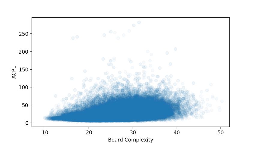
Figures 5–9 show how the four world chess champions: Carlsen, Kasparov,
21 For comparison, Tiger Woods won 24.2 percent of his PGA Tour events.
22 Kasparov (2003) shares an observation on Karpov’s effect on other players during a game in
Moscow in 1974: "Tal, who arrived in the auditorium at this moment, gives an interesting account:
"The first thing that struck me (I had not yet seen the position) was this: with measured steps
Karpov was calmly walking from one end of the stage to the other. His opponent was sitting with
his head in his hands, and simply physically it was felt that he was in trouble. ’Everything would
appear to be clear,’ I thought to myself, ’things are difficult for Polugayevsky.’ But the demonstration
board showed just the opposite! White was a clear exchange to the good − about such positions it
is customary to say that the rest is a matter of technique. Who knows, perhaps Karpov’s confidence,
his habit of retaining composure in the most desperate situations, was transmitted to his opponent
and made Polugayevsky excessively nervous." p. 239 "My Great Predecessors" Vol 5.
23 Kasparov (2003) on Fischer’s performance in 1963 U.S. championship: "Bobby crushed every-
one in turn, Reshevsky, Steinmeyer, Addison, Weinstein, Donald Byrne... Could no one really with-
stand him?! In an interview Evans merely spread his hands: ’Fantastic, unbelievable...’ Fischer
created around himself such an energy field, such an atmosphere of tension, a colossal psychologi-
cal intensity, that this affected everyone." See p. 310 "My Great Predecessors" Vol 4.
24 Not losing a single game in world championship matches is a very rare phenomenon since the
world champion and the contestant are expected to be at similar levels.
11Karpov and Hou Yifan performed compared to their peers across years.25 The
ELO rating difference between each superstar and the average of world’s top 10
players in each corresponding era is about 100 points. This rating gap is very
significant, especially at top-level competitive chess. For instance, the expected
win probabilities between two players with a gap of 100 ELO rating points are
approximately 64%-36%.
Figures 10–14 show individual tournament performances across years for
each superstar with the vertical axis showing whether the superstar gained or
lost rating points at the end of a tournament. For instance in 2001, Kasparov
played in four tournaments and won all of them. In one of these tournaments, he
even lost rating points despite winning. For the world’s strongest player, winning
a tournament is not sufficient to maintain or gain rating points because he also
has to win decisively.
We also consider a chess grandmaster, Igors Rausis, who competed against
non-masters in the years between 2012-2019. He was in the top 100 chess play-
ers in the world and played against players about 500 ELO rating points below
his rating. The ELO rating difference between him and his average opponent
in the tournaments is similar to the rating difference between the current world
champion Magnus Carlsen, with ELO rating of 2882, and the chess computer
program Stockfish 11, with ELO rating 3497. Figure 15 illustrates an example
of the ELO rating distribution of Rausis’ opponents in a tournament. His par-
ticipation in such tournaments created a unique setting where a strong chess
grandmaster plays against much lower rated non-master opponents. Obviously,
Rausis was a superstar in these tournaments.26
Table 1 presents statistics of the superstars’ dominance. Panels A-E include
the World’s Top 10 chess players for the corresponding era and a summary of
their tournament performances. For example, Magnus Carlsen participated in
35 tournaments with classical time controls between 2013 and 2019, winning
21 of them. This 60% tournament win rate is two times higher than World’s #2
chess player, Fabiano Caruana, who has a tournament win rate of 30%. A more
extreme case is Anatoly Karpov, who won 26 out of 32 tournaments, which con-
verts to an 81% tournament win rate while the runner up Jan Timman had a
tournament win rate of 22%.27 The final panel, panel F, shows the tournament
performances for Rausis and his top-performing opponents. Rausis showed an
outstanding performance by winning all eight tournaments in the sample with-
out facing a single loss.
25 ELO rating information is not available for Fischer’s era. FIDE adopted the ELO rating sys-
tem in 1970.
26 Igors Rausis was banned by FIDE, the International Chess Federation, in July 2019 due to
cheating by using a chess engine on his phone during tournaments.
27 Restricting the runner-ups’ tournament wins to tournaments in which a superstar partici-
pated lowers their tournament win rate significantly. Tables are available upon request.
12Table 1: World’s Top 10 chess players and their tournament performances
years: 2013-2019 PANEL A
# of tournament # of tournaments % tournament proportion of proportion of proportion of # of # of
Name ELO ACPL complexity
wins played wins games won draws games lost moves games
Carlsen, Magnus 21 35 60% 2855 0.352 0.576 0.072 14.413 26.802 16,104 303
Caruana, Fabiano 15 49 30% 2802 0.283 0.592 0.126 16.758 28.280 22,205 447
So, Wesley 6 27 22% 2777 0.226 0.666 0.108 14.928 25.717 11,622 263
Aronian, Levon 5 33 15% 2788 0.196 0.662 0.142 16.059 25.654 13,455 294
Giri, Anish 3 31 9% 2770 0.149 0.719 0.131 14.873 26.202 14,224 304
Karjakin, Sergey 3 28 10% 2768 0.168 0.689 0.143 15.947 26.938 12,764 281
Mamedyarov, Shakhriyar 3 22 13% 2777 0.172 0.674 0.154 15.050 26.339 9,405 216
Nakamura, Hikaru 3 35 8% 2779 0.218 0.622 0.160 15.823 27.398 15,349 327
Vachier Lagrave, Maxime 3 26 11% 2777 0.163 0.703 0.134 14.539 26.842 10,227 232
Grischuk, Alexander 0 15 0% 2777 0.183 0.633 0.184 18.081 27.539 6,852 146
years: 1995-2001 PANEL B
# of tournament # of tournaments % tournament proportion of proportion of proportion of # of # of
Name ELO ACPL complexity
wins played wins games won draws games lost moves games
Kasparov, Garry 17 22 77% 2816 0.439 0.510 0.051 17.595 28.509 18,082 488
Kramnik, Vladimir 12 30 40% 2760 0.322 0.621 0.058 16.743 26.071 22,782 610
Anand, Viswanathan 9 25 36% 2762 0.305 0.595 0.099 19.337 28.328 18,879 517
Topalov, Veselin 6 26 23% 2708 0.279 0.514 0.207 21.193 22,081 28.801 515
Ivanchuk, Vassily 4 17 23% 2727 0.255 0.582 0.164 19.626 27.045 13,673 362
Adams, Michael 3 22 13% 2693 0.255 0.575 0.169 19.096 27.382 17,472 421
Short, Nigel D 3 18 16% 2673 0.272 0.475 0.253 22.717 29.080 13,538 348
Svidler, Peter 3 13 23% 2684 0.234 0.599 0.167 19.340 27.573 9,458 260
Karpov, Anatoly 2 12 16% 2742 0.214 0.679 0.107 18.292 26.457 8,966 211
Shirov, Alexei 2 26 7% 2706 0.288 0.460 0.253 21.865 29.014 22,277 529Table 1 (cont): World’s Top 10 chess players and their tournament performances
years: 1976-1983 PANEL C
# of tournament # of tournaments % tournament proportion of proportion of proportion of # of # of
Name ELO ACPL complexity
wins played wins games won draws games lost moves games
Karpov, Anatoly 26 32 81% 2707 0.432 0.524 0.044 17.429 25.244 14,581 391
Timman, Jan H 7 32 21% 2607 0.333 0.525 0.142 20.777 26.074 17,690 305
Larsen, Bent 5 27 18% 2607 0.383 0.342 0.274 23.726 27.251 17,495 193
Kasparov, Garry 3 5 60% 2652 0.429 0.487 0.084 20.459 25.634 2,207 53
Portisch, Lajos 3 20 15% 2634 0.324 0.516 0.160 20.471 25.729 10,744 204
Tal, Mihail 3 11 27% 2632 0.271 0.652 0.077 19.898 24.915 5,505 131
Petrosian, Tigran V 2 12 16% 2608 0.244 0.652 0.103 20.810 23.089 5,257 100
Spassky, Boris Vasilievich 2 16 12% 2624 0.196 0.697 0.107 19.789 24.771 6,115 157
Beliavsky, Alexander G 1 5 20% 2596 0.320 0.457 0.223 23.923 28.210 2,758 58
Kortschnoj, Viktor Lvovich 1 2 50% 2672 0.558 0.292 0.150 22.860 28.550 1,106 23
years: 1962-1970 PANEL D
# of tournament # of tournaments % tournament proportion of proportion of proportion of # of # of
Name ELO ACPL complexity
wins played wins games won draws games lost moves games
Fischer, Robert James 12 16 75% . 0.641 0.286 0.073 18.405 28.622 10,706 252
Kortschnoj, Viktor Lvovich 7 12 58% . 0.469 0.459 0.072 19.964 26.378 7,728 197
Keres, Paul 4 8 50% . 0.420 0.547 0.032 19.080 25.084 4,830 139
Spassky, Boris Vasilievich 4 9 44% . 0.410 0.570 0.020 18.240 24.341 4,365 138
Botvinnik, Mikhail 3 5 60% . 0.529 0.414 0.056 18.769 26.065 2,251 63
Geller, Efim P 2 12 16% . 0.425 0.506 0.069 18.519 25.024 8,432 220
Tal, Mihail 2 8 25% . 0.466 0.402 0.133 21.894 26.928 4,615 123
Petrosian, Tigran V 1 13 7% . 0.334 0.621 0.045 20.311 24.675 7,622 227
Reshevsky, Samuel H 1 11 9% . 0.258 0.505 0.237 24.871 25.505 5,253 140
Bronstein, David Ionovich 0 6 0% . 0.283 0.628 0.089 21.604 25.199 3,043 94Table 1 (cont): World’s Top 10 chess players and their tournament performances
years: 2014-2019 PANEL E
# of tournament # of tournaments % tournament proportion of proportion of proportion of # of # of
Name ELO ACPL complexity
wins played wins games won draws games lost moves games
Hou, Yifan 4 4 100% 2644 0.614 0.364 0.023 16.222 26.820 4,028 88
Ju, Wenjun 3 6 50% 2563 0.400 0.523 0.077 16.565 26.079 5,826 130
Koneru, Humpy 2 6 33% 2584 0.379 0.424 0.197 20.033 27.516 5,832 132
Dzagnidze, Nana 0 6 0% 2540 0.359 0.347 0.295 24.728 28.335 6,080 128
Goryachkina, Aleksandra 0 1 0% 2564 0.364 0.636 0.000 14.322 27.547 1,116 22
Kosteniuk, Alexandra 0 7 0% 2532 0.297 0.508 0.195 22.841 29.092 6,878 150
Lagno, Kateryna 0 2 0% 2544 0.227 0.682 0.091 16.283 26.304 1,666 44
Muzychuk, Anna 0 5 0% 2554 0.218 0.582 0.200 18.416 26.901 4,814 110
Muzychuk, Mariya 0 3 0% 2544 0.242 0.576 0.182 18.302 27.178 3,056 66
Zhao, Xue 0 6 0% 2519 0.288 0.424 0.288 24.058 27.521 5,990 132
years: 2012-2019 PANEL F*
# of tournament # of tournaments % tournament proportion of proportion of proportion of # of # of
Name ELO ACPL complexity
wins played wins games won draws games lost moves games
Rausis, Igors 8 8 100% 2578 0.783 0.217 0.000 18.319 25.436 3,864 105
Naumkin, Igor 1 4 25% 2444 0.667 0.228 0.106 24.891 26.162 1,746 48
Patuzzo, Fabrizio 1 3 33% 2318 0.600 0.133 0.267 28.208 26.425 1,322 25
Reinhardt, Bernd 1 4 25% 2207 0.423 0.215 0.362 32.870 27.644 1,299 27
Bardone, Lorenzo 0 3 0% 2095 0.433 0.267 0.300 27.199 26.779 890 24
Gascon del Nogal, Jose R 0 2 0% 2469 0.625 0.250 0.125 23.560 28.387 1,162 32
Lubbe, Melanie 0 4 0% 2316 0.401 0.263 0.336 25.243 25.287 1,730 40
Lubbe, Nikolas 0 4 0% 2467 0.527 0.442 0.031 24.480 25.623 1,676 48
Luciani, Valerio 0 4 0% 2158 0.485 0.083 0.432 35.437 27.656 1,352 35
Montilli, Vincenzo 0 3 0% 2117 0.311 0.422 0.267 32.871 26.972 1,278 26
Notes: Panels A-E show the tournament performance for the World’s Top 10 chess players for the corresponding time period. ELO rating was first
adopted by the International Chess Federation (FIDE) in 1970, hence this information is absent in Panel D for Fischer’s sample. Variables and their
definitions are presented in table Table A.1.
∗ : Panel F shows the tournament performance for Rausis and his top performing opponents.3.3 ChessBase Mega Database
Our data comes from the 2020 ChessBase Mega Database containing over 8 mil-
lion chess games dating back to the 1400s. Every chess game is contained in a
PGN file which includes information about player names, player sides (White or
Black), ELO ratings, date and location of the game, tournament name, round,
and the moves played. An example of a PGN file and a tournament table is
provided in the appendix. See Table A.2 and Figure A.1.
Table A.1 in the appendix provides a summary of variables used and their
definitions. Table 2 presents the summary statistics for each era with tourna-
ments grouped according to the superstar presence. In total, our study analyzes
over 2 million moves from approximately 35,000 games played in over 300 tour-
naments between 1962 and 2019.28
3.4 Measuring Performance
3.4.1 Average Centipawn Loss
Our first metric comes from computer evaluations where we identify mistakes
committed by each player in a given game.29 A chess game g consists of moves
m ∈ {1, . . . , M } where player i makes an individual move m i g . A chess engine can
evaluate a given position by calculating layers with depth n at each decision node
and make suggestions about the best moves to play. Given a best move is played,
computer
the engine provides the relative (dis)advantage in a given position C i gm .
pla yer
This evaluation is then compared to the actual evaluation score C i gm once a
player makes his or her move. The difference in scores reached via the engine’s
top suggested move(s) and the actual move a player makes can be captured by
¯ ¯
¯ computer pla yer ¯
error i gm = ¯C i gm − C i gm ¯ . (2)
If the player makes a top suggested move, the player has committed zero error,
computer pla yer
i.e., C i gm = C i gm . We can think of chess as a game of attrition where
the player who makes less mistakes eventually wins the game. While staying
constant if top moves are played, the evaluation shows an advantage for the
opponent if a player commits a mistake by playing a bad move.
We then take the average of all the mistakes committed by player i in game
g via
P M ¯¯ computer ¯
pla yer ¯
m=1 ¯ C i gm
− C i gm ¯
error i g = , (3)
M
which is a widely accepted metric named Average Centipawn Loss (ACPL). ACPL
is the average of all the penalties a player is assigned by the chess engine for the
28 A list of the tournaments is provided in the appendix.
29 Guid and Bratko (2011) and Regan, Biswas and Zhou (2014) are two early examples of imple-
mentations of computer evaluations in chess.
16mistakes they committed in a game. If the player plays the best moves in a
game, his ACPL score will be small where a smaller number implies the player
performed better. On the other hand, if the player makes moves that are consid-
ered bad by the engine, the player’s ACPL score would be higher.
We used Stockfish 11 in our analysis with depth n = 19 moves. For each move,
computer
the engine was given half a second to analyze the position and assess |C i gm −
pla yer
C i gm |. Figure 16 shows an example of how a game was analyzed. For instance,
at move 30, the computer evaluation is +3.2, which means that the white player
has the advantage by a score of 3.2: roughly the equivalent of being one piece
(knight or bishop) up compared to his opponent. If the white player comes up
with the best moves throughout the rest of the game, the evaluation can also
stay 3.2 (if the black player also makes perfect moves) or only go up leading to
a possible win toward the end of the game. In the actual game, the player with
the white pieces lost his advantage by making bad moves and eventually lost the
game. The engine analyzes all 162 moves played in the game and evaluates the
quality of each move. Dividing the sum of mistakes committed by player i to the
total number of moves played by player i gives the player-specific ACPL score.
3.4.2 Board Complexity
Our second measure that reinforces our ACPL metric is "board complexity" which
we obtain via an Artificial Neural Network (ANN) approach. The recent de-
velopments with AlphaGo and AlphaZero demonstrated the strength of using
heuristic-based algorithms that perform at least as good as the traditional ap-
proaches, if not better.30 Instead of learning from self-play, our neural-network
algorithm "learns" from human players.31 To train the network, we use an in-
dependent sample published as part of a Kaggle contest consisting of 25,000
games and more than 2 million moves, with Stockfish evaluation included for
each move.32 The average player in this sample has an ELO rating of 2280,
which corresponds to the "National Master" level according to the United States
Chess Federation (USCF).33
The goal of the network is to predict the probability of a player making a
mistake with its magnitude. This task would be trivial to solve for positions that
were previously played. However, each chess game reaches a unique position
after the opening stage which requires accurate extrapolation of human play in
30 https://en.chessbase.com/post/leela-chess-zero-alphazero-for-the-pc
31 Sabatelli et al. (2018) and McIlroy-Young et al. (2020) are two recent implementations of such
architecture.
32 https://www.kaggle.com/c/finding-elo/data
33 http://www.uschess.org/index.php/Learn-About-Chess/FAQ-Starting-Out.html
17Bias
b
z1 w1
Activation
function Output
Inputs z2 w2
Σ f y
z3 w3
Weights
Figure 3: Example of a simple perceptron, with 3 input units (each with its unique weight) and
1 output unit.
order to predict the errors.34 We represent a chess position through the use of
its 12 binary features, corresponding to the 12 unique pieces on the board (6 for
White, 6 for Black). A chess board has 8 × 8 = 64 squares. We split the board
into 12 separate 8 × 8 boards (one for each piece) where a square gets "1" if the
piece is present on that particular square and gets "0" otherwise. In total, we
represent a given position using 12 × 8 × 8 = 768 inputs. We add one additional
feature to represent the players’ turn (white to move, or black to move) and thus
have 768 + 1 = 769 inputs in total per position. Figure 4 illustrates. 35
The neural network "learns" from 25,000 games by observing each of the ap-
proximately two million positions and estimates the optimal weights by minimiz-
ing the error rate that results from each possible set of weights with the Gradient
Descent algorithm. The set of 1,356,612 optimal weights uniquely characterizes
our network. We use two networks to make a prediction on two statistics for a
given position: (i) probability that a player commits an error and (ii) the amount
of error measured in centipawns. For a full game, the two statistics multiplied
(and averaged out across moves) gives us an estimate for the ACPL that each
player is expected to get as the result of the complexity of the game
XM ³¯
¯ computer
¯ ´¯
¯ computer
¯
network ¯ network ¯
m=1
P ¯ C i gm
− C i gm ¯ > 0 ¯ C i gm
− C i gm ¯
E(error i g ) = , (4)
M
34 This approach is vastly different than traditional analysis with an engine such as Stockfish.
Engines are very strong and can find the best moves. However, they cannot give any informa-
tion about how a human would play in a given situation because they are designed to find the
best moves without any human characteristics. Our neural-network algorithm is specifically de-
signed to learn how and when humans make mistakes in given positions from analyzing mistakes
committed by humans from a sample of 2 million moves.
35 We use a network architecture with three layers. Figure 3 illustrates. The layers have 1048,
500, and 50 neurons, each with its unique weight. In order to prevent overfitting, a 20% dropout
regularization on each layer is used. Each hidden layer is connected with the Rectified Linear
Unit (ReLU) activation function. The Adam optimizer was used with a learning rate of 0.001.
181st hidden layer kth hidden layer
input layer
y1(1) ... y1(k)
z1
output layer
y2(1) y2(k)
z2 ... y1(k+1)
.. ..
. .
..
.
zN ...
(1) ( k)
ym (1) ym ( k)
Figure 4: Network graph of a multilayer neural network with (k + 1) layers, N input units, and 1
output unit. Each neuron collects unique weights from each previous unit. The kth hidden layer
contains m(k) neurons.
¯ ¯
¯ computer
where ¯C i gm − C network ¯ is the expected centipawn loss in a given position
¯
i gm
predicted by the neural network. We test our network’s performance on our main
"superstars" sample.36 The mean ACPL for the whole sample with 35,000 games
is 25.87, and our board complexity measure, which is the expected ACPL that
we obtained through our network, is 26.56.37 Figure 19 shows a scatterplot of
ACPL and the expected ACPL. The slope coefficient is 1.14, which implies that
a point increase in our complexity measure results in a 1.14 point increase in
the actual ACPL score.38 Figure 20 shows the distributions of ACPL and the
expected ACPL.
The board complexity measure addresses the main drawback of using only
ACPL scores. The ACPL score of a player is a function of his or her opponent’s
strength and their strategic choices. For instance, if both players find it optimal
to not take any risks, they can have a simple game where players make little
to no mistakes, resulting in low ACPL scores. Yet, this would not imply that
players showed a great performance compared to their other −potentially more
complex− games. Being able to control for complexity of a game enables us to
36 Figures 17–18 show our network’s prediction on a game played by Magnus Carlsen.
37 The reason why our network −which was trained with games played at on average 2280 ELO
level− makes a close estimate for the ACPL in the main sample is that the estimates come from
not a single player with ELO rating 2280, but rather from a "committee" of players with ELO
rating 2280 on average. Hence the network is slightly "stronger" compared to an actual 2280
player.
38 The highest ACPL prediction of the network is 50.2 while about 8% of the sample has an
actual ACPL > 50.2. These extreme ACPL cases are under-predicted by the network due to the
network’s behavior as a "committee" rather than a single player, where the idiosyncratic shocks
are averaged out.
19compare mistakes committed in similarly-complex games.
3.4.2 Game outcomes
The third measure we use is game-level outcomes. Every chess game ends in
a win, a loss, or a draw. The player who wins a tournament is the one who
accumulates more wins and fewer losses, as the winner of a game receives a full
point toward his or her tournament score.39 In other words, a player who has
more wins in a tournament shows a higher performance. In terms of losses, the
opposite is true. If a player has many losses in a tournament, their chances to
win the tournament are slim. Of course, a draw is considered better than a loss
and worse than a win.
4. Empirical Design
Our baseline model compares a player’s performance in a tournament where a
superstar is present with their performance in a tournament without a super-
star. This can be captured by the following equation:
P er f ormance i, j = β0 +β1 Su perstar j × H i ghELO i, j +β2 Su perstar j × M idELO i, j
+ β3 Su perstar j × LowELO i, j + β4 H i ghELO i, j + β5 M idELO i, j
+ Θ X i, j + η i + ² i, j , (5)
where P er f ormance i, j is the performance of player i in tournament j, measured
by methods discussed in section 3.4. Su perstar j is an indicator for a superstar
being present in tournament j. ² i, j is an idiosyncratic shock. Having negative
signs for coefficients β1 , β2 , and β3 means that the superstar presence creates an
adverse effect: players are discouraged to demonstrate their best efforts result-
ing in worse performance outcomes. H i ghELO i, j equals one if the player has an
ELO rating within the top quartile in the ELO rating distribution of the tour-
nament participants. M idELO i, j captures the second and third quartiles, and
LowELO i, j captures the bottom quartile. Θ X i, j contains the game and tourna-
ment level controls. In addition to tournament level specifications, chess allows
for a game level analysis which can be specified as the following:
P er f ormance i, j,k = α0 + α1 A gainstSu perstar i, j,k + Φ X i, j + η i + ² i, j,k , (6)
where A gainstSu perstar i, j,k equals one if player i in tournament j plays against
a superstar in round k. In this specification, α1 captures the effect of head-to-
head competition against a superstar.
39 A draw brings half a point, while a loss brings no points in a tournament.
20Note that chess superstars as a rule play in the strongest tournaments,
which guarantees more money and higher prestige. However, it is not possi-
ble to play in all top-level tournaments.40 Typically, if a player competes in a
world championship match in a given year, (s)he tends to play in fewer tourna-
ments in that particular year to be able to prepare for the world championship
match.41 In years without a world championship match, the world champion
typically picks a certain number of tournaments to participate in. (S)he may
play in fewer tournaments if (s)he believes that the schedule does not allow for
adequate preparation for each tournament. We control for the average ELO rat-
ing in a tournament to account for any selection issues.42
5. Results
Table 3 shows the performance of non-superstar players playing against a su-
perstar for each sample. There is a distinct pattern that is true for all super-
stars: playing against them is associated with a higher ACPL score, more blun-
ders, more mistakes, lower chances to win, and higher chances to lose. What
is more, games played against superstars are more complex. This higher com-
plexity could be due to the superstar’s willingness to reach more complex posi-
tions in order to make the ability-gap more salient. It could also be linked to
a non-superstar player taking more risk.43 Taken as a whole, players commit
more blunders and mistakes, holding board complexity constant. For instance, a
player who plays against Fischer shows an ACPL that is 4.3 points higher com-
pared to his games against other players with a similar complexity level. His
likelihood is 10 percentage points less for a win, 18 percentage points less for a
draw, and 29 percentage points higher for a loss compared to his typical games.
This implies that in terms of direct competition, these superstars have a strong
dominance over their peers. Rausis, unsurprisingly, and Hou Yifan, surprisingly,
show the strongest domination, with Fischer closely following in third position
40 In our sample with elite tournaments, a tournament with a superstar has, on average, an
average ELO score that is 50 points higher compared to the tournaments without a superstar.
This shows that chess superstars indeed play in the strongest tournaments.
41 We indeed document a negative correlation between the number of tournaments a superstar
plays and world championship years. These results are available upon request.
42 Linnemer and Visser (2016) document self-selection in chess tournaments with stronger play-
ers being more likely to play in tournaments with higher prizes. A central difference between
their sample and ours is the level of tournaments, with their data coming from the World Open
tournament, which is an open tournament with non-master participants with Elo ratings between
1400-2200. Meanwhile, our sample consists of players from a much more restricted sample with
only the most elite Grandmasters having Elo ratings often above 2700. Moreover, these high-level
tournaments are invitation based; i.e., tournament organizers offer invitations to a select group
of strong players, with these restrictions working against any possible selection issues.
43 It is not a trivial task to identify which player initiates complexity. Typically, complex games
are reached with mutual agreement by players, avoiding exchanges and keeping the tension on
the board.
21behind these two players. The magnitudes for ACPL, win, and loss probabilities
are stronger for these players compared to the rest of the samples.44
Tables 4–12 show the effect of a superstar’s presence on the performance of
other competitors. Rausis, the most dominant superstar according to Table 3,
has a negative effect on the top players’ performances.45 However, focusing on
the last three rounds − the rounds where the winner is determined by the Swiss
pairing format − a large adverse effect exists for the top players. These players
have an ACPL score that is 2.4 points higher, about 65% higher chances of com-
mitting a blunder, and 23% less chances of winning.46 A similar adverse effect
on the top players is true for the second most dominant superstar, Hou Yifan.
Her presence is associated with an ACPL score that is 4.5 points higher, 11%
less chances of winning, and 17% higher chances of losing for the top players in
a tournament. For Fischer, the coefficients for ACPL, blunders, and mistakes
are positive but imprecise. Fischer’s opponents indeed had more draws and less
complex-games, which agrees with the findings in Moul and Nye (2009) on Soviet
collusion.
Another situation with intense competition is when two superstars, Kas-
parov and Karpov, both participate in a tournament. This means that for a
given player, he or she will have to face both Kasparov and Karpov and perform
better than both of them in order to win the tournament. This tough competition
appears to lead to more decisive games and less draws, with players committing
fewer blunders and mistakes. The top quartile of players, who usually try to
compete with Kasparov and Karpov, experience a lot of pressure and as a result,
increased losses. However, these players also win more games.47
Players perform better if they face only Kasparov or Karpov in the tourna-
ment compared to facing both superstars in the tournament. With one superstar,
either Kasparov or Karpov, in the tournament, players have higher chances of
winning the tournament and as a result, play more accurately and manage to
get more wins, with substantial gains in the ACPL score and less mistakes com-
mitted. This improvement is the strongest for the top quartile of players.
Surprisingly, Carlsen is the least dominant superstar in our sample because
his presence appears to create a slight positive effect on performance. Players
play more accurately and make fewer mistakes under higher challenges with
more complex positions. The positive effect appears to apply to all the tourna-
44 Taken as a whole, these findings verify that the superstars considered in our study indeed
show greater performance compared to their peers.
45 Unsurprisingly, Rausis’ effect on all participants is minimal. The average number of partic-
ipants in an open Swiss-format tournament is typically more than fifty with very heterogeneous
participants.
46 The top players perform better at the beginning of a tournament with Rausis, and their mo-
tivation appears to vanish toward the end of the tournament when critical games for the tourna-
ment victory are decided. We focus on the latter results due to higher stakes in the final rounds.
47 In fact, the bottom quartile of players shows better performance with Kasparov and Karpov’s
presence. These players have more wins and fewer losses as a result of a worse performance by
the upper quartile.
22You can also read