NflWAR: A Reproducible Method for Offensive Player Evaluation in Football
←
→
Page content transcription
If your browser does not render page correctly, please read the page content below
nflWAR: A Reproducible Method for Offensive
                                                      Player Evaluation in Football
                                                           (Extended Edition)
                                                       Ronald Yurko, Samuel Ventura, and Maksim Horowitz
arXiv:1802.00998v2 [stat.AP] 12 Jul 2018

                                                 Department of Statistics & Data Science, Carnegie Mellon University
                                                                                       July 13, 2018

                                                                                            Abstract
                                                    Unlike other major professional sports, American football lacks comprehensive statisti-
                                                cal ratings for player evaluation that are both reproducible and easily interpretable in terms
                                                of game outcomes. Existing methods for player evaluation in football depend heavily on pro-
                                                prietary data, are not reproducible, and lag behind those of other major sports. We present
                                                four contributions to the study of football statistics in order to address these issues. First, we
                                                develop the R package nflscrapR to provide easy access to publicly available play-by-play
                                                data from the National Football League (NFL) dating back to 2009. Second, we introduce
                                                a novel multinomial logistic regression approach for estimating the expected points for each
                                                play. Third, we use the expected points as input into a generalized additive model for esti-
                                                mating the win probability for each play. Fourth, we introduce our nflWAR framework, using
                                                multilevel models to isolate the contributions of individual offensive skill players, and provid-
                                                ing estimates for their individual wins above replacement (WAR). We estimate the uncertainty
                                                in each player’s WAR through a resampling approach specifically designed for football, and
                                                we present these results for the 2017 NFL season. We discuss how our reproducible WAR
                                                framework, built entirely on publicly available data, can be easily extended to estimate WAR
                                                for players at any position, provided that researchers have access to data specifying which
                                                players are on the field during each play. Finally, we discuss the potential implications of this
                                                work for NFL teams.

                                           Keywords: multilevel model, generalized additive model, multinomial logistic regression, R,
                                           reproducibility

                                                                                                1
1     Introduction
Despite the sport’s popularity in the United States, public statistical analysis of American football
(“football”) has lagged behind that of other major sports. While new statistical research involving
player and team evaluation is regularly published in baseball (Albert, 2006; Jensen et al., 2009;
Piette and Jensen, 2012; Baumer et al., 2015), basketball (Kubatko et al., 2007; Deshpande and
Jensen, 2016), and hockey (Macdonald, 2011; Gramacy et al., 2012; Thomas et al., 2013), there
is limited new research that addresses on-field or player personnel decisions for National Football
League (NFL) teams. Recent work in football addresses topics such as fantasy football (Becker
and Sun, 2016), predicting game outcomes (Balreira et al., 2014), NFL TV ratings (Grimshaw
and Burwell, 2014), the effect of “fan passion” and league sponsorship on brand recognition
(Wakefield and Rivers, 2012), and realignment in college football (Jensen and Turner, 2014).
Additionally, with the notable exception of Lock and Nettleton (2014), recent research relating to
on-field or player personnel decisions in football is narrowly focused. For example, Mulholland
and Jensen (2014) analyze the success of tight ends in the NFL draft, Clark et al. (2013) and
Pasteur and Cunningham-Rhoads (2014) both provide improved metrics for kicker evaluation,
Martin et al. (2017) examine the NFL’s change in overtime rules, and Snyder and Lopez (2015)
focus on discretionary penalties from referees. Moreover, statistical analysis of football that
does tackle on-field or player personnel decisions frequently relies on proprietary and costly data
sources, where data quality often depends on potentially biased and publicly unverified human
judgment. This leads to a lack of reproducibility that is well-documented in sports research
(Baumer et al., 2015).
     In this paper, we posit that (1) objective on-field and player personnel decisions rely on two
fundamental categories of statistical analysis in football: play evaluation and player evaluation,
and (2) in order to maintain a standard of objectivity and reproducibility for these two fundamen-
tal areas of analysis, researchers must agree on a dataset standard.

1.1    Previous Work: Evaluating Plays
The most basic unit of analysis in football is a single play. In order to objectively evaluate on-field
decisions and player performance, each play in a football game must be assigned an appropriate
value indicating its success or failure. Traditionally, yards gained/lost have been used to evaluate
the success of a play. However, this point of view strips away the importance of context in
football (Carter and Machol, 1971; Carroll et al., 1988). For instance, three yards gained on 3rd
and 2 are more valuable than three yards gained on 3rd and 7. This key point, that not all yards
are created equal, has been the foundation for the development of two approaches for evaluating
plays: expected points and win probability. The expected points framework uses historical data
to find the number of points eventually scored by teams in similar situations, while the win
probability framework uses historical data to find how often teams in similar situations win the
game. Using these metrics, one can obtain pre-snap and post-snap values of a play (expected
points or win probability) and, taking the difference in these values, the value provided by the play
itself – expected points added (EPA) or win probability added (WPA). These approaches have
been recently popularized by Brian Burke’s work at www.advancedfootballanalytics.com
and ESPN (Burke, 2009; Katz and Burke, 2017).

                                                  2
Most of the best known approaches for calculating expected points do not provide any level
of statistical detail describing their methodology. In most written descriptions, factors such as
the down, yards to go for a first down, and field position are taken into account. However, there
is no universal standard for which factors should be considered. Carter and Machol (1971) and
others essentially use a form of “nearest neighbors” algorithms (Dasarathy, 1991) to identify
similar situations based on down, yards to go, and the yard line to then average over the next
points scored. Goldner (2017) describes a Markov model and uses the absorption probabilities
for different scoring events (touchdown, field goal, and safety) to arrive at the expected points for
a play. ESPN has a proprietary expected points metric, but does not detail the specifics of how
it is calculated (Pattani, 2012). Burke (2009) provides an intuitive explanation for what expected
points means, but does not go into the details of the calculations. Schatz (2003) provides a
metric called “defense-adjusted value over average”, which is similar to expected points, and also
accounts for the strength of the opposing defense. However, specifics on the modeling techniques
are not disclosed. Causey (2015) takes an exact-neighbors approach, finding all plays with a set
of identical characteristics, taking the average outcome, and conducting post-hoc smoothing to
calculate expected points. In this work, Causey explores the uncertainty in estimates of expected
points using bootstrap resampling and analyzes the changes in expected point values over time.
Causey also provides all code used for this analysis.
     Depending on how metrics based on expected points are used, potential problems arise when
building an expected points model involving the nature of football games. The main issue, as
pointed out by Burke (2014), involves the score differential in a game. When a team is leading
by a large number of points at the end of a game, they will sacrifice scoring points for letting time
run off the clock. Changes in team behavior in these situations and, more generally, the leverage
of a play in terms of its potential effect on winning and losing are not taken into account when
computing expected points.
     Analyzing changes in win probability for play evaluation partially resolves these issues. Com-
pared to expected points models, there is considerably more literature on different methodologies
for estimating the win probability of a play in football. Goldner (2017) uses a Markov model,
similar to the approach taken by Tango, Lichtman, and Dolphin (2007) in baseball, by including
the score differential, time remaining, and timeouts to extend the expected points model. Burke’s
approach is primarily empirical estimation by binning plays with adjustments and smoothing.
In some published win probability analyses, random forests have been shown to generate well-
calibrated win probability estimates (Causey, 2013; Lock and Nettleton, 2014). The approach
taken by Lock and Nettleton (2014) also considers the respective strengths of the offensive (pos-
session) and defensive (non-possession) teams.
     There are many areas of research that build off of these approaches for valuing plays. For
example, analyses of fourth down attempts and play-calling are very popular (Romer, 2006;
Alamar, 2010; Goldner, 2012; Quealy et al., 2017). This paper focuses on using play evaluation
to subsequently evaluate players, and we discuss prior attempts at player evaluation below.

1.2    Previous Work: Evaluating Players
Due to the complex nature of the sport and the limited data available publicly, the NFL lacks com-
prehensive statistics for evaluating player performance. While there has been extensive research

                                                 3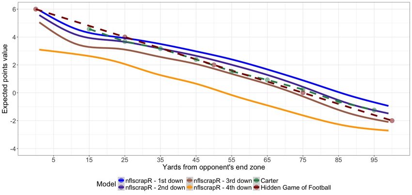
on situational analysis and play evaluation as described above, there has been considerably less
focus on player evaluation. Existing measures do not accurately reflect a player’s value to NFL
teams, and they are not interpretable in terms of game outcomes (e.g. points or wins). Similarly,
there are no publicly known attempts for developing a Wins Above Replacement (WAR) measure
for every individual NFL player, as made popular in baseball (Schoenfield, 2012) and other sports
(Thomas and Ventura, 2015).
    Previous methods for player evaluation in football can be broken down into three categories:
within-position statistical comparisons, ad hoc across-position statistical comparisons, and across-
position statistical comparisons that rely on proprietary data or human judgment.

1.2.1   Within-Position Player Evaluation
Approaches for quantitatively evaluating players who play the same position are numerous, vary
by position, and typically lag behind those of other sports. For comparisons of players at of-
fensive skill positions such as quarterback (QB), running back (RB), wide receiver (WR), and
tight end (TE), most analysis relies on basic box score statistics. These include yards gained via
passing, rushing, and/or receiving; touchdowns via passing, rushing, and/or receiving; rushing
attempts for RBs; receptions and targets for RBs, WRs, and TEs; completions, attempts, comple-
tion percentage, and yard per attempt for QBs; and other similar derivations of simple box score
statistics. These metrics do not account for game situation or leverage. Additionally, they only
provide an estimate of a player’s relative value to other players at the same position. We cannot
draw meaningful conclusions about cross-positional comparisons.
    Linear combinations of these box score statistics, such as passer rating (Smith et al., 1973),
are often used to compare players at the same position while taking into account more than just
a single box score measure. Similarly, Pro Football Reference’s adjusted net yards per attempt
(“ANY/A”) expands upon passer rating in that it accounts for sacks and uses a different linear
weighting scheme (Pro-Football-Reference, 2018). These metrics involve outdated and/or ad hoc
weights, thresholds, and other features. Passing in the NFL has changed substantially since the
conception of the passer rating statistic in 1973, so that the chosen weights and thresholds do not
have the same meaning in today’s game as they did in 1973. While ANY/A accounts for sacks
and uses a different weighting system, it is hardly a complete measure of QB performance, since
it does not account for game situation and leverage. Perhaps most importantly, both passer rating
and ANY/A are not interpretable in terms of game outcomes like points or wins.
    For positions other than QB, RB, WR, and TE, data is limited, since the NFL does not pub-
licly provide information about which players are on the field for a particular play, the offensive
and defensive formations (other than the “shotgun” formation on offense), or the pre- and post-
snap locations of players on the field. For offensive linemen, very little information is available
to statistically compare players, as offensive linemen typically only touch the football on bro-
ken plays. For defensive players, the NFL only provides information about which players were
directly involved in a play (e.g. the tackler or the defensive back covering a targeted receiver).
As such, with these positions, it is difficult to obtain adequate within-positional comparisons of
player value, let alone across-position comparisons.

                                                 4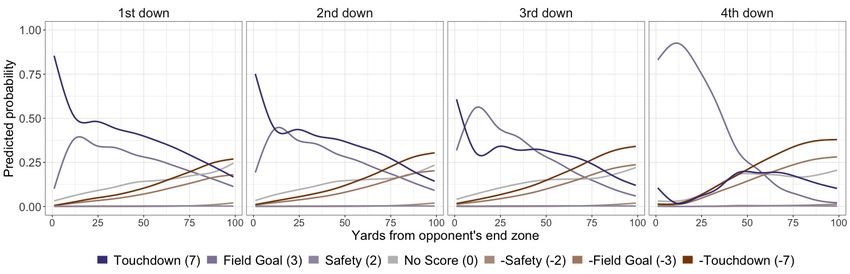
1.2.2   Ad Hoc Across-Position Player Evaluation
Using only box score statistics, it is extremely difficult to ascertain the value of players at differ-
ent positions. The fantasy sports industry has attempted to provide across-position estimates of
player value using box score statistics. These estimates typically use ad hoc linear combinations
of box score statistics that differ by position, so as to put the in-game statistical performances
of players at different positions on comparable scales. These measures, typically referred to as
“fantasy points”, are available for all positions except those on the offensive line.
    Of course, these metrics have several issues. First, they involve many unjustified or ad hoc
weights. For example, one rushing yard is worth about 40% of one passing yard in ESPN’s
standard definitions of these metrics (ESPN, 2017), but these relative values are arbitrary. Second,
the definitions are inconsistent, with different on-field events having different values for players
of different positions. For example, defensive interceptions are typically worth three times as
much as quarterback interceptions thrown (Ratcliffe, 2013; ESPN, 2017). Third, these measures
do not account for context, such as the game situation or the leverage of a given play. Finally,
they are not directly interpretable in terms of game outcomes (e.g. points or wins).

1.2.3   Player Evaluation with Proprietary Data or Human Judgment
Outside of the public sphere, there have been irreproducible attempts at within-position statis-
tical comparisons of NFL players. Pro Football Focus assigns grades to every player in each
play, but this approach is solely based on human judgment and proprietary to PFF (Eager et al.,
2017). ESPN’s total quarterback rating (“QBR”) accounts for the situational contexts a QB faces
throughout a game (Katz and Burke, 2017; Oliver, 2011). ESPN uses the following approach
when computing QBR: First, they determine the degree of success or failure for each play. Sec-
ond, they divide credit for each play amongst all players involved. Third, additional adjustments
are made for plays of very little consequence to the game outcome. This approach has several
important advantages. In the first step, the EPA is used to assign an objective value to each play.
Another advantage is that some attempt is made to divide credit for a play’s success or failure
amongst the players involved. In the approach for NFL player evaluation we propose in this
paper, we loosely follow these same two steps.
    ESPN’s QBR has some disadvantages, however. First and most importantly, Total QBR is
not directly reproducible, since it relies on human judgment when evaluating plays. “The details
of every play (air yards, drops, pressures, etc.) are charted by a team of trained analysts in the
ESPN Stats & Information Group. Every play of every game is tracked by at least two different
analysts to provide the most accurate representation of how each play occurred” (Katz and Burke,
2017). Additionally, while QBR down-weights plays in low-leverage situations, the approach for
doing so is not clearly described and appears to be ad hoc. Finally, QBR is limited only to the
QB position.
    The only public approach for evaluating players at all positions according to common scale is
Pro Football Reference’s “approximate value” (AV) statistic (Drinen, 2013). Using a combination
of objective and subjective analysis, AV attempts to assign a single numerical value to a player’s
performance in any season since 1950, regardless of the player’s position. AV has some subjective
components, such as whether or not a lineman was named to the NFL’s “all-pro” team, and
whether a running back reaches the arbitrary threshold of 200 carries. Additionally, since AV

                                                  5
uses linear combinations of end-of-season box score statistics to evaluate players, it does not take
into account game situation, opponent, or many other contextual factors that may play a role in
the accumulation of box score statistics over the course of a season. Finally, although the basis
of many AV calculations involves points scored and allowed, AV is not interpretable in terms of
game outcomes.

1.3    Our Framework for Evaluating NFL Plays and Players
In order to properly evaluate players, we need to allocate a portion of a play’s value to each
player involved (Katz and Burke, 2017). Baumer and Badian-Pessot (2017) details the long
history of division of credit modeling as a primary driver of research in sports analytics, with
origins in evaluating run contributions in baseball. However, in comparison to baseball, every
football play is more complex and interdependent, with the 22 players on the field contributing
in many ways and to varying degrees. A running play depends not only on the running back but
the blocking by the linemen, the quarterback’s handoff, the defensive matchup, the play call, etc.
A natural approach is to use a regression-based method, with indicators for each player on the
field for a play, providing an estimate of their marginal effect. This type of modeling has become
common in basketball and hockey, because it accounts for factors such as quality of teammates
and competition (Rosenbaum, 2004; Kubatko et al., 2007; Macdonald, 2011; Gramacy et al.,
2012; Thomas et al., 2013).
    We present four contributions to the study of football statistics in order to address the issues
pertaining to play evaluation and player evaluation outlined above:

   1. The R package nflscrapR to provide easy access to publicly available NFL play-by-play
      data (Section 2).

   2. A novel approach for estimating expected points using a multinomial logistic regression
      model, which more appropriately models the “next score” response variable (Section 3.1).

   3. A generalized additive model for estimating the win probability using the expected points
      as input (Section 3.2).

   4. Our nflWAR framework, using multilevel models to isolate offensive skill player contribu-
      tion and estimate their WAR (Section 4).

    We use a sampling procedure similar to Baumer et al. (2015) to estimate uncertainty in each
player’s seasonal WAR. Due to the limitations of publicly available data, the primary focus of this
paper is on offensive skill position players: QB, RB, WR, and TE. However, we present a novel
metric that serves as a proxy for measuring a team’s offensive line performance on rushing plays.
Furthermore, the reproducible framework we introduce in this paper can also be easily extended
to estimate WAR for all positions given the appropriate data. Researchers with data detailing
which players are on the field for every play can use the framework provided in Section 6.4 to
estimate WAR for players at all positions.
    Our WAR framework has several key advantages. First, it is fully reproducible: it is built
using only public data, with all code provided and all data accessible to the public. Second,
our expected points and win probability models are well-calibrated and more appropriate from

                                                 6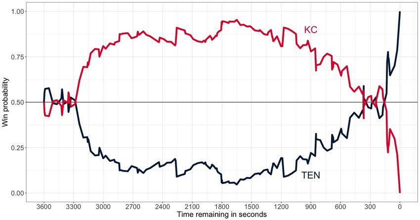
a statistical perspective than other approaches. Third, player evaluation with WAR is easily in-
terpretable in terms of game outcomes, unlike prior approaches to player evaluation in the NFL
discussed above. The replacement level baseline informs us how many wins a player adds over
a readily available player. This is more desirable than comparing to average from the viewpoint
of an NFL front office, as league average performance is still valuable in context (Baumer et al.,
2015). Fourth, the multilevel model framework accounts for quality of teammates and compe-
tition. Fifth, although this paper presents WAR using our expected points and win probability
models for play evaluation, researchers can freely substitute their own approaches for play eval-
uation without any changes to the framework for estimating player WAR. Finally, we recognize
the limitations of point estimates for player evaluation and provide estimates of the uncertainty
in a player’s WAR.

2    Play-by-Play Data with nflscrapR
Data in professional sports comes in many different forms. At the season-level, player and team
statistics are typically available dating back to the 1800s (Lahman, 1996 – 2017, Phillips (2018)).
At the game-level, player and team statistics have been tracked to varying degrees of detail dating
back several decades (Lahman, 1996 – 2017). Within games, data is available to varying degrees
of granularity across sports and leagues. For example, Major League Baseball (MLB) has play-
by-play data at the plate appearance level available dating back several decades (Lahman, 1996
– 2017), while the National Hockey League (NHL) only began releasing play-by-play via their
real-time scoring system in the 2005-06 season (Thomas and Ventura, 2017).
    Play-by-play data, or information specifying the conditions, features, and results of an indi-
vidual play, serves as the basis for most modern sports analysis in the public sphere (Kubatko
et al., 2007, Macdonald (2011), Lock and Nettleton (2014), Thomas and Ventura (2017)). Out-
side of the public sphere, many professional sports teams and leagues have access to data at even
finer levels of granularity, e.g. via optical player tracking systems in the National Basketball As-
sociation, MLB, and the English Premier League that track the spatial distribution of players and
objects at multiple times per second. The NFL in 2016 began using radio-frequency identification
(RFID) technology to track the locations of players and the football (Skiver, 2017), but as of mid
2018, this data is not available publicly, and NFL teams have only just gained accessed to the
data beyond their own players. In almost all major professional sports leagues, play-by-play data
is provided and includes information on in-game events, players involved, and (usually) which
players are actively participating in the game for each event (Thomas and Ventura, 2017, Lahman
(1996 – 2017)).
    Importantly, this is not the case for the NFL. While play-by-play data is available through
the NFL.com application programming interface (API), the league does not provide information
about which players are present on the playing field for each play, what formations are being
used (aside from the “shotgun” formation), player locations, or pre-snap player movement. This
is extremely important, as it limits the set of players for which we can provide estimates of their
contribution to game outcomes (e.g. points scored, points allowed, wins, losses, etc).
    We develop an R package (R Core Team, 2017), called nflscrapR, that provides users with
clean datasets, box score statistics, and more advanced metrics describing every NFL play since

                                                 7
2009 (Horowitz et al., 2017). This package was inspired largely by other R packages facilitating
the access of sports data. For hockey, nhlscrapR provides clean datasets and advanced metrics to
use for analysis for NHL fans (Thomas and Ventura, 2017). In baseball, the R packages pitchRx
(Sievert, 2015), Lahman (Lahman, 1996 – 2017), and openWAR (Baumer et al., 2015) provide tools
for collecting MLB data on the pitch-by-pitch level and building out advanced player evaluation
metrics. In basketball, ballR (Elmore and DeWitt, 2017) provides functions for collecting data
from basketball-reference.com.
    Each NFL game since 2009 has a 10 digit game identification number (ID) and an associated
set of webpages that includes information on the scoring events, play-by-play, game results, and
other game data. The API structures its data using JavaScript Object Notation (JSON) into three
major groups: game outcomes, player statistics at the game level, and play-by-play information.
The design of the nflscrapR package closely mimics the structure of the JSON data in the API,
with four main functions described below:
    season games(): Using the data structure outputting end of game scores and team matchups,
this function provides end of game results with an associated game ID and the home and away
teams abbreviations.
    player game(): Accessing the player statistics object in the API’s JSON data, this function
parses the player level game summary data and creates a box-score-like data frame. Additional
functions provide aggregation functionality:
season player game() binds the results of player game() for all games in a season, and
agg player season() outputs a single row for each player with their season total statistics.
    game play by play(): This is the most important function in nflscrapR. The function
parses the listed play-by-play data then uses advanced regular expressions and other data ma-
nipulation tasks to extract detailed information about each play (e.g. players involved in ac-
tion, play type, penalty information, air yards gained, yards gained after the catch, etc.). The
season play by play() binds the results of game play by play() for all games in a season.
    season rosters(): This function outputs all of the rostered players on a specified team in
a specified season and includes their name, position, unique player ID, and other information.
    For visualization purposes we also made a dataset, nflteams available in the package which
includes the full name of all 32 NFL teams, their team abbreviations, and their primary colors1 .
    In addition to the functions provided in nflscrapR, we provide downloadable versions in
comma-separated-value format, along with a complete and frequently updating data dictionary,
at https://github.com/ryurko/nflscrapR-data. The datasets provided on this website in-
cluded play-by-play from 2009 – 2017, game-by-game player level statistics, player-season total
statistics, and team-season total statistics. These datasets are made available to allow users fa-
miliar with other software to do research in the realm of football analytics. Table 1 gives a brief
overview of some of the more important variables used for evaluating plays in Section 3.
  1 Some   of this information is provided through Ben Baumer’s R package teamcolors (Baumer and Matthews,
2017)

                                                    8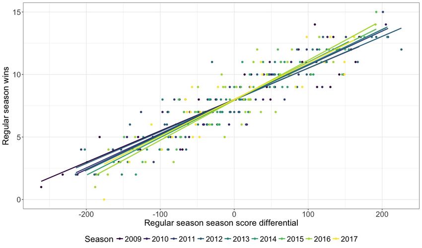
Table 1: Description of the play-by-play dataset.
            Variable             Description

            Possession Team      Team with the ball on offense (opposing team is on
                                 defense)
            Down                 Four downs to advance the ball ten (or more) yards
            Yards to go          Distance in yards to advance and convert first down
            Yard line            Distance in yards away from opponent’s endzone
                                 (100 to zero)
            Time Remaining       Seconds remaining in game, each game is 3600 sec-
                                 onds long (four quarters, halftime, and a potential
                                 overtime)
            Score differential   Difference in score between the possession team and
                                 opposition

3       Evaluating Plays with Expected Points and Win Probability
As described in Section 1.1, expected points and win probability are two common approaches for
evaluating plays. These approaches have several key advantages: They can be calculated using
only data provided by the NFL and available publicly, they provide estimates of a play’s value in
terms of real game outcomes (i.e. points and wins), and, as a result, they are easy to understand
for both experts and non-experts.
    Below, we introduce our own novel approaches for estimating expected points (EP) and win
probability (W P) using publicly available data via nflscrapR.

3.1     Expected Points
While most authors take the average “next score” outcome of similar plays in order to arrive at an
estimate of EP, we recognize that certain scoring events become more or less likely in different
situations. As such, we propose modeling the probability for each of the scoring events directly,
as this more appropriately accounts for the differing relationships between the covariates in Table
1 and the different categories of the “next score” response. Once we have the probabilities of each
scoring event, we can trivially estimate expected points.

3.1.1    Multinomial Logistic Regression
To estimate the probabilities of each possible scoring event conditional on the current game sit-
uation, we use multinomial logistic regression. For each play, we find the next scoring event
within the same half (with respect to the possession team) as one of the seven possible events:
touchdown (7 points), field goal (3 points), safety (2 points), no score (0 points), opponent safety
(-2 points), opponent field goal (-3 points), and opponent touchdown (-7 points). Here, we ignore

                                                 9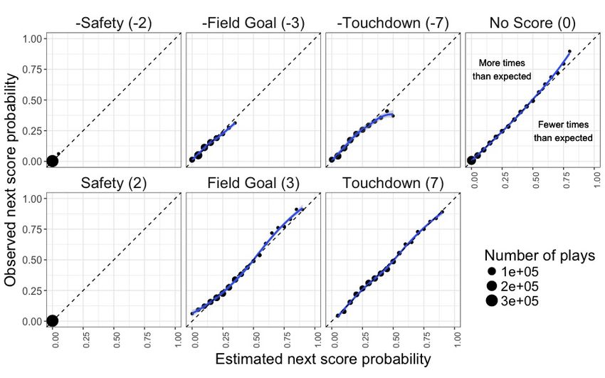
Table 2: Description of variables for the EP model.
           Variable             Variable description

           Down                 The current down (1st, 2nd, 3rd, or 4th
           Seconds              Number of seconds remaining in half
           Yardline             Yards from endzone (0 to 100)
           log(YTG)             Log transformation of yards to go for a first down
           GTG                  Indicator for whether or not it is a goal down situation
           UTM                  Indicator for whether or not time remaining in the half
                                is under two minutes

point after touchdown (PAT) attempts, and we treat PATs separately in Section 3.1.4.
    Figure 1 displays the distribution of the different type of scoring events using data from
NFL regular season games between 2009 and 2016, with each event located on the y-axis based
on their associated point value y. This data consists of 304,896 non-PAT plays, excluding QB
kneels (which are solely used to run out the clock and are thus assigned an EP value of zero).
The gaps along the y-axis between the different scoring events reinforce our decision to treat
this as a classification problem rather than modeling the point values with linear regression –
residuals in such a model will not meet the assumptions of normality. While we use seven points
for a touchdown for simplicity here, our multinomial logistic regression model generates the
probabilities for the events agnostic of the point value. This is beneficial, since it allows us to
flexibly handle PATs and two-point attempts separately. We can easily adjust the point values
associated with touchdowns to reflect changes in the league’s scoring environment.

Figure 1: Distribution of next scoring events for all plays from 2009-16, with respect to the
possession team.

                                                10
We denote the covariates describing the game situation for each play as X, which are pre-
sented in Table 2, and the response variable:
Y ∈{Touchdown (7), Field Goal (3), Safety (2), No Score (0),
− Touchdown (-7), −Field Goal (-3), −Safety (-2)} (1)
The model is specified with six logit transformations relative to the “No Score” event with
the following form:
P(Y = Touchdown|X)
log( ) = X · β Touchdown ,
P(Y = No Score|X)
P(Y = Field Goal|X)
log( ) = X · β Field Goal ,
P(Y = No Score|X)
..
. (2)
P(Y = −Touchdown|X)
log( ) = X · β −Touchdown ,
P(Y = No Score|X)
where β y is the corresponding coefficient vector for the type of next scoring event. Using the
generated probabilities for each of the possible scoring events, P(Y = y|X), we simply calculate
the expected points (EP) for a play by multiplying each event’s predicted probability with its
associated point value y:
EP = E[Y |X] = ∑ y · P(Y = y|X). (3)
y
3.1.2 Observation Weighting
Potential problems arise when building an expected points model because of the nature of football
games. The first issue, as pointed out by Burke (2014), regards the score differential in a game.
When a team is leading by a large number of points at the end of a game they will sacrifice scoring
points for letting time run off the clock. This means that plays with large score differentials can
exhibit a different kind of relationship with the next points scored than plays with tight score
differentials. Although others such as Burke only use the subset of plays in the first and third
quarter where the score differential is within ten points, we don’t exclude any observations but
instead use a weighting approach. Figure 2(a) displays the distribution for the absolute score
differential, which is clearly skewed right, with a higher proportion of plays possessing smaller
score differentials. Each play i ∈ {1, . . . , n}, in the modeling data of regular season games from
2009 to 2016, is assigned a weight wi based on the score differential S scaled from zero to one
with the following function:
max(|Si |) − |Si |
i
wi = w(Si ) = . (4)
max(|Si |) − min(|Si |)
i i
In addition to score differential, we also weight plays according to their “distance” to the next
score in terms of the number of drives. For each play i, we find the difference in the number of
11drives from the next score D: Di = dnext score − di , where dnext score and di are the drive numbers
for the next score and play i, respectively. For plays in the first half, we stipulate that Di = 0 if the
dnext score occurs in the second half, and similarly for second half plays for which the next score is
in overtime. Figure 2(b) displays the distribution of Di excluding plays with the next score as “No
Score.” This difference is then scaled from zero to one in the same way as the score differential in
Equation 4. The score differential and drive score difference weights are then added together and
again rescaled from zero to one in the same manner resulting in a combined weighting scheme.
By combining the two weights, we are placing equal emphasis on both the score differential and
the number of drives until the next score and leave adjusting this balance for future work.
Figure 2: Distributions for (a) absolute score differential and (b) number of drives until next score
(excluding plays without a next score event).
3.1.3 Model Selection with Calibration
Since our expected points model uses the probabilities for each scoring event from multino-
mial logistic regression, the variables and interactions selected for the model are determined via
calibration testing, similar to the criteria for evaluating the win probability model in Lock and
Nettleton (2014). The estimated probability for each of the seven scoring events is binned in five
percent increments (20 total possible bins), with the observed proportion of the event found in
each bin. If the actual proportion of the event is similar to the bin’s estimated probability then
the model is well-calibrated. Because we are generating probabilities for seven events, we want
a model that is well-calibrated across all seven events. To objectively compare different models,
we first calculate for scoring event y in bin b ∈ {1, . . . , B} its associated error ey,b :
ey,b = |P̂b (Y = y) − Pb (Y = y)|, (5)
where P̂b (Y = y) and Pb (Y = y) are the predicted and observed probabilities, respectively, in bin
b. Then, the overall calibration error ey for scoring event y is found by averaging ey,b over all
bins, weighted by the number of plays in each bin, ny,b :
1
ey = ny,b · ey,b , (6)
ny ∑
b
12where ny = ∑b ny,b . This leads to the model’s calibration error e as the average of the seven ey
values, weighted by the number of plays with scoring event y, ny :
1
e= ny · ey , (7)
n∑y
where n = ∑y ny , the number of total plays. This provides us with a single statistic with which to
evaluate models, in addition to the calibration charts.
We calculate the model calibration error using leave-one-season-out cross-validation (LOSO
CV) to reflect how the nflscrapR package will generate the probabilities for plays in a season it
has not yet observed. The model yielding the best LOSO CV calibration results uses the variables
presented in Table 2, along with three interactions: log(YTG) and Down, Yardline and Down, and
log(YTG) and GTG. Figure 3 displays the selected model’s LOSO CV calibration results for each
of the seven scoring events, resulting in e ≈ 0.013. The dashed lines along the diagonal represent
a perfect fit, i.e. the closer to the diagonal points are the more calibrated the model. Although
time remaining is typically reserved for win probability models (Goldner, 2017), including the
seconds remaining in the half, as well as the indicator for under two minutes, improved the
model’s calibration, particularly with regards to the “No Score” event. We also explored the use
of an ordinal logistic regression model which assumes equivalent effects as the scoring value
increases, but found the LOSO CV calibration results to be noticeably worse with e ≈ 0.022.
Figure 3: Expected points model LOSO CV calibration results by scoring event.
133.1.4 PATs and Field Goals
As noted earlier, we treat PATs (extra point attempts and two-point attempts) separately. For two-
point attempts, we simply use the historical success rate of 47.35% from 2009-2016, resulting in
EP = 2 · 0.4735 = 0.9470. Extra point attempts use the probability of successfully making the
kick from a generalized additive model (see Section 3.2.1) that predicts the probability of making
the kick, P(M) for both extra point attempts and field goals as a smooth function of the kick’s
distance, k (total of 16,906 extra point and field goal attempts from 2009-2016):
P(M)
log( ) = s(k). (8)
1 − P(M)
The expected points for extra point attempts is this predicted probability of making the kick,
since the actual point value of a PAT is one. For field goal attempts, we incorporate this predicted
probability of making the field goal taking into consideration the cost of missing the field goal
and turning the ball over to the opposing team. This results in the following override for field
goal attempts:
EPf ield goal attempt = P(M) · 3 + (1 − P(M)) · (−1) · E[Y |X = m], (9)
where E[Y |X = m] is the expected points from the multinomial logistic regression model but
assuming the opposing team has taken possession from a missed field goal, with the necessary
adjustments to field position and time remaining (eight yards and 5.07 seconds, respectively,
estimated from NFL regular season games from 2009 to 2016), and multiplying by negative one
to reflect the expected points for the team attempting the field goal. Although these calculations
are necessary for proper calculation of the play values δ f ,i discussed in Section 3.3, we note that
this is a rudimentary field goal model only taking distance into account. Enhancements could
be made with additional data (e.g. weather data, which is not made available by the NFL) or by
using a model similar to that of Morris (2015), but these are beyond the scope of this paper.
3.1.5 Expected Points by Down and Yard Line
For reference, Figure 4 displays the relationship between the field position and the EP for our
multinomial logistic regression model available via nflscrapR compared to the previous re-
lationships found by Carter and Machol (1971) and Carroll et al. (1988). We separate the
nflscrapR model by down to show its importance, and in particular the noticeable drop for
fourth down plays and how they exhibit a different relationship near the opponent’s end zone as
compared to other downs. To provide context for what is driving the difference, Figure 5 displays
the relationship between each of the next score probabilities and field position by down. Clearly
on fourth down, the probability of a field goal attempt overwhelms the other possible events once
within 50 yards of the opponent’s end zone.
3.2 Win Probability
Because our primary focus in this paper is in player evaluation, we model win probability without
taking into account the teams playing (i.e. we do not include indicators for team strength in the
14Figure 4: Comparison of historical models and nflscrapR expected points value, based on dis-
tance from opponent’s end zone by down.
Figure 5: Relationship between next score event probabilities and field position by down.
win probability model). As a result, every game starts with each team having a 50% chance of
winning. Including indicators for a team’s overall, offensive, and/or defensive strengths would
artificially inflate (deflate) the contributions made by players on bad (good) teams in the models
described in Section 4, since their team’s win probability would start lower (higher).
Our approach for estimating W P also differs from the others mentioned in Section 1.1 in
that we incorporate the estimated EP directly into the model by calculating the expected score
differential for a play. Our expected points model already produces estimates for the value of
the field position, yards to go, etc without considering which half of the game or score. When
including the variables presented in Table 3, we arrive at a well-calibrated W P model.
15Table 3: Description of selected variables for the win probability model. Note: S is the score
differential at the current play.
Variable Variable description
E[S] Expected score differential = EP + S
sg Number of seconds remaining in game
E[ sgS+1 ] Expected score time ratio
h Current half of the game (1st, 2nd, or overtime)
sh Number of seconds remaining in half
u Indicator for whether or not time remaining in half is
under two minutes
to f f Time outs remaining for offensive (possession) team
tde f Time outs remaining for defensive team
3.2.1 Generalized Additive Model
We use a generalized additive model (GAM) to estimate the possession team’s probability of
winning the game conditional on the current game situation. GAMs have several key benefits
that make them ideal for modeling win probability: They allow the relationship between the
explanatory and response variables to vary according to smooth, non-linear functions. They
also allow for linear relationships and can estimate (both ordered and unordered) factor levels.
We find that this flexible, semi-parametric approach allows us to capture nonlinear relationships
while maintaining the many advantages of using linear models. Using a logit link function, our
W P model takes the form:
P(Win) S
log( ) = s(E[S]) + s(sh ) · h + s(E[ ]) + h · u · to f f + h · u · tde f , (10)
P(Loss) sg + 1
where s is a smooth function while h, u, to f f , and tde f are linear parametric terms defined in
Table 3. By taking the inverse of the logit we arrive at a play’s W P.
3.2.2 Win Probability Calibration
Similar to the evaluation of the EP model, we again use LOSO CV to select the above model,
which yields the best calibration results. Figure 6 shows the calibration plots by quarter, mim-
icking the approach of Lopez (2017) and Yam and Lopez (2018), who evaluate both our W P
model and that of Lock and Nettleton (2014). The observed proportion of wins closely matches
the expected proportion of wins within each bin for each quarter, indicating that the model is
well-calibrated across all quarters of play and across the spectrum of possible win probabilities.
These findings match those of Yam and Lopez (2018), who find “no obvious systematic patterns
that would signal a flaw in either model.”
16Figure 6: Win probability model LOSO CV calibration results by quarter.
3.2.3 Win Probability Example
An example of a single game W P chart is provided in Figure 7 for the 2017 American Football
Conference (AFC) Wild Card game between the Tennessee Titans and Kansas City Chiefs. The
game starts with both teams having an equal chance of winning, with minor variations until the
score differential changes (in this case, in favor of Kansas City). Kansas City led 21-3 after the
first half, reaching a peak win probability of roughly 95% early in the third quarter, before giving
up 19 unanswered points in the second half and losing to Tennessee 22-21.
Figure 7: Win probability chart for 2017 AFC Wild Card game.
173.3 Expected Points Added and Win Probability Added
In order to arrive at a comprehensive measure of player performance, each play in a football game
must be assigned an appropriate value δ f ,i that can be represented as the change from state i to
state f :
δ f ,i = V f −V
V i, (11)
where V f and V i are the associated values for the ending and starting states respectively. We
represent these values by either a play i’s expected points (EPi ) or win probability (W Pi ).
Plugging our EP and W P estimates for the start of play i and the start of the following play
f into Equation 11’s values for V i and V f respectively provides us with the two types of play
valuations δ f ,i : (1) the change in point value as expected points added (EPA), and (2) the change
in win probability as win probability added (W PA). For scoring plays, we use the associated
scoring event’s value y as V f in place of the following play’s EP to reflect that the play’s value
is just connected to the difference between the scoring event and the initial state of the play. As
an example, during Super Bowl LII the Philadelphia Eagles’ Nick Foles received a touchdown
when facing fourth down on their opponent’s one yard line with thirty-eight seconds remaining
in the half. At the start of the play the Eagles’ expected points was V i ≈ 2.78, thus resulting
in EPA ≈ 7 − 2.78 = 4.22. In an analogous calculation, this famous play known as the “Philly
special” resulted in W PA ≈ 0.1266 as the Eagles’ increased their lead before the end of the half.
For passing plays, we can additionally take advantage of air yards (perpendicular distance in
yards from the line of scrimmage to the yard line at which the receiver was targeted or caught
the ball) and yards after catch (perpendicular distance in yards from the yard line at which the
receiver caught the ball to the yard line at which the play ended), for every passing play available
with nflscrapR. Using these two pieces, we can determine the hypothetical field position and
whether or not a turnover on downs occurs to separate the value of a play from the air yards versus
the yards after catch. For each completed passing play, we break the estimation of EP and W P
into two plays – one comprising everything leading up to the catch, and one for the yards after the
catch. Because the models rely on the seconds remaining in the game, we make an adjustment
to the time remaining by subtracting the average length of time for incomplete passing plays, 5.7
seconds2 . We then use the EP or W P through the air as V f in Equation 11 to estimate EPAi,air or
W PAi,air , denoting these as δ f ,i,air . We estimate the value of yards after catch, δ f ,i,yac , by taking
the difference between the value of the following play V f and the value of the air yards, δ f ,i,air .
We use this approach to calculate both EPAi,yac and W PAi,yac .
4 Evaluating Players with nflWAR
We use the play values calculated in Section 3 as the basis for a statistical estimate of wins above
replacement (WAR) for each player in the NFL. To do this, we take the following approach:
• estimate the value of each play (Section 3),
• estimate the effect of each player on play value added (Section 4.1),
2 This
estimate could be improved in future work if information about the time between the snap and the pass
becomes available.
18• evaluate relative to replacement level (Section 4.2),
• convert to a wins scale (Section 4.3), and
• and estimate the uncertainty in WAR (Section 4.4).
This framework can be applied to any individual season, and we present results for the 2017
season in Section 5. Due to data restrictions, we currently are only able to produce WAR estimates
for offensive skill position players. However, a benefit of our framework is the ability to separate
a player’s total value into the three components of WARair , WARyac , and WARrush . Additionally,
we provide the first statistical estimates for a team’s rush blocking based on play-by-play data.
4.1 Division of Credit
In order to properly evaluate players, we need to allocate the portion of a play’s value δ f ,i to
each player on the field. Unfortunately, the NFL does not publicly specify which players are on
the field for every play, preventing us from directly applying approaches similar to those used in
basketball and hockey discussed in Section 1.2, where the presence of each player on the playing
surface is treated as an indicator covariate in a linear model that estimates the marginal effect
of that player on some game outcome (Kubatko et al., 2007; Macdonald, 2011; Thomas et al.,
2013). Instead, the data available publicly from the NFL and obtained via nflscrapR is limited
to only those players directly involved in the play, plus contextual information about the play
itself. For rushing plays, this includes:
• Players: rusher and tackler(s)
• Context: run gap (end, tackle, guard, middle) and direction (left, middle, right)
Figure 8: Offensive Line Gaps for Rushing Plays.
Figure 8 provides a diagram of the run gaps (in blue) and the positions along the offensive line
(in black). In the NFL play-by-play, the gaps are not referred to with letters, as they commonly
are by football players and coaches; instead, the terms “middle”, “guard”, “tackle”, and “end”
are used. For the purposes of this paper, we define the following linkage between these two
nomenclatures:
• “A” Gap = “middle”
19• “B” Gap = “guard”
• “C” Gap = “tackle”
• “D” Gap = “end”
For passing plays, information about each play includes:
• Players: passer, targeted receiver, tackler(s), and interceptor
• Context: air yards, yards after catch, location (left, middle, right), and if the passer was hit
on the play.
4.1.1 Multilevel Modeling
All players in the NFL belong to positional groups that dictate how they are used in the context
of the game. For example, for passing plays we have the QB and the targeted receiver. However,
over the course of an NFL season, the average QB will have more pass attempts than the average
receiver will have targets, because there are far fewer QBs (more than 60 with pass attempts in the
2017 NFL season) compared to receivers (more than 400 targeted receivers in the 2017 season).
Because of these systematic differences across positions, there are differing levels of variation
in each position’s performance. Additionally, since every play involving the same player is a
repeated measure of performance, the plays themselves are not independent.
To account for these structural features of football, we use a multilevel model (also referred to
as hierarchical, random-effects, or mixed-effects model), which embraces this positional group
structure and accounts for the observation dependence. Multilevel models have recently gained
popularity in baseball statistics due to the development of catcher and pitcher metrics by Base-
ball Prospectus (Judge et al., 2015a,b), but have been used in sports dating back at least to 2013
(Thomas et al., 2013). Here, we novelly extend their use for assessing offensive player contribu-
tions in football, using the play values δ f ,i from Section 3 as the response.
In order to arrive at individual player effects we use varying-intercepts for the groups involved
in a play. A simple example of modeling δ f ,i with varying-intercepts for two groups, QBs as Q
and receivers as C, with covariates Xi and coefficients β is as follows:
δ f ,i ∼ Normal(Qq[i] +Cc[i] + Xi · β , σδ2 ), f or i = 1, . . . , n plays, (12)
where the key feature distinguishing multilevel regression from classical regression is that the
group coefficients vary according to their own model:
Qq ∼ Normal(µQ , σQ2 ), for q = 1, . . . , # of QBs,
Cc ∼ Normal(µC , σC2 ), for c = 1, . . . , # of receivers. (13)
By assigning a probability distribution (such as the Normal distribution) to the group inter-
cepts, Qq and Cc , with parameters estimated from the data (such as µQ and σQ for passers), each
estimate is pulled toward their respective group mean levels µQ and µC . In this example, QBs and
receivers involved in fewer plays will be pulled closer to their overall group averages as compared
to those involved in more plays and thus carrying more information, resulting in partially pooled
estimates (Gelman and Hill, 2007). This approach provides us with average individual effects on
20Table 4: Description of variables in the models assessing player and team effects.
Variable name Variable description
Home Indicator for if the possession team was home
Shotgun Indicator for if the play was in shotgun formation
NoHuddle Indicator for if the play was in no huddle
QBHit Indicator for if the QB was hit on a pass attempt
PassLocation Set of indicators for if the pass location was either
middle or right (reference group is left)
AirYards Orthogonal distance in yards from the line of scrim-
mage to where the receiver was targeted or caught the
ball
RecPosition Set of indicator variables for if the receiver’s position
was either TE, FB, or RB (reference group is WR)
RushPosition Set of indicator variables for if the rusher’s position
was either FB, WR, or TE (reference group is RB)
PassStrength EPA per pass attempt over the course of the season for
the possession team
RushStrength EPA per rush attempt over the course of the season for
the possession team
play value added while also providing the necessary shrinkage towards the group averages. All
models we use for division of credit are of this varying-intercept form, and are fit using penalized
likelihood via the lme4 package in R (Bates et al., 2015). While these models are not explicitly
Bayesian, as Gelman and Hill (2007) write, “[a]ll multilevel models are Bayesian in the sense of
assigning probability distributions to the varying regression coefficients”, meaning we’re taking
into consideration all members of the group when estimating the varying intercepts rather than
just an individual effect.
Our assumption of normality for δ f ,i follows from our focus on EPA and W PA values, which
can be both positive and negative, exhibiting roughly symmetric distributions. We refer to an
intercept estimating a player’s average effect as their individual points/probability added (iPA),
with points for modeling EPA and probability for modeling W PA. Similarly, an intercept estimat-
ing a team’s average effect is their team points/probability added (tPA). Tables 4 and 5 provide
the notation and descriptions for the variables and group terms in the models apportioning credit
to players and teams on plays. The variables in Table 4 would be represented by X, and their
effects by β in Equation 12.
21Table 5: Description of groups in the models assessing player and team effects.
Group Individual Description
Q q QB attempting a pass or rush/scramble/sack
C c Targeted receiver on a pass attempt
H ι Rusher on a rush attempt
T τ Team-side-gap on a rush attempt, combination
of the possession team, rush gap and direction
F ν Opposing defense of the pass
4.1.2 Passing Models
Rather than modeling the δ f ,i (EPA or W PA) for a passing play, we take advantage of the avail-
ability of air yards and develop two separate models for δ f ,i,air and δ f ,i,yac . We are not crediting
the QB solely for the value gained through the air, nor the receiver solely for the value gained
from after the catch. Instead, we propose that both the QB and receiver, as well as the opposing
defense, should have credit divided amongst them for both types of passing values. We let ∆air
and ∆yac be the response variables for the air yards and yards after catch models, respectively.
Both models consider all passing attempts, but the response variable depends on the model:
∆air = δ f ,i,air · 1 (completion) + δ f ,i · 1 (incompletion),
∆yac = δ f ,i,yac · 1 (completion) + δ f ,i · 1 (incompletion), (14)
where 1 (completion) and 1 (incompletion) are indicator functions for whether or not the pass was
completed. This serves to assign all completions the δ f ,i,air and δ f ,i,yac as the response for their
respective models, while incomplete passes are assigned the observed δ f ,i for both models. In
using this approach, we emphasize the importance of completions, crediting accurate passers for
allowing their receiver to gain value after the catch.
The passing model for ∆air is as follows:
∆air ∼ Normal(Qair,q[i] +Cair,c[i] + Fair,ν[i] + A i · α , σ∆air ) for i = 1, . . . , n plays,
Qair,q ∼ Normal(µQair , σQ2 air ), for q = 1, . . . , # of QBs,
Cair,c ∼ Normal(µCair , σC2air ), for c = 1, . . . , # of receivers, (15)
Fair,ν ∼ Normal(µFair , σF2air ), for ν = 1, . . . , # of defenses,
where the covariate vector Ai contains a set of indicator variables for Home, Shotgun, NoHuddle,
QBHit, Location, RecPosition, as well as the RushStrength value while α is the corresponding
coefficient vector. The passing model for ∆yac is of similar form:
22You can also read