Drought impact in the Bolivian Altiplano agriculture associated with the El Niño-Southern Oscillation using satellite imagery data
←
→
Page content transcription
If your browser does not render page correctly, please read the page content below
Nat. Hazards Earth Syst. Sci., 21, 995–1010, 2021
https://doi.org/10.5194/nhess-21-995-2021
© Author(s) 2021. This work is distributed under
the Creative Commons Attribution 4.0 License.

Drought impact in the Bolivian Altiplano agriculture associated
with the El Niño–Southern Oscillation using satellite imagery data
Claudia Canedo-Rosso1,2 , Stefan Hochrainer-Stigler3 , Georg Pflug3,4 , Bruno Condori5 , and Ronny Berndtsson1,6
1 Division  of Water Resources Engineering, Lund University, P.O. Box 118, 22100 Lund, Sweden
2 Instituto de Hidráulica e Hidrología, Universidad Mayor de San Andrés, Cotacota 30, La Paz, Bolivia
3 International Institute for Applied Systems Analysis (IIASA), Schlossplatz 1, 2361 Laxenburg, Austria
4 Institute of Statistics and Operations Research, Faculty of Economics, University of Vienna,

Oskar-Morgenstern-Platz 1, 1090 Vienna, Austria
5 Inter-American Institute for Cooperation on Agriculture (IICA), Defensores del Chaco 1997, La Paz, Bolivia
6 Center for Middle Eastern Studies, Lund University, P.O. Box 201, 22100 Lund, Sweden

Correspondence: Claudia Canedo-Rosso (canedo.clau@gmail.com)

Received: 26 December 2018 – Discussion started: 27 March 2019
Revised: 11 October 2020 – Accepted: 14 January 2021 – Published: 15 March 2021

Abstract. Drought is a major natural hazard in the Bolivian       are scarce or of poor data quality. The results can be espe-
Altiplano that causes large agricultural losses. However, the     cially beneficial for emergency response operations and for
drought effect on agriculture varies largely on a local scale     enabling a proactive approach to disaster risk management
due to diverse factors such as climatological and hydrological    against droughts.
conditions, sensitivity of crop yield to water stress, and crop
phenological stage among others. To improve the knowledge
of drought impact on agriculture, this study aims to classify
drought severity using vegetation and land surface tempera-       1   Introduction
ture data, analyse the relationship between drought and cli-
mate anomalies, and examine the spatio-temporal variability       Agricultural production is highly sensitive to weather ex-
of drought using vegetation and climate data. Empirical data      tremes, including droughts and heat waves. Losses due to
for drought assessment purposes in this area are scarce and       such hazard events pose a significant challenge to farmers
spatially unevenly distributed. Due to these limitations we       as well as governments worldwide (UNISDR, 2009, 2015).
used vegetation, land surface temperature (LST), precipita-       Worryingly, the scientific community predicts an amplifica-
tion derived from satellite imagery, and gridded air temper-      tion of these negative impacts due to future climate change
ature data products. Initially, we tested the performance of      (IPCC, 2013). Especially in developing countries such as
satellite precipitation and gridded air temperature data on a     Bolivia, drought is a major natural hazard, and Bolivia has
local level. Then, the normalized difference vegetation index     experienced large socio-economic losses in the past due to
(NDVI) and LST were used to classify drought events associ-       such events (UNDP, 2011; Garcia and Alavi, 2018). How-
ated with past El Niño–Southern Oscillation (ENSO) phases.        ever, the impacts vary on a seasonal and annual timescale,
It was found that the most severe drought events generally        in regards to the hazard intensity, as well as the existing ca-
occur during a positive ENSO phase (El Niño years). In addi-      pacity to prevent and respond to droughts (UNISDR, 2009,
tion, we found that a decrease in vegetation is mainly driven     2015). Regarding the former, the El Niño–Southern Oscil-
by low precipitation and high temperature, and we identi-         lation (ENSO) plays an especially important role in several
fied areas where agricultural losses will be most pronounced      regions of the world, including the Bolivian Altiplano, as it
under such conditions. The results show that droughts can         drives drought occurrence that could cause losses of agri-
be monitored using satellite imagery data when ground data        cultural crops and increase food insecurity (Kogan and Guo,
                                                                  2017). The most important rainfed crops in the region include

Published by Copernicus Publications on behalf of the European Geosciences Union.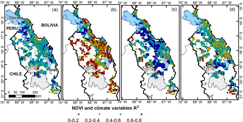
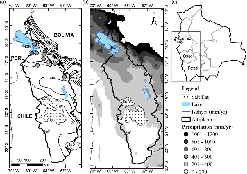
996                                            C. Canedo-Rosso et al.: Drought impact in the Bolivian Altiplano agriculture

quinoa and potato (Garcia et al., 2007). Generally speaking,        logical, agricultural, and socio-economic droughts. In more
agricultural productivity in the Bolivian Altiplano is low due      detail, a meteorological drought manifests if certain climate
to adverse weather and poor soil conditions (Garcia et al.,         variables (e.g. precipitation) remain under predefined thresh-
2003). On the other hand, low agricultural production levels        old levels over a certain time period, while hydrological
can also be associated with ENSO (Buxton et al., 2013).             drought is usually determined through reduced water levels
   The ENSO is a climate phenomenon that affects the pre-           in water bodies and groundwater. Agricultural drought oc-
cipitation variability of the Bolivian Altiplano (Thompson et       curs when insufficient soil moisture and precipitation neg-
al., 1984; Aceituno, 1988; Vuille, 1999). The ENSO is de-           atively affect crop yields, while agricultural drought may
fined as a periodical variation of the sea surface tempera-         turn into socio-economic drought if the supply or demand of
ture over the tropical Pacific Ocean, and it represents neu-        agricultural products is negatively affected (see Wilhite and
tral, warm (El Niño), and cold (La Niña) phases. The posi-          Glantz, 1985).
tive phase of ENSO is generally associated with warmer and             Using these concepts and definitions our research aims to
dryer conditions, while the negative phase is associated with       (1) classify agricultural drought severity by applying the nor-
cooling and wetter conditions (Garreaud and Aceituno, 2001;         malized difference vegetation index (NDVI; as a proxy for
Garreaud et al., 2003; Thibeault et al., 2012). Thus, droughts      crop yields), land surface temperature data, and climate data
are generally driven by the positive ENSO phase in the              (as the hazard component); (2) analyse the relationship be-
study area (Thompson et al., 1984; Garreaud and Aceituno,           tween drought and ENSO; and (3) assess drought through ex-
2001; Vicente-Serrano et al., 2015). Previous research has          amining the spatio-temporal variability of vegetation and its
addressed the influence of ENSO on agriculture in South             association with climate data (implicitly including the vul-
America and the globe (see Iizumi et al., 2014; Ramirez-            nerability component through the spatio-temporal variabil-
Rodrigues et al., 2014; Anderson et al., 2017). These studies       ity). One major constraint for drought risk management in
were calling for a better understanding of the association be-      Bolivia is the scarce and uneven distribution of weather- and
tween ENSO and agriculture to improve crop management               agricultural-production-related ground data. To circumvent
practices and food security. However, predicting the ENSO           this problem, we test satellite-based and gridded data prod-
effects is challenging, since the ENSO evolution depends not        ucts (compared to available empirically gauged data) to pro-
only on the tropic Pacific Ocean temperature, but also on           vide a full coverage (in respect to land area) for drought as-
atmospheric convection, climate variability, and teleconnec-        sessment and its spatial distribution across the region. Due
tion with other climate anomalies (Santoso et al., 2019).           to the particular importance of ENSO for drought risk man-
   The implementation of drought risk management ap-                agement, we additionally assess the impacts associated with
proaches is now seen as fundamental (see e.g. the Sustainable       ENSO on agriculture for the Bolivian Altiplano. Further-
Development Goals or the Sendai Framework for Risk Re-              more, we give indications regarding which climate variables
duction) for sustainable development in vulnerable regions,         may be most important in which regions to predict drought
including Latin American countries such as Bolivia (Verbist         losses that can further be used for hotspot selection. The pa-
et al., 2016). To lessen the long-term impacts of these ex-         per is organized as follows, Sect. 2 provides a discussion
treme events, the national government in Bolivia has taken          of the data used, Sect. 3 present the methodology applied,
several steps, e.g. to allocate budgets for emergency opera-        Sect. 4 presents the corresponding results found, and Sect. 5
tions to compensate for part of the losses incurred. Most of        ends with a conclusion and outlook for the future.
these measures are implemented ex post (i.e. after a disas-
ter event). However, based on ENSO forecasting, an El Niño
event can be predicted 1 to 7 months ahead (Tippett et al.,         2     Data Used
2012), and consequently there is an opportunity to implement
additional ex ante policies (i.e. before the event) to reduce so-   2.1    Climate data
cietal impacts of droughts, increase preparedness, and gener-
ally improve current risk management strategies.                    Our methodology is very much related to the data-scarce sit-
   We embed our research within the IPCC framework                  uation for the Bolivian Altiplano, and we therefore start with
(IPCC, 2012) and conceptually define disaster risk as a func-       an introduction of the available datasets that were used for
tion of the hazard, exposure, and vulnerability. Here, drought      our purpose. In regards to the climate dimension, the Al-
risk was defined as the likelihood of severe alterations in the     tiplano has a pronounced southwest–northeast precipitation
normal functioning due to drought hazard interacting with           gradient (200–900 mm yr−1 ) during the wet season occurring
the vulnerabilities of the exposed socio-environmental sys-         from November to March (Garreaud et al., 2003). Over 70 %
tem, leading to potential adverse effects. Furthermore, disas-      of total precipitation occurs during the summer months (from
ter risk usually comprises different types of potential losses,     December to February; see Fig. 1a) in association with the
which are sometimes very difficult to quantify (UNISDR,             South American Monsoon (see Zhou and Lau, 1998; Gar-
2009). In the case of drought, usually four different types         reaud et al., 2003). Time series of monthly precipitation at
are distinguished (UNISDR, 2009): meteorological, hydro-            12 locations as well as mean, maximum, and minimum tem-

Nat. Hazards Earth Syst. Sci., 21, 995–1010, 2021                                     https://doi.org/10.5194/nhess-21-995-2021
C. Canedo-Rosso et al.: Drought impact in the Bolivian Altiplano agriculture                                                997

perature at 8 locations from September 1981 to August 2015      tem (GLDAS) by the Noah Land Surface Model L4 monthly
were available from the National Service of Meteorology and     version 2.0 (Beaudoing and Rodell, 2019). The dataset was
Hydrology (SENAMHI) of Bolivia (see Appendix Table A1).         available for the study period September 1981 to August
These datasets had less than 10 % of missing data and there-    2015. The LST estimations from GLDAS were based on re-
fore served well for our analysis.                              motely sensed observations of AVHRR (Rodell et al., 2004)
   As already indicated, precipitation and temperature gauge    and include an algorithm that relies on an optimal interpo-
locations are unevenly distributed and mainly concentrated      lation routine (Ottlé and Vidal-Madjar, 1992) to assimilate
in the northern Bolivian Altiplano. To improve the spatial      the LST onto a 0.25◦ by 0.25◦ grid. This data record was
coverage of climate-related data, monthly quasi-rainfall time   selected due to its temporal resolution; however, it is impor-
series from satellite data the Climate Hazards Group In-        tant to mention that a higher spatial resolution could improve
fraRed Precipitation with Station data (CHIRPS) were in-        the accuracy of agricultural analyses and further reduce the
cluded in our study. CHIRPS represents a 0.05◦ spatial res-     uncertainties of the data noise originating from land hetero-
olution satellite imagery and a quasi-global rainfall dataset   geneity.
from 1981 to the near present (Funk et al., 2015). The ad-         Finally, the study was conducted for the agricultural land
vantage of using CHIRPS is the high spatial resolution of       in the Bolivian Altiplano (∼ 200 000 km2 ). The agricultural
data, obtained with resampling of TMPA 3B42 (with a 0.25◦       land was spatially identified based on the land use map de-
grid cell). The spatial resolution represents a better option   veloped by the Autonomous Authority of the Lake Titicaca
for agricultural studies as well and therefore is most appro-   (for the northern Altiplano) in 1995 at a scale of 1 : 250 000
priate for our approach (CHIRPS is described in detail at       (UNEP, 1996) and the Ministry of Development Planning
https://www.chc.ucsb.edu/data/chirps, last access: 22 Febru-    in 2002 using Landsat imagery and ground information at
ary 2021).                                                      a scale 1 : 1 000 000 (http://geo.gob.bo/portal/, last access:
   Additionally, a gridded dataset of monthly mean air tem-     15 May 2019, for the southern Altiplano).
perature was obtained from the Physical Sciences Divi-
sion (PSD) of the US National Oceanic and Atmospheric
Administration (NOAA, https://www.esrl.noaa.gov/psd/, last      3     Methodology
access: 1 May 2020) defined by Willmott and Matsuura,
using a spatial interpolation of composite stations records     The analysis of drought impact on agriculture for the Boli-
from the Global Historical Climatology Network (GHCN            vian Altiplano and its relationship with the ENSO is based
version 2) and Legates and Willmott (Legates and Willmott,      on the following three steps. Firstly, an evaluation of satel-
1990a; Legates and Willmott, 1990b). The gridded air tem-       lite precipitation and gridded air temperature against gauged
perature dataset has a resolution of 0.5◦ by 0.5◦ and was       datasets was performed to investigate the accuracy of these
available during the study period from September 1981 to        estimates compared to empirical on-the-ground data. Sec-
August 2015. This dataset incorporates station-height infor-    ondly, the severity of drought was classified using vegetation
mation through an average air temperature lapse rate (Will-     and land surface temperature data, and using this information
mott and Matsuura, 1995). Here, a digital elevation model       drought events were associated with the ENSO variability.
was used for the interpolation to adjust air temperatures in    Finally, a stepwise regression approach was used to study
relation to sea level.                                          the variability of vegetation and its relationship with corre-
                                                                sponding climate variables. The overall aim of our study is to
2.2   Land surface data: vegetation and temperature             investigate drought effects on agriculture through the analy-
                                                                sis of land surface and climate variations and their relation to
Apart from climate datasets, NDVI was assembled from            the ENSO anomalies.
the Advanced Very High Resolution Radiometer (AVHRR)
sensors by the Global Inventory Monitoring and Modelling        3.1    Evaluation of climate data
System (GIMMS) at semi-monthly (15 d) time steps with
a spatial resolution of 0.08◦ . NDVI 3g.v1 (third generation    The performance of the satellite-based data (compared to
GIMMS NDVI from AVHRR sensors) was available from               empirical ground data; see Fig. 2) in accurately estimating
September 1981 to August 2015. The NDVI is an index that        the amount of rainfall (for example rain detection capabil-
presents a range of values from 0 to 1, and bare soil values    ity purposes) was based on statistical measures for monthly
are closer to 0, while dense vegetation is close to 1 (Hol-     pairwise time series, including categorical analyses, and fol-
ben, 1986). NDVI 3g.v1 GIMMS provides information to            lows methodologies suggested and applied in previous stud-
differentiate valid values from possible errors due to snow,    ies in this region, which were selected for comparison rea-
cloud, and interpolation. These errors were removed from the    sons (Blacutt et al., 2015; Satgé et al., 2016). The mean er-
dataset and replaced with the nearest-neighbour value.          ror (ME), bias, and mean absolute error (MAE) were calcu-
   Additionally, the monthly land surface temperature (LST)     lated based on Wilks (2006). These measures evaluate the
was obtained from the Global Land Data Assimilation Sys-        prediction accuracy of the satellite data compared to gauged

https://doi.org/10.5194/nhess-21-995-2021                                Nat. Hazards Earth Syst. Sci., 21, 995–1010, 2021
998 C. Canedo-Rosso et al.: Drought impact in the Bolivian Altiplano agriculture Figure 1. (a) Gauged mean monthly total precipitation and average maximum and minimum temperature from September 1981 to Au- gust 2015. (b) Mean monthly NDVI at the same spatial locations. Lower and upper box boundaries show the 25th (Q1 ) and 75th (Q3 ) percentiles, respectively; the line inside the box is the median; the lower and upper error lines indicate 1.5 times the interquartile range (Q3 –Q1 ) from the top or bottom of the box; white circles represent data falling outside 1.5 times the interquartile rage. data. The ME and bias show the degree of over- or underes- gauged data was calculated using the arithmetic mean be- timation (Duan et al., 2015). In contrast, as with measuring tween the maximum and minimum temperature. The regres- the absolute deviation, MAE shows only non-negative val- sion performance was evaluated using the monthly pairwise ues. The ME, bias, and MAE perfect match corresponds to time series to define the Spearman rank correlation, relative zero between gauge observation and satellite-based estimate. ME, bias, and MAE. For air temperature, the MAE was de- Furthermore, and similar to Blacutt et al. (2015) and Satgé fined using absolute values. et al. (2016), the Spearman rank correlation was computed to estimate the goodness of fit to observations. To evaluate 3.2 Drought associated with ENSO results, and in accordance with similar studies, correlation coefficients larger or equal to 0.7 were considered reliable Healthy vegetation usually shows enlarged near infrared and (Condom et al., 2011; Satgé et al., 2016). The ME, bias, and reduced visible bands and emits less absorbed thermal in- MAE were calculated according to Eqs. (1), (2), and (3) in frared radiation, resulting in lower surface temperature (Ko- Table 1, respectively. gan and Guo, 2017). Therefore, vegetation indices and land Two statistical indicators based on contingency tables surface temperature (LST) are widely used for water and en- were computed for the categorical statistics, namely proba- ergy balance approaches (see Moran et al., 1994; Corbari et bility of detection (POD) and false alarm ratio (FAR). The al., 2010; Sánchez et al., 2012; Helman et al., 2015). Pre- POD indicates what fraction of the observed events was cor- vious findings indicate a negative (positive) relationship be- rectly estimated, and FAR indicates the fraction of the pre- tween LST and NDVI caused by limited moisture (energy- dicted events that did not occur (Bartholmes et al., 2009; temperature) availability for vegetation growth (Karnieli et Ochoa et al., 2014; Satgé et al., 2016). The POD and FAR al., 2010). Drought spells typically present low NDVI and range from 0 to1, where 1 is a perfect score for POD, and 0 high LST due to vegetation deterioration and higher con- is a perfect score for FAR. These measures were used to eval- tribution of the soil signal (Kogan, 2000). Here, we study uate the satellite precipitation estimations. Here, the rainfall the relationship between LST and NDVI using the vegeta- amounts are considered as binary values, i.e. rain occurrence tion health index (VHI, Eq. 8) developed by Kogan (1995) or absence. Based on this approach, three counting variables that combines the vegetation condition index (VCI, Eq. 6) were taken into account: the number of events when the satel- and temperature condition index (TCI, Eq. 7). VCI compares lite rain estimation and the rain gauge report a rain event (hit the current NDVI with the range of NDVI observations dur- or H), when only the satellite reports a rain event but no rain ing the study period that allows us to seek the variability of on the ground is observed (false alarm or F), and when only the signal, showing an increased VCI when NDVI increases. the rain gauge reports a rain event but not the satellite and (Kogan, 1995; Kogan, 2000; Kogan and Guo, 2017). In con- therefore is a miss (M). The POD and FAR were calculated trast, the TCI formulates a reverse ratio compared to the VCI, according to Eqs. (4) and (5) in Table 1, respectively. decreasing when LST increases, assuming that higher land Besides the precipitation data, the gridded air temperature surface temperatures suggest a decreasing soil moisture caus- data were evaluated using ground data. The gridded air tem- ing stress of the vegetation canopy. perature was correlated with the mean gauged temperature The VCI, TCI, and VHI was defined for each month dur- at the same spatial location. The mean temperature of the ing the growing season (from September to April). We as- Nat. Hazards Earth Syst. Sci., 21, 995–1010, 2021 https://doi.org/10.5194/nhess-21-995-2021
C. Canedo-Rosso et al.: Drought impact in the Bolivian Altiplano agriculture                                                       999

Table 1. Accuracy measures for the performance evaluation of climate estimated variables. Here, N is the number of samples, Si is the
climate estimation for month i, and Gi is the gauged dataset for the same month. H is a hit, F is a false alarm, and M is a miss.

                       Statistical indicator      Abbreviation    Units                    Equation
                                                                  mm, ◦ C
                                                                             P
                       Mean error                 ME                         P (Si − Gi ) / P
                                                                                            N                  (1)
                       Bias                       Bias            %          P (Si − Gi ) / Gi × 100           (2)
                       Mean absolute error        MAE             %             |(Si − Gi ) / Gi | / N × 100   (3)
                       Probability of detection   POD             –          H / (H + M)                       (4)
                       False alarm ratio          FAR             –          F / (H + F )                      (5)

Figure 2. Mean of total annual precipitation from September 1981 to August 2015 for (a) gauged precipitation data (circles) and isohyets
(solid line), (b) the CHIRPS satellite rainfall product, and (c) major political divisions of Bolivia.

sumed the occurrence of a drought event when the indices              For this study, a neutral or weak phase was defined as a
were lower than 40 %. The classification of drought was es-           threshold between the −0.9 and +0.9 ◦ C anomaly.
tablished based on the severity of the event in which five
classes were defined: extreme (≤ 10), severe, (≤ 20), mod-            3.3   Regression of vegetation and climate variables
erate (≤ 30), mild (≤ 40), and no (> 40) drought (Bhuiyan
and Kogan, 2010).                                                     A stepwise regression approach was used to quantify the de-
   The drought events were further classified based on the oc-        pendency between vegetation and climate variables (satellite-
currence of El Niño and La Niña events (Table 3). The classi-         based precipitation and gridded air temperature; Eq. 10) to be
fication ENSO was obtained from Null (2018). El Niño and              used for the hotspot selection process. In more detail, the re-
La Niña events were identified from five consecutive over-            sults presented here are a combination of forward and back-
lapping 3-month mean sea surface temperatures for the Niño            ward selection techniques to increase the robustness of the
3.4 region (in the tropical Pacific Ocean). A moderate El             results (in terms of explanatory power, i.e. variability ex-
Niño (La Niña) was defined as five consecutive overlapping            plained, as well as variable selection, i.e. same variable se-
3-month periods at or above the +1.0 to +1.4 ◦ C anomaly              lected across a range of possible models). The independent
(−1.0 to −1.4 ◦ C), a strong El Niño (La Niña) event for a            variable considered was NDVI, and the dependent variables
threshold between the +1.5 and +1.9 ◦ C anomaly (−1.5 to              were selected to include precipitation and air temperature
−1.9 ◦ C anomaly), and a very strong El Niño event for a              (for the same spatial location across the study region). We as-
threshold equal to or greater than the +2 ◦ C anomaly (https:         sumed that NDVI represents the crop phenological stages of
//ggweather.com/enso/oni.htm, last access: 15 May 2020).              the growing season that is from September to April (Fig. 1).
                                                                      Precipitation was selected as a predictor due to its relevance

https://doi.org/10.5194/nhess-21-995-2021                                      Nat. Hazards Earth Syst. Sci., 21, 995–1010, 2021
1000 C. Canedo-Rosso et al.: Drought impact in the Bolivian Altiplano agriculture
Table 2. Drought classification indices.
Drought index Abbreviation Equation
Vegetation condition index VCI (NDVIi − NDVImin ) / (NDVImax − NDVImin ) (6)
Temperature condition index TCI (LSTmax − LSTi ) / (LSTmax − LSTmin ) (7)
Vegetation health index VHI 0.5 VCI + 0.5 TCI (8)
Here, NDVIi (LSTi ) is the monthly NDVI (LST) and NDVImax and NDVImin (LSTmax and LSTmin ) are its multi-year absolute
maximum and minimum (1981–2015), respectively. We took a mean of VCI and TCI assuming that they equally contribute to the VHI.
Table 3. El Niño and La Niña phases (from Null, 2018).
El Niño La Niña
Moderate Strong Very strong Moderate Strong
1986–1987 1987–1988 1982–1983 1995–1996 1988–1989
1994–1995 1991–1992 1997–1998 2011–2012 1998–1999
2002–2003 2015–2016 1999–2000
2009–2010 2007-2008
2010–2011
for water availability for vegetation growth. Precipitation is 1995). The results were compared with results from the lit-
the main source of water in the Altiplano because only 9 % erature regarding phenology and weather-related characteris-
of the Bolivian cropped surface area is irrigated (INE, 2015). tics of crops.
Air temperature is a relevant variable due to photosynthetic It should be noted that the precipitation in the Altiplano
and respiration processes (Karnieli et al., 2010). Firstly, the shows a marked rainy season from November to March. The
NDVI was related to CHIRPS rainfall datasets. Secondly, peak of precipitation is in December and January (Fig. 1a).
air temperature was included in the analysis. Here, only the Additionally, NDVI displays a peak in March and April
NDVI grids for agricultural land were selected. Since, agri- (Fig. 1b). The lag between the precipitation and NDVI is
cultural production data are scarce in the region, we suggest reasonable since vegetation requires time to grow (e.g. Shin-
that crop yield data can be improved using the NDVI. Be- oda, 1995; Cui and Shi, 2010; Chuai et al., 2013). Consider-
sides improving the crop yield resolution, the NDVI also al- ing this lag time, the 3-month time series of NDVI was re-
lows us to analyse the variability of vegetation at a monthly gressed with the 3-month time series of the climate variables
timescale. This makes it possible to analyse the phenology (satellite-based data product of precipitation and gridded data
of the studied crops through to the growth phases. NDVI es- of air temperature) during the growing period for the agricul-
timates the vegetation vigour (Ji and Peters, 2003) and crop tural land. First, the NDVI and the climate variables were
phenology (Beck et al., 2006). The final regression model for related considering the overlapping 3-month time series, and
each spatial unit was defined as afterwards a relation was developed considering a lag from
1 to 4 months between NDVI and climate variables, result-
NDVI = β0 + β1 precipitation + β2 air temperature. (1) ing in 22 regressions per NDVI grid. The regressions were
developed for each NDVI grid separately, associated with
For the forward selection, the variables were entered into the nearest precipitation and air temperature dataset. Prior
the model one at a time in an order determined by the strength to the stepwise regression analysis, the 3-month time series
of their correlation with the criterion variable (only including of NDVI, satellite precipitation, and gridded air temperature
variables if they present a confidence level of 95 %). The ef- data were standardized.
fect of adding each variable was assessed during its entering
stage, and variables that did not significantly add to the fit of
the model were excluded (Kutner et al., 2004). For backward 4 Results
selection, all predictor variables were entered into the model
first. The weakest predictor variable was then removed and Validation of the satellite rain data using empirical precip-
the regression fit re-calculated. If this significantly weakened itation data from the weather stations was done for the 12
the model, then the predictor variable was re-entered; other- locations where gauge precipitation data were available (see
wise it was deleted. This procedure was repeated until only Fig. 2 and Table A1). The qualitative methods discussed in
useful predictor variables (in a statistical sense, e.g. signifi- Sect. 3.1 for the CHIRPS rainfall estimates show differences
cant as well as model fit) remained in the model (Rencher, between summer (from December to March) and winter sea-
Nat. Hazards Earth Syst. Sci., 21, 995–1010, 2021 https://doi.org/10.5194/nhess-21-995-2021C. Canedo-Rosso et al.: Drought impact in the Bolivian Altiplano agriculture 1001 son (from June to August). CHIRPS data show better ac- due to the estimation uncertainties, mainly during winter sea- curacy during summer. The precipitation during the austral son. summer is highly relevant because it concentrates the 70 % As discussed above, the VCI, TCI, and VHI were calcu- of the annual rainfall (Garreaud et al., 2003), and it occurs lated during the growing season. The sowing period depends during the growing season. During May, CHIRPS data show on the initial soil moisture content; therefore the beginning of lower accuracy compared to the other months. The precipi- the growing season oscillates from September to November tation from May to August is almost null in the study area (Garcia et al., 2015). For this reason, the drought severity was (Fig. 1), and it will be further described as the dry season. classified considering the mean of VCI, TCI, and VHI for the This season presents stable atmospheric conditions with few agricultural land during November–April. Figure A1 shows precipitation events (Garreaud et al., 2003). mean monthly VCI from November 1981 to April 2015. The Interestingly, the Spearman rank correlation between major drought events (severe or extreme) are visible in 1982– monthly gauged precipitation and satellite rain product 1983, 1983–1984, and 2009–2010, followed by moderate datasets was significant (p value < 0.05) for all loca- drought events during 1987–1988 and 1993–1994, as well tions. The correlation coefficients (r) vary from 0.5 to 0.8 as several mild events. Figure A2 shows the mean monthly (mean = 0.7). The ME and bias disclose an underestima- TCI, where the major drought events (severe or extreme) oc- tion of precipitation estimation during October, November, curred in 1982–1983, 1987–1988, 1997–1998, 2004–2005, and April and an overestimation during the summer season and 2009–2010, followed by moderate drought events during (mean = 5 mm and 7 %, respectively) with a peak in Febru- 1981–1982, 1983–1984, 1994–1995, 2006–2007, and 2008– ary. For the MAE coefficient, CHIRPS estimations are more 2009, and several mild events as well. Finally, Fig. A3 shows accurate during the rainy season (mean = 31 %). In contrast, the VHI results, in which the major drought events occurred CHIRPS data indicate poor accuracy during the dry sea- during 1982–1983, 2004–2005, and 2009–2010. son (mean MAE = 92 %). From June to August, CHIRPS In a next step we related drought indices with the ENSO data present an underestimation of the gauged precipitation phases (Table 4). Extreme and severe droughts were gener- (mean bias = −39 %). Summarizing these observations, we ally found during the El Niño phase. The extreme drought of conclude that the CHIRPS rainfall dataset is more accurate 1982–1983 coincided with a very strong El Niño phase. For during the rainy season, and it represents an adequate alter- this event, the largest economic losses caused by droughts native in case of lack of gauged data or in case of poor data during the study period are reported (Table 5), followed by quality. However, it should be noted that such data still must the very strong El Niño phase of 1997–1998, which re- be used with caution considering the uncertainties due to the ported the second largest economic losses. Besides these two under- or overestimation of precipitation along the heteroge- main drought events, the strong El Niño during 1987–1988 neous topography of the Altiplano (see Paredes-Trejo et al., coincided with an extreme/moderate drought (TCI ≤ 10 %, 2016; Paredes-Trejo et al., 2017; Rivera et al., 2018). VCI ≤ 30 %) classification. During this period, large eco- Moving from rainfall to temperature, the inter-annual tem- nomic losses were reported as well (Table 5). In contrast, perature at the eight locations varied considerably between the strong El Niño during 1991–1992 showed low severity summer (from December to March) and winter (from June to (mild drought VCI ≤ 40 %), and no economic losses were August), including a larger variance for the minimum tem- reported. This indicates that despite the fact that the El perature (Fig. 1a). The mean monthly air temperature from Niño phenomenon is generally associated with drought in gridded data was compared with mean temperature of gauged the Altiplano, there are several other mechanisms that drive a data. The gridded air temperature underestimated the mean drought occurrence and determine its severity. For instance, gauged temperature, and this error could be due to the hetero- dry (wet) and warm (cool) conditions during El Niño (La geneous topography and high elevation. The Spearman cor- Niña) phases are generally shown in the Altiplano (Garreaud relation at the eight stations displayed coefficients from 0.1 et al., 2003). However, an anomalous location and inten- to 0.7. From November to April, the gridded air temperature sity of zonal wind anomalies could cause disturbances of the data show significant correlations (p value < 0.05). Large warming and cooling air patterns causing rainfall anomalies correlations are shown during summer season (mean = 0.7), in the region (Garreaud and Aceituno, 2001). This is the case while the other months show rather weak correlations. ME of the dry La Niña during 1988–1989 that showed a mild and bias show a slight underestimation from October to April drought classification (TCI ≤ 40 %). (mean = −0.5 ◦ C and −4 % respectively) and an overesti- One severe (1983–1984) and one extreme (2004–2005) mation from May to August (mean = 0.3 % and 12 % re- event occurred during a neutral/weak ENSO. The severe spectively). Finally, MAE is about 1.2 ◦ C from September drought (VCI ≤ 20 %) occurred during a neutral phase of to April, and higher values develop during winter season 1983–1984. This coincides with the findings of Vicente- (mean = 1.6 ◦ C). In conclusion, the gridded air temperature Serrano et al. (2015) that analysed the standardized pre- data product performs better from November to April. Sim- cipitation/evaporation index in Bolivia, which is an alter- ilar to the precipitation data, the application of gridded air native technique to characterize a meteorological drought. temperature data must take into account the potential errors The extreme drought (TCI ≤ 10 %) of 2004–2005 occurred https://doi.org/10.5194/nhess-21-995-2021 Nat. Hazards Earth Syst. Sci., 21, 995–1010, 2021
1002                                            C. Canedo-Rosso et al.: Drought impact in the Bolivian Altiplano agriculture

Figure 3. Monthly accuracy measures of CHIRPS rainfall data product. Mean monthly values are represented by black circles, and bars
represent the standard error of the mean.

Figure 4. Same as Fig. 3 but for accuracy measures of the gridded air temperature data product.

in November and December. From January to April of 2004–                   Regarding the relationship between vegetation and cli-
2005 the VCI and VHI were above 40 %, and there were no                 mate variables, we note that the precipitation season occurs
claims of drought losses in the Altiplano for this particular           mainly during the austral summer months (from December
year (Table 5). Besides these two events, moderate and mild             to March), and the vegetation development shows a lag with
droughts also occurred during non-El Niño phases.                       a maximum development around March and April (Fig. 1).
   Table 5 shows that five drought events were reported dur-            The NDVI (Fig. 1b) shows a similar growing pattern to the
ing a neutral ENSO phase. In 2012–2013, the largest im-                 crop phenology in the region, which starts in September and
pact occurred, affecting about 80 000 people in the Altiplano           ends in April. Maximum and minimum temperature varies
(Desinventar Sendai, 2020). Despite the fact that the mean of           during the year. Higher temperature during the austral sum-
the drought indices indicates no drought during this period             mer leads to higher evapotranspiration and a decrease in wa-
(VCI, TCI, and VHI > 40 %), some spatial locations in the               ter retained in the root zone. With this presumption, stepwise
study region indicated the occurrence of a drought event in             linear regression models were tested using 3-month time se-
November and December (21 % and 29 % of the total stud-                 ries of NDVI as the dependent variable and 3-month time se-
ied grids showed mild and moderate droughts for the TCI and             ries of satellite-based data product of precipitation and grid-
VCI respectively).                                                      ded air temperature as independent variables (Eq. 10). The

Nat. Hazards Earth Syst. Sci., 21, 995–1010, 2021                                        https://doi.org/10.5194/nhess-21-995-2021
C. Canedo-Rosso et al.: Drought impact in the Bolivian Altiplano agriculture                                                        1003

Table 4. Drought index classification during ENSO phases.

  ENSO            Drought      VCI                                  TCI                              VHI
  El Niño         Extreme                                           1982–1983, 1987–1988, 1997–
                                                                    1998
                  Severe       1982–1983, 2009–2010                 2009–2010                        1982–1983, 2009–2010
                  Moderate     1987–1988                            1994–1995
                  Mild         1986–1987, 1991–1992                 1986–1987                        1994–1995, 1997–1998
  La Niña         Mild         1995–1996, 2007–2008, 2010–          1988–1989
                               2011
  Neutral/weak    Extreme                                           2004–2005
                  Severe       1983–1984
                  Moderate     1993–1994                            1981–1982, 1983–1984, 2006–      2004–2005
                                                                    2007, 2008–2009
                  Mild         1981–1982, 1996–1997, 2003–          1984–1985 1990–1991, 1993–       1981–1982, 1983–1984, 1990–
                               2004, 2008–2009                      1994, 2014–2015                  1991, 1993–1994, 2005–2006,
                                                                                                     2008–2009

Table 5. Drought impact in Bolivia (from EM-DAT, 2020, BID,               that the NDVI depends largely on the studied climate vari-
2016, and CAF, 2000).                                                     ables. This may be due to the crop’s sensitivity for water
                                                                          stress during specific stages of the growing season. For in-
 Year         ENSO phase     Affected people   Total damage               stance the most sensitive stages of the quinoa crop are the
                                               (thousands of USD)
                                                                          emergence, flowering, and grain development (see Geerts et
 1982–1983    El Niño        3 083 049         917 200                    al., 2008; Geerts et al., 2009), as well as the near absence of
 1987–1988    El Niño                          48 400                     irrigation practices in most of these regions.
 1989–1990    Neutral        283 160
 1997–1998    El Niño                          279 310
                                                                             In more detail, the stepwise regression results for the over-
 1993–1994    Neutral        50 000                                       lapping 3-month time series of NDVI and climate variables
 1999–2000    La Niña        20 000                                       for SON (September, October, and November) show statis-
 2003–2004    Neutral        55 000                                       tically significant coefficients for precipitation and air tem-
 2007–2008    La Niña        27 500
                                                                          perature at 45 % and 98 % of the agricultural area in the Bo-
 2009–2010    El Niño        62 500            100 000
 2012–2013    Neutral        340 355                                      livian Altiplano with a median of 0.2 and 0.7, respectively
 2013–2014    Neutral        51 180                                       (Fig. 5a). This indicates that the NDVI increases with more
                                                                          rain and higher air temperature. Interestingly, the significant
                                                                          regression coefficients of NDVI for OND (October, Novem-
                                                                          ber, and December) associated with precipitation and air tem-
stepwise regression was defined considering the overlapped                perature for SON cover 64 % and 91 % of the agricultural
3-month time series and the 3-month time series with a lag                area and have a positive median of 0.3 and 0.4, respectively
from 1 to 4 months at the same spatial location over the agri-            (Fig. 5b). A time lag of 1 month shows larger spatial cover-
cultural land.                                                            age of the response of vegetation to precipitation anomalies.
   The results of the stepwise regression show a larger coeffi-           Here, the largest coefficient of determination are shown in
cient of determination (R 2 ) in the northern and central Boli-           areas surrounding the Lake Titicaca. Moreover, the response
vian Altiplano, starting from the southern Lake Titicaca and              of the NDVI for MAM (March, April, and May) to the stud-
moving southwards to Lake Poopó, and close to the rivers’                 ied climate anomalies for FMA (February, March, and April)
paths. Lower R 2 values are shown along the southwestern                  covers 95 % and 96 % of the agricultural land for precipita-
Bolivian Altiplano that could be explained through the large              tion and air temperature, respectively (Fig. 5c). This mostly
variance of the NDVI, which may depend to on other factors                shows coefficients of determination ranging from 0.4 to 0.8,
besides precipitation and temperature, including crop man-                and positive regression coefficients for precipitation and air
agement. Figure 5 shows the R 2 of the best fit regression in             temperature have a median of 0.5 and 0.4, respectively. The
the Bolivian Altiplano for the 3-month period of NDVI and                 hours of sun required for crop development could be an ex-
the climate variables (precipitation and temperature) during              planation for the time lag between vegetation and the climate
the beginning and end of the growing season. It can be seen

https://doi.org/10.5194/nhess-21-995-2021                                         Nat. Hazards Earth Syst. Sci., 21, 995–1010, 2021
1004 C. Canedo-Rosso et al.: Drought impact in the Bolivian Altiplano agriculture
Figure 5. Coefficient of determination (R 2 ) of NDVI for the 3-month time series for (a) SON, (b) OND, (c) MAM, and (d) MAM and the
climate variables (satellite precipitation and gridded air temperature products) for SON, SON, FMA, and MAM respectively. The significant
regression coefficients for precipitation (air temperature) cover (a) 45 % (98 %), (b) 64 % (91 %), (c) 95 % (96 %), and (d) 23 % (98 %) of
the total studied grids that represent the agricultural land.
variables. In addition, the lag differences between vegetation air temperature. However, in prolonged dry periods, high air
and precipitation can be partly explained by the topography, temperature could increase the evapotranspiration rates and
land cover, groundwater, and soil properties (Quiroz et al., consequently decrease the soil moisture (Huang et al., 2019).
2011; Yarleque et al., 2016). Finally, the regression for NDVI This scenario could impact negatively the vegetation, as this
and climate variables for the overlapped 3-month time series is the case of the drought events of 1982–1983 and 1997–
of MAM shows significant coefficients at 23 % and 98 % of 1998, where large production losses were reported (Santos,
the agricultural land, with a median of 0.4 and 0.6 for pre- 2006).
cipitation and air temperature, respectively (Fig. 5d). Hence,
the vegetation response to precipitation is limited for the last
overlapped 3-month time series of the growing season. How- 5 Discussion and conclusion
ever, it should be noted that air temperature remains an im-
portant variable. We employed satellite-based and gridded dataset products
To summarize, while acknowledging some important lim- and tested the dataset’s empirical accuracy as well as per-
itations, we found that the CHIRPS dataset is adequate to formance to similar (but with coarser resolution) datasets
be used for drought risk assessment in case of severe data available for the Bolivian Altiplano region. Spatio-temporal
scarcity for the Bolivian Altiplano. Furthermore, we found patterns of satellite precipitation and gridded air tempera-
that the vegetation variance can be significantly explained by ture anomalies were explored based on monthly time series
precipitation and air temperature. More specifically, we point during the period September 1981 to August 2015. Drought
out the relevance of precipitation as the main water source severity was evaluated based on a drought classification
for vegetation development and air temperature as a driver scheme using NDVI and LST; this classification was related
of photosynthetic processes. Precipitation is particularly im- with the ENSO anomalies. Finally, association between the
portant at the early and late phenological stages, in which spatial distribution of NDVI with precipitation and air tem-
crops are more sensitive to water shortage. This is the case perature was examined. Using these datasets, it was shown
for the main crops in the region, i.e. quinoa and potato. For that drought severity (measured through various drought in-
the quinoa crop, the most sensitive phases to water stress are dices) increases substantially during El Niño years, and as
the emergence, flowering, and grain development (see Geerts a consequence the socio-economic drought risk of farmers
et al., 2008; Geerts et al., 2009). The most sensitive phases of will likely increase during such periods. ENSO forecasts as
the potato crop to water stress is the tuber initiation and bulk- well as drought severity (through drought indices) can help to
ing (van Loon, 1981; Alva et al., 2012). On the other hand, determine possible hotspots of crop deficits during the grow-
air temperature is relevant for vegetation productivity, and ing season. The empirical relationships of land surface and
overall we found a positive relation between vegetation and climate data on the local scale of our approach can support
a proactive approach to disaster risk management against
Nat. Hazards Earth Syst. Sci., 21, 995–1010, 2021 https://doi.org/10.5194/nhess-21-995-2021C. Canedo-Rosso et al.: Drought impact in the Bolivian Altiplano agriculture 1005 droughts, through an evaluation of the evolution of climate anomalies (in this case the ENSO) and their potential adverse effects in the region. As it was shown here, the ENSO-warm- phase-related characteristics are especially important in the context of extreme drought events and could therefore be in- corporated within early warning systems as standard prac- tice. Despite these challenges for the development of drought early warning systems (see FAO, 2016, 2017), applications have been successful in the past (e.g. Global Information and Early Warning System (GIEWS) of FAO and Famine Early Warning System (FEWS) of USAID). Monitoring and pre- dicting ENSO can therefore significantly contribute to reduce the risk of disasters. This study is a first attempt to provide an assessment of drought impact on agriculture in relation to the ENSO phenomenon for the Bolivian Altiplano. We fo- cused on where vegetation is more affected by droughts over agricultural land and how this can be clarified using satellite imagery. It is important to note that the variance of drought indices (as well as NDVI) to a large extent is explained by precipitation and air temperature anomalies in the studied region. The agriculture in this semi-arid region is ecologi- cally fragile, and the main water source is precipitation, and thus crop production is considerably affected by precipitation anomalies. However, while an overall response of vegetation variance to precipitation and air temperature is evident, it is important to consider other variables, such as evapotranspira- tion and soil moisture to improve risk-based models. Another important issue is the time lag of the response of vegetation to precipitation and air temperature anomalies, which shows a hysteresis of 1–2 months. These findings provide informa- tion for future drought risk management and early warning system applications. In addition, with such information agri- cultural models can be set up along with risk management plans with improved accuracy. https://doi.org/10.5194/nhess-21-995-2021 Nat. Hazards Earth Syst. Sci., 21, 995–1010, 2021
1006                                                  C. Canedo-Rosso et al.: Drought impact in the Bolivian Altiplano agriculture

Appendix A

Table A1. Spatial location of the studied weather stations where
gauged precipitation data are available; the stations that also present
temperature maximum and minimum data are indicated by T on the
temperature column.

 No.   Station name         Latitude   Longitude   Altitude   Temperature
 1     Ayo Ayo               −17.1        −68.0       3888
 2     Calacoto              −17.3        −68.6       3830    T
 3     Collana               −16.9        −68.3       3911    T
 4     El Alto Aeropuerto    −16.5        −68.2       4034    T             Figure A2. Same as Fig. A1 but for the TCI.
 5     El Belen              −16.0        −68.7       3833    T
 6     Oruro Aeropuerto      −18.0        −67.1       3701    T
 7     Patacamaya            −17.2        −67.9       3793
 8     Salla                 −17.2        −67.6       3500
 9     San Juan Huancollo    −16.6        −68.9       3829
 10    Santiago de Huata     −16.1        −68.8       3845    T
 11    Tiahuanacu            −16.6        −68.7       3863    T
 12    Viacha                −16.7        −68.3       3850    T

                                                                            Figure A3. Same as Fig. A1 but for the VHI.

Figure A1. Monthly mean VCI (%) from November 1981 to
April 2015. Solid line indicates the minimum monthly value along
the study period. Values below 40% (dashed line) represent a
drought event.

Nat. Hazards Earth Syst. Sci., 21, 995–1010, 2021                                            https://doi.org/10.5194/nhess-21-995-2021
C. Canedo-Rosso et al.: Drought impact in the Bolivian Altiplano agriculture 1007
Code availability. For analysis we have used the MATLAB pro- Anderson, W., Seager, R., Baethgen, W., and Cane, M.: Life
gramming language. A script file is available in the Supplement. cycles of agriculturally relevant ENSO teleconnections in
North and South America, Int. J. Climatol., 37, 3297–3318,
https://doi.org/10.1002/joc.4916, 2017.
Data availability. The data used in the study are open and down- Bartholmes, J. C., Thielen, J., Ramos, M. H., and Gentilini,
loadable at the websites: http://senamhi.gob.bo/index.php/sismet S.: The european flood alert system EFAS – Part 2: Statis-
(SENAMHI 2019), https://data.chc.ucsb.edu/products/CHIRPS-2. tical skill assessment of probabilistic and deterministic op-
0/global_monthly/netcdf/ (Funk, 2015), https://psl.noaa.gov/data/ erational forecasts, Hydrol. Earth Syst. Sci., 13, 141–153,
gridded/data.UDel_AirT_Precip.html (Willmott and Matsuura, https://doi.org/10.5194/hess-13-141-2009, 2009.
2001), https://doi.org/10.5067/9SQ1B3ZXP2C5 (Beaudoing and Beaudoing, H. and Rodell, M.: NASA/GSFC/HSL: GLDAS
Rodell, 2019), https://climatedataguide.ucar.edu/climate-data/ndvi- Noah Land Surface Model L4 monthly 0.25 × 0.25 de-
normalized-difference-vegetation-index-3rd-generation-nasagfsc- gree V2.0, Greenbelt, Maryland, USA, Goddard Earth Sci-
gimms (Pinzon and Tucker, 2018). ences Data and Information Services Center (GES DISC),
https://doi.org/10.5067/9SQ1B3ZXP2C5, 2019.
Beck, P. S. A., Atzberger, C., Høgda, K. A., Johansen,
Supplement. The supplement related to this article is available on- B., and Skidmore, A. K.: Improved monitoring of vegeta-
line at: https://doi.org/10.5194/nhess-21-995-2021-supplement. tion dynamics at very high latitudes: A new method us-
ing MODIS NDVI, Remote Sens. Environ., 100, 321–334,
https://doi.org/10.1016/j.rse.2005.10.021, 2006.
Bhuiyan, C. and Kogan, F. N.: Monsoon variation and veg-
Author contributions. CCR conceived the study, collected the data,
etative drought patterns in the Luni Basin in the rain-
performed the analysis, interpreted the results, and wrote the article.
shadow zone, Int. J. Remote Sens., 31, 3223–3242,
SHS, GP, BC, and RB contributed to the writing and the interpreta-
https://doi.org/10.1080/01431160903159332, 2010.
tion of the results.
BID: Analisis ambiental y social, in: Programa de Saneamiento del
Lago Titicaca, Banco Interamericano de Desarrollo (BID), La
Paz, Bolivia, 2016.
Competing interests. The authors declare that they have no conflict Blacutt, L. A., Herdies, D. L., de Gonçalves, L. G. G.,
of interest. Vila, D. A., and Andrade, M.: Precipitation compari-
son for the CFSR, MERRA, TRMM3B42 and Combined
Scheme datasets in Bolivia, Atmos. Res., 163, 117–131,
Acknowledgements. The authors want to thank the reviewers for https://doi.org/10.1016/j.atmosres.2015.02.002, 2015.
their thoughtful comments and efforts towards improving our pa- Buxton, N., Escobar, M., Purkey, D., and Lima, N.: Water scarcity,
per. Special thanks go to the International Institute for Applied Sys- climate change and Bolivia: Planning for climate uncertainties,
tem Analysis (IIASA), in particular the Young Scientist Summer SEI discussion brief, Stockholm Environment Institute, Davis,
Program (YSSP) 2017, where this study was initiated. The authors USA, 4 pp., 2013.
thank the Swedish International Development Cooperation Agency CAF: Las lecciones de El Niño, Bolivia. Memorias del fenómeno El
(SIDA) and the FORMAS Swedish Research Council for Sustain- Niño 1997–1998, retos y propuestas para la región andina., Cor-
able Development. The authors would like to express their gratitude poración Andina de Fomento (CAF), Caracas, Venezuela, 2000.
to the Servicio Nacional de Meteorología e Hidrología (SENAMHI) Chuai, X. W., Huang, X. J., Wang, W. J., and Bao, G.:
for providing the meteorological data. The authors would also like NDVI, temperature and precipitation changes and their re-
to thank Ramiro Pillco Zolá and Ángel Aliaga Rivera for the coor- lationships with different vegetation types during 1998–2007
dination of the research project with the Universidad Mayor de San in Inner Mongolia, China, Int. J. Climatol., 33, 1696–1706,
Andrés of Bolivia. https://doi.org/10.1002/joc.3543, 2013.
Condom, T., Rau, P., and Espinoza, J. C.: Correction of TRMM
3B43 monthly precipitation data over the mountainous areas of
Review statement. This paper was edited by Gregor C. Leckebusch Peru during the period 1998–2007, Hydrol. Process., 25, 1924–
and reviewed by Christian Yarleque and two anonymous referees. 1933, https://doi.org/10.1002/hyp.7949, 2011.
Corbari, C., Sobrino, J. A., Mancini, M., and Hidalgo, V.: Land
surface temperature representativeness in a heterogeneous area
through a distributed energy-water balance model and re-
References mote sensing data, Hydrol. Earth Syst. Sci., 14, 2141–2151,
https://doi.org/10.5194/hess-14-2141-2010, 2010.
Aceituno, P.: On the Functioning of the Southern Oscilla- Cui, L. and Shi, J.: Temporal and spatial response of vegeta-
tion in the South American Sector. Part I: Surface Climate, tion NDVI to temperature and precipitation in eastern China,
Mon. Weather Rev., 116, 505–524, https://doi.org/10.1175/1520- J. Geogr. Sci., 20, 163–176, https://doi.org/10.1007/s11442-010-
0493(1988)1162.0.CO;2, 1988. 0163-4, 2010.
Alva, A. K., Moore, A. D., and Collins, H. P.: Im- Desinventar Sendai: Disaster loss data for sustainable development
pact of Deficit Irrigation on Tuber Yield and Qual- goals and Sendai framework monitoring system. United nations
ity of Potato Cultivars, J. Crop Improv., 26, 211–227,
https://doi.org/10.1080/15427528.2011.626891, 2012.
https://doi.org/10.5194/nhess-21-995-2021 Nat. Hazards Earth Syst. Sci., 21, 995–1010, 20211008 C. Canedo-Rosso et al.: Drought impact in the Bolivian Altiplano agriculture office for disaster risk reduction (UNDRR), available at: https: sponse to drought stress, Field Crops Res., 108, 150–156, //www.desinventar.net/, last access: 1 June 2020. https://doi.org/10.1016/j.fcr.2008.04.008, 2008. Duan, Y., Wilson, A. M., and Barros, A. P.: Scoping a field exper- Geerts, S., Raes, D., Garcia, M., Miranda, R., Cusicanqui, J. iment: error diagnostics of TRMM precipitation radar estimates A., Taboada, C., Mendoza, J., Huanca, R., Mamani, A., in complex terrain as a basis for IPHEx2014, Hydrol. Earth Syst. Condori, O., Mamani, J., Morales, B., Osco, V., and Ste- Sci., 19, 1501–1520, https://doi.org/10.5194/hess-19-1501-2015, duto, P.: Simulating Yield Response of Quinoa to Wa- 2015. ter Availability with AquaCrop, Agron. J., 101, 499–508, EM-DAT: The emergency events database. Center for research on https://doi.org/10.2134/agronj2008.0137s, 2009. the epidemiology of disasters (CRED), available at: https://www. Helman, D., Givati, A., and Lensky, I. M.: Annual evapotranspi- emdat.be/, last access: 15 July 2020. ration retrieved from satellite vegetation indices for the east- FAO: 2015–2016 El Nino early action and response for agriculture, ern Mediterranean at 250 m spatial resolution, Atmos. Chem. Food security and nutrition, and Food and Agricultural Organiza- Phys., 15, 12567–12579, https://doi.org/10.5194/acp-15-12567- tion of the United Nations (FAO), Rome, Italy, 43 pp., ISBN 978- 2015, 2015. 92-5-109383-2, 2016. Holben, B. N.: Characteristics of maximum-value composite im- FAO: Global early warning – Early action report on food secu- ages from temporal AVHRR data, Int. J. Remote Sens., 7, 1417– rity and agriculture July–September 2017, Early Warning – Early 1434, https://doi.org/10.1080/01431168608948945, 1986. Action (EWEA), Agricultural Development Economics Division Huang, M., Piao, S., Ciais, P., Peñuelas, J., Wang, X., Keenan, T. F., (ESA), and Food and Agricultural Organization of the United Peng, S., Berry, J. A., Wang, K., Mao, J., Alkama, R., Cescatti, Nations (FAO), Rome, Italy, ISBN 978-92-5-109806-6, 27, 2017. A., Cuntz, M., De Deurwaerder, H., Gao, M., He, Y., Liu, Y., Funk, C.: Rainfall Estimates from Rain Gauge and Satellite Ob- Luo, Y., Myneni, R. B., Niu, S., Shi, X., Yuan, W., Verbeeck, H., servations (CHIRPS), United States Geological Survey (USGS) Wang, T., Wu, J., and Janssens, I. A.: Air temperature optima of and Climate Hazard Center of the University of California, vegetation productivity across global biomes, Nat. Ecol. Evol., 3, Santa Barbara, available at: https://data.chc.ucsb.edu/products/ 772–779, https://doi.org/10.1038/s41559-019-0838-x, 2019. CHIRPS-2.0/global_monthly/netcdf/ (last access: 22 February Iizumi, T., Luo, J.-J., Challinor, A. J., Sakurai, G., Yokozawa, M., 2021), 2015. Sakuma, H., Brown, M. E., and Yamagata, T.: Impacts of El Niño Funk, C., Peterson, P., Landsfeld, M., Pedreros, D., Verdin, J., Southern Oscillation on the global yields of major crops, Nat. Shukla, S., Husak, G., Rowland, J., Harrison, L., Hoell, A., and Commun., 5, 3712, https://doi.org/10.1038/ncomms4712, 2014. Michaelsen, J.: The climate hazards infrared precipitation with INE: Censo Agropecuario de Bolivia 2013, first ed., The National stations – a new environmental record for monitoring extremes, Institute of Statistics (INE) of Bolivia, La Paz, 143 pp., 2015 (in Sci. Data, 2, 150066, https://doi.org/10.1038/sdata.2015.66, Spanish). 2015. IPCC: Managing the Risks of Extreme Events and Disasters to Ad- Garcia, M., Raes, D., and Jacobsen, S.-E.: Evapotranspiration vance Climate Change Adaptation. A Special Report of Work- analysis and irrigation requirements of quinoa (Chenopodium ing Groups I and II of the Intergovernmental Panel on Climate quinoa) in the Bolivian highlands, Agr. Water Manage., 60, 119– Change, Cambridge University Press, Cambridge, UK and New 134, https://doi.org/10.1016/S0378-3774(02)00162-2, 2003. York, USA, 582, 2012. Garcia, M., Raes, D., Jacobsen, S. E., and Michel, T.: IPCC: Climate Change 2013: The Physical Science Basis. Contri- Agroclimatic constraints for rainfed agriculture in the bution of Working Group I to the Fifth Assessment Report of the Bolivian Altiplano, J. Arid Environ., 71, 109–121, Intergovernmental Panel on Climate Change, edited by: Stocker, https://doi.org/10.1016/j.jaridenv.2007.02.005, 2007. T. F., Qin, D., Plattner, G.-K., Tignor, M., Allen, S. K., Boschung, Garcia, M., Condori, B., and Del Castillo, C.: Agroecological and J., Nauels, A., Xia, Y., Bex, V., and Midgley, G. F., Cambridge agronomic cultural practices of quinoa in South America, in: University Press, Cambridge, United Kingdom and New York, Quinoa: Improvement and Sustainable Production, edited by: NY, USA, 1535 pp., 2013. Murphy, K. and Matanguihan, J., John Wiley & Sons. Inc., Hobo- Ji, L. and Peters, A. J.: Assessing vegetation response to ken, USA, 25–46, ISBN 978-1-118-62805-8, 2015. drought in the northern Great Plains using vegetation Garcia, M. and Alavi, G.: Bolivia, in: Atlas de Sequía de América and drought indices, Remote Sens. Environ., 87, 85–98, Latina y el Caribe, edited by: Núñez Cobo, J. and Verbist, K., https://doi.org/10.1016/S0034-4257(03)00174-3, 2003. UNESCO y CAZALAC, La Serena, Chile, 29–42, 2018 (in Karnieli, A., Agam, N., Pinker, R. T., Anderson, M., Imhoff, Spanish). M. L., Gutman, G. G., Panov, N., and Goldberg, A.: Use Garreaud, R., Vuille, M., and Clement, A. C.: The climate of NDVI and Land Surface Temperature for Drought As- of the Altiplano: observed current conditions and mecha- sessment: Merits and Limitations, J. Climate, 23, 618–633, nisms of past changes, Palaeogeogr. Palaeocl., 194, 5–22, https://doi.org/10.1175/2009jcli2900.1, 2010. https://doi.org/10.1016/S0031-0182(03)00269-4, 2003. Kogan, F. and Guo, W.: Strong 2015–2016 El Niño and implica- Garreaud, R. D. and Aceituno, P.: Interannual rainfall tion to global ecosystems from space data, Int. J. Remote Sens., variability over the South American Altiplano, J. Cli- 38, 161–178, https://doi.org/10.1080/01431161.2016.1259679, mate, 14, 2779–2789, https://doi.org/10.1175/1520- 2017. 0442(2001)0142.0.Co;2, 2001. Kogan, F. N.: Application of vegetation index and brightness tem- Geerts, S., Raes, D., Garcia, M., Mendoza, J., and Huanca, perature for drought detection, Adv. Space Res., 15, 91–100, R.: Crop water use indicators to quantify the flexible https://doi.org/10.1016/0273-1177(95)00079-T, 1995. phenology of quinoa (Chenopodium quinoa Willd.) in re- Nat. Hazards Earth Syst. Sci., 21, 995–1010, 2021 https://doi.org/10.5194/nhess-21-995-2021
You can also read