OpenIFS@home version 1: a citizen science project for ensemble weather and climate forecasting - GMD
←
→
Page content transcription
If your browser does not render page correctly, please read the page content below
Geosci. Model Dev., 14, 3473–3486, 2021
https://doi.org/10.5194/gmd-14-3473-2021
© Author(s) 2021. This work is distributed under
the Creative Commons Attribution 4.0 License.

OpenIFS@home version 1: a citizen science project for ensemble
weather and climate forecasting
Sarah Sparrow1 , Andrew Bowery1 , Glenn D. Carver2 , Marcus O. Köhler2 , Pirkka Ollinaho4 , Florian Pappenberger2 ,
David Wallom1 , and Antje Weisheimer2,3
1 Oxford  e-Research Centre, Engineering Science, University of Oxford, Oxford, UK
2 European  Centre for Medium-Range Weather Forecasts (ECMWF), Reading, UK
3 National Centre for Atmospheric Science (NCAS), Physics department, University of Oxford, Oxford, UK
4 Finnish Meteorological Institute (FMI), Helsinki, Finland

Correspondence: Sarah Sparrow (sarah.sparrow@oerc.ox.ac.uk)

Received: 30 June 2020 – Discussion started: 30 September 2020
Revised: 27 January 2021 – Accepted: 5 February 2021 – Published: 9 June 2021

Abstract. Weather forecasts rely heavily on general circu-       September 2016 studied during the NAWDEX field cam-
lation models of the atmosphere and other components of          paign. This cyclone underwent extratropical transition and
the Earth system. National meteorological and hydrologi-         intensified in mid-latitudes to give rise to an intense jet streak
cal services and intergovernmental organizations, such as        near Scotland and heavy rainfall over Norway. For the vali-
the European Centre for Medium-Range Weather Forecasts           dation we use a 2000-member ensemble of OpenIFS run on
(ECMWF), provide routine operational forecasts on a range        the OpenIFS@home volunteer framework and a smaller en-
of spatio-temporal scales by running these models at high        semble of the size of operational forecasts using ECMWF’s
resolution on state-of-the-art high-performance computing        forecast model in 2016 run on the ECMWF supercomputer
systems. Such operational forecasts are very demanding in        with the same horizontal resolution as OpenIFS@home. We
terms of computing resources. To facilitate the use of a         present ensemble statistics that illustrate the reliability and
weather forecast model for research and training purposes        accuracy of the OpenIFS@home forecasts and discuss the
outside the operational environment, ECMWF provides a            use of large ensembles in the context of forecasting extreme
portable version of its numerical weather forecast model,        events.
OpenIFS, for use by universities and other research institutes
on their own computing systems.
    In this paper, we describe a new project (OpenIFS@home)
that combines OpenIFS with a citizen science approach            1   Introduction
to involve the general public in helping conduct scien-
tific experiments. Volunteers from across the world can          Today there are many ways in which the public can directly
run OpenIFS@home on their computers at home, and                 participate in scientific research, otherwise known as citi-
the results of these simulations can be combined into            zen science. The types of projects on offer range from data
large forecast ensembles. The infrastructure of such dis-        collection or generation, for example taking direct observa-
tributed computing experiments is based on our experi-           tions at a particular location, such as in the British Trust for
ence and expertise with the climateprediction.net (https://      Ornithology’s “Garden BirdWatch” (Royal Society for the
www.climateprediction.net/, last access: 1 June 2021) and        Protection of Birds (RSPB), 2021); through data analysis,
weather@home systems.                                            such as image classification in projects such as Zooniverse’s
    In order to validate this first use of OpenIFS in a volun-   galaxy classification (Simpson et al., 2014); and finally data
teer computing framework, we present results from ensem-         processing. This final class of citizen science includes those
bles of forecast simulations of Tropical Cyclone Karl from       projects where citizens donate time on their computer to ex-
                                                                 ecute project applications. Examples of this class of citizen

Published by Copernicus Publications on behalf of the European Geosciences Union.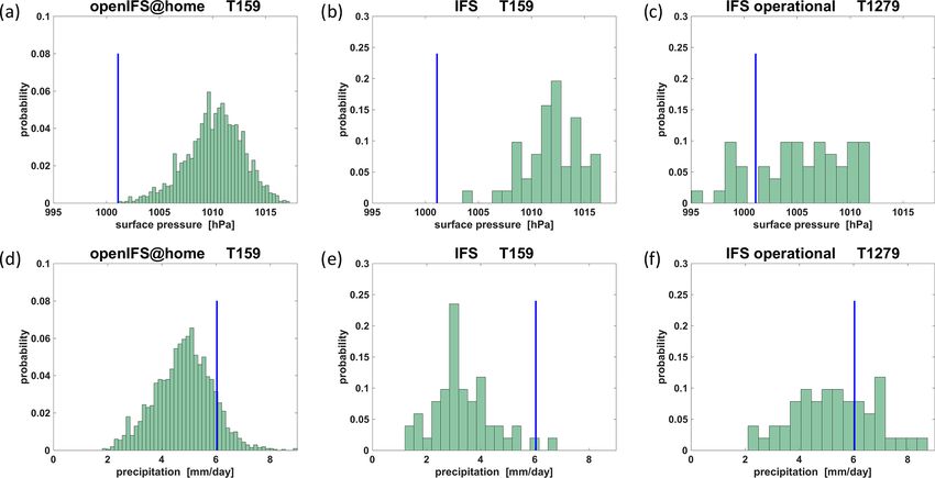
3474                                                                              S. Sparrow et al.: OpenIFS@home version 1

science project are known as volunteer or crowd computing              To increase confidence in the outcomes of large-ensemble
applications. There is an extremely wide variety of differ-         studies it is desirable to compare results across multiple
ent projects making use of this paradigm, the most well-            different models. Whilst large (on the order of 100 mem-
known of which is searching for extra-terrestrial life with         bers) ensembles can be (and are) produced by individual
SETI@home (Sullivan III et al., 1997). Projects of this type        modelling centres, this requires a great deal of coordination
are underpinned by the Berkeley Open Infrastructure for Net-        across the community on experimental design and output
work Computing (BOINC, Anderson, 2004) that distributes             variables. The computing resources required to produce very
simulations to the personal computers of their public volun-        large (> 10 000-member) ensembles are not readily available
teers that have donated their spare computing resources.            outside of citizen science projects such as CPDN. Therefore,
   For over 15 years, one such BOINC-based project, Cli-            enabling new models to work within this infrastructure to ad-
matePrediction.net (CPDN) has been harnessing public                dress questions such as those outlined above is very desir-
computing power to allow the execution of large ensem-              able.
bles of climate simulations to answer questions on uncer-              In this paper we detail the deployment of the European
tainty that would otherwise not be possible to study using          Centre for Medium-Range Weather Forecasts (ECMWF)
traditional high-performance computing (HPC) techniques             OpenIFS model within the CPDN infrastructure as the
(Allen, 1999; Stainforth et al., 2005). Volunteers can sign         OpenIFS@home application. This new facility enables the
up to CPDN through the project website and are engaged              execution of ensembles of weather forecast simulations
and retained through the mechanisms detailed in Christensen         (ranging from 1 to 10 000+ members) at scientifically rel-
et al. (2005). As well as facilitating large-ensemble climate       evant resolutions to achieve the following goals.
simulations, the project has also increased public awareness
of climate-change-related issues. Through the CPDN plat-                – To study the predictability of forecasts, especially for
form, volunteers are notified of the scientific output that they          high-impact extreme events.
have contributed towards (complete with links to the aca-
demic publication) and through the project forums and mes-              – To explore interesting past weather and climate events
sage boards can engage directly with scientists about the ex-             by testing sensitivities to physical parameter choices in
periments being undertaken. Public awareness is also raised               the model.
by press coverage of the project (e.g. “Gadgets that give
                                                                        – To help the study of probabilistic forecasts in a chaotic
back: awesome eco-innovations, from Turing Trust comput-
                                                                          atmospheric flow and reduce uncertainties due to non-
ers to the first sustainable phone” by Margolis, 2021, or
                                                                          linear interactions.
“Climate Now | Five ways you can become a citizen scien-
tist and help save the planet” by Daventry, 2020), scientific           – To support the deployment of current experiments per-
outputs (e.g. “’weather@home’ offers precise new insights                 formed with OpenIFS to run in OpenIFS@home pro-
into climate change in the West” by Oregon State Univer-                  vided certain resource constraints are met.
sity, 2016; “How your computer could reveal what’s driv-
ing record rain and heat in Australia and NZ” by Smyrk and
Minchin, 2014; “Looking, quickly, for the fingerprints of cli-      2    The ECMWF OpenIFS model
mate change” by Fountain, 2016), and through live exper-
iments undertaken directly with media outlets such as The           The OpenIFS activity at ECMWF began in 2011, with the
Guardian (Schaller et al., 2016) and British Broadcasting           objective of enabling the scientific community to use the
Corporation (BBC, Rowlands et al., 2012). To date, the anal-        ECMWF Integrated Forecast System (IFS) operational nu-
ysis performed by CPDN scientists and volunteers can be             merical weather prediction model in their own institutes for
broadly classified into three different themes. The first is cli-   research and education. OpenIFS@home as described in this
mate sensitivity analysis, where plausible ranges of climate        paper uses the OpenIFS release based on IFS cycle 40 release
sensitivity are mapped through generating large, perturbed          1, the ECMWF operational model from November 2013 to
parameter ensembles (e.g. Millar et al., 2015; Rowlands et          May 2015. The OpenIFS model differs from IFS as the data
al., 2012; Sparrow et al., 2018b; Stainforth et al., 2005; Ya-      assimilation and observation processing parts are removed
mazaki et al., 2013). The second is simulation bias reduction       from the OpenIFS model code. The forecast capability of the
methods through perturbed parameter studies (e.g. Hawkins           two models is identical, however, and the OpenIFS model
et al., 2019; Li et al., 2019; Mulholland et al., 2017). The        supports ensemble forecasts and all resolutions up to the
third category is extreme weather event attribution studies         operational resolution. OpenIFS consists of a spectral dy-
where quantitative assessments are made of the change in            namical core, a comprehensive set of physical parameteri-
likelihood of extreme weather events occurring between past,        zations, a surface model (HTESSEL), and an ocean wave
present, and possible future climates (e.g. Li et al., 2020; Otto   model (WAM). A more detailed description of OpenIFS can
et al., 2012; Philip et al., 2019; Rupp et al., 2015; Schaller et   be found in Appendix A. The relative contribution of model
al., 2016; Sparrow et al., 2018a).                                  improvements, reduction in initial state error and increased

Geosci. Model Dev., 14, 3473–3486, 2021                                              https://doi.org/10.5194/gmd-14-3473-2021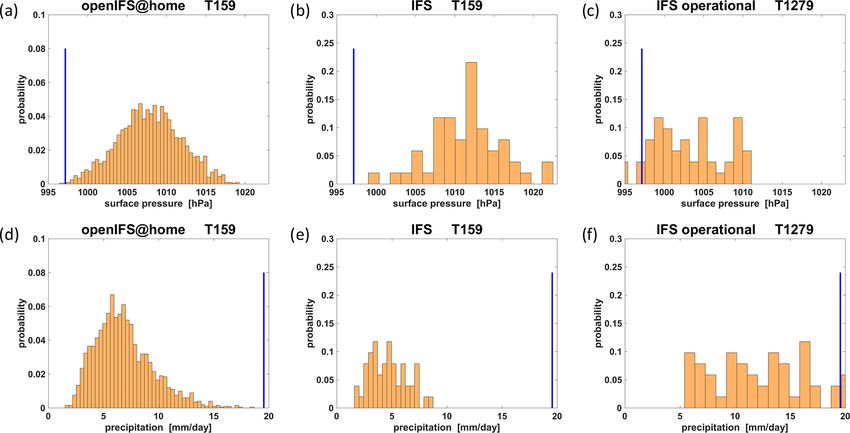
S. Sparrow et al.: OpenIFS@home version 1                                                                                         3475

use of observations to the IFS forecast performance is dis-              6. The model binary executable needs to minimize de-
cussed in detail in Magnusson and Källén (2013). A detailed                 pendencies on the specific configuration of the system
scientific and technical description of IFS can be found in                 found on the volunteer computers. Therefore, the com-
open-access scientific manuals available from the ECMWF                     pilation environment for OpenIFS@home needs to use
website (ECMWF, 2014a–d).                                                   statically linked libraries wherever possible, distributing
                                                                            these in a single application package.
3     OpenIFS@home BOINC application                                    3.2   Porting OpenIFS to a BOINC environment
3.1     Technical requirements and challenges
                                                                        To optimize OpenIFS for execution within BOINC on volun-
When creating a new volunteer computing project, there are              teer systems there are a number of changes that are required
a number of requirements for both the science team develop-             to the model beyond setup and configuration changes. The
ing it and the citizen volunteers that will execute it. As such         majority of these may be classified in terms of understand-
they can be considered boundary constraints. These are listed           ing and restricting the application footprint in terms of both
below.                                                                  overall size and resource usage during execution.
                                                                           OpenIFS is designed to work efficiently across a range
    1. The model used to build the BOINC application should             of computing systems, from massively parallel high-
       be unchanged. There are two main advantages to this.             performance computing systems to a single multi-core desk-
       First, the model itself does not require extensive reval-        top. As BOINC operates optimally if each application exe-
       idation. Second, if errors are found within the BOINC-           cution is restricted to a single core on a client system, under-
       based model, an identically configured non-BOINC                 standing and reducing memory usage becomes a priority, de-
       version may be executed locally for diagnostic pur-              termining possible resolutions the model can be executed at.
       poses. As OpenIFS is currently designed for simula-              During the initial application development, a spectral resolu-
       tion on Unix or Linux systems, initial development of            tion of T159, equivalent to a grid spacing of approximately
       OpenIFS@home has also been limited to this platform,             125 km (see the Appendix for more details of the model’s
       thereby preventing the need for a detailed revalidation.         grid structure) with 60 vertical level was chosen to ensure ex-
       Consequently, OpenIFS@home is currently limited to               ecution would complete within 1 or 2 d whilst still maintain-
       the Linux CPDN volunteer population, around 10 % of              ing satisfactory scientific performance. Typical CPDN sim-
       the 10 000 active volunteers registered with CPDN.               ulations run for considerably longer, allowing flexibility in
    2. The model configuration for an experiment and the for-           future utilization of this application.
       mulation of initial conditions and ancillary files should           Since OpenIFS@home will run on a single computer core,
       remain unchanged from that used in a standard OpenIFS            the MPI (message passing) parallel library was removed
       execution to allow easy support by the OpenIFS team in           from the OpenIFS code, though the ability to use OpenMP
       ECMWF and debugging by the CPDN.                                 was retained for possible future use. This reduces the mem-
                                                                        ory footprint and size of the binary executable.
    3. Configuration of the ensembles should be simple, re-                A model restart capability is necessary as the volunteer
       quiring minimal changes to input files to launch a large         computer may be shutdown at any point in the execution.
       batch of simulations. Web forms developed for this min-          OpenIFS provides a configurable way of enabling exact
       imize the possibility of error in the configuration.             restarts, with an option to delete older restart files. This was
                                                                        added to the model configuration to prevent excessive disk
    4. Model performance, when running on volunteers’ sys-
                                                                        use on the volunteer’s computers.
       tems, should be acceptable such that results are pro-
                                                                           There is also the requirement to transfer to volunteer sys-
       duced at a useful frequency for the submitting re-
                                                                        tems the configuration files that control the execution of the
       searcher and so that the time to completion of an in-
                                                                        model and the return of model output files. The design of
       dividual simulation workunit is practical for the volun-
                                                                        OpenIFS makes it inherently suitable for deployment under
       teers’ systems. This dictates the resolution of the simu-
                                                                        BOINC. Input and output files use the standard GRIB for-
       lation that can be run; a lower resolution than that uti-
                                                                        mat (World Meteorological Organization (WMO), 2003) that
       lized operationally, but one that is still scientifically use-
                                                                        was originally designed for transmission over slow telecom-
       ful.
                                                                        munication lines. The model output files are separated into
    5. The model must not generate excessive volumes of out-            spectral and grid point fields. Each model level of each field
       put data such that volunteers’ network connections are           is encoded in a self-describing format, whilst the field data
       overwhelmed. This requires integration of existing mea-          itself is packed into a specified “lossy” bit precision. This
       sures to analyse the model configuration so that the             greatly reduces the amount of data transmission, whilst the
       CPDN team can validate the expected data volumes be-             self-describing nature of each of the GRIB fields supports a
       fore submission.                                                 “trickle” of output results as the model runs. Scientists are

https://doi.org/10.5194/gmd-14-3473-2021                                                  Geosci. Model Dev., 14, 3473–3486, 2021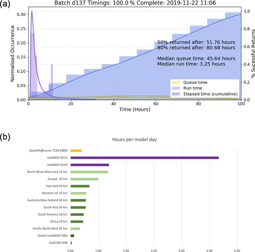
3476                                                                                S. Sparrow et al.: OpenIFS@home version 1

Figure 1. Evolution of Tropical Cyclone Karl on 27 and 28 September 2016 showing the downstream impact with heavy rainfall over western
Norway. Contour lines display mean sea level pressure (hPa) from the ECMWF operational analysis. Colour shading shows the 12-hourly
accumulated total precipitation (mm) from the ECMWF operational forecast.

expected to carefully choose the model fields and levels re-          4     Demonstration
quired to minimize output file sizes and transmission times
to the CPDN servers. This is an optimization exercise that            4.1    Case study: Tropical Cyclone Karl
is supported by CPDN, with exact thresholds depending on
frequency of return as well as absolute file size due to differ-      Recent research into mid-latitude weather predictability has
ences in volunteer’s internet connectivity.                           focused on the role of diabatic processes. Research flight
   The GRIB-1 and GRIB-2 definitions do, however, intro-              campaigns provide in situ measurements of diabatic and
duce one difficulty. The encoding of the ensemble member              other physical processes against which models can be vali-
number only supports values up to 255. To overcome this,              dated. The NAWDEX flight campaign (Schäfler et al., 2018)
custom changes were made to the output GRIB files to al-              focused on weather features associated with forecast errors,
low exploitation of the much larger ensembles that could be           for example the poleward recurving of tropical cyclones,
distributed within OpenIFS@home. Specifically, four spare             which is known to be associated with low predictability (Harr
bytes in the output grid point GRIB fields were used to cre-          et al., 2008). To demonstrate the new OpenIFS@home fa-
ate a custom ensemble perturbation number (defined in local           cility, we simulated the later development of a tropical cy-
part of section 1 in GRIB-1 output; section 3 of GRIB-2 out-          clone (TC) in the North Atlantic that occurred during the
put). The custom GRIB templates must be distributed with              NAWDEX campaign. In September 2016, TC Karl under-
the model to the volunteer’s computer and subsequently used           went extratropical transition and its path moved far into the
when decoding the returned GRIB output files.                         mid-latitudes. The storm resulted in high-impact weather in
                                                                      north-western Europe (Euler et al., 2019). After leaving the
                                                                      subtropics on 25 September, ex-TC Karl moved northwards
                                                                      and merged with a weak pre-existing cyclone. This resulted
                                                                      in rapid intensification and the formation of an unusually

Geosci. Model Dev., 14, 3473–3486, 2021                                                https://doi.org/10.5194/gmd-14-3473-2021
S. Sparrow et al.: OpenIFS@home version 1 3477
strong jet streak downstream near Scotland 2 d later. This ini- Lang, 2014). The Stochastically Perturbed Parameterization
tiated further development with heavy and persistent rainfall Tendencies (SPPT) scheme (Buizza et al., 2007; Palmer et
over western Norway. al., 2009; Shutts et al., 2011) was used on top of the initial
state perturbations to represent model error in the ensemble.
4.2 Experimental setup and initial conditions The results from this experiment were compared against
output from an ensemble of the same size as ECMWF’s op-
A 6 d forecast experiment was designed to capture the ex- erational forecasts (51 members) run at the same horizontal
tratropical transition of TC Karl and the associated high im- resolution as our forecast experiment using the current oper-
pact weather north of Scotland and near the Norwegian west ational IFS cycle at the time of writing (CY46R1).
coast. The forecasts were initialized on 25 September 2016
at 00:00 UTC (see Fig. 1). The wave model was switched 4.3 Performance
off in OpenIFS for this experiment. Compared to the op-
erational forecasting system at ECMWF and other major 4.3.1 BOINC application performance
weather centres, the OpenIFS grid resolution used here is
coarse (∼ 125 km grid spacing) and hence the model’s abil- Figure 2a shows the behaviour of the batch of simulations
ity to resolve orographic effects over smaller scales will be (OpenIFS@home dashboard, ClimatePrediction.net, 2019),
limited. detailing how long simulations were in the queue (yellow),
To represent the uncertainty in the initial conditions and to took to run (purple), and took to accumulate an ensemble
evaluate the range of possible forecasts, a 2000-member en- of successful results (blue). The overall percentage of suc-
semble with perturbed initial conditions was launched. The cessfully completed runs in the batch compared to those dis-
ECMWF data assimilation system was used to create 250 tributed is also shown in the title. Medians rather than means
perturbed initial states. Each of these 250 states was then are quoted as distributions can have long tails. This is due to
used for eight forecasts in the 2000-member ensemble. A dif- the nature of the computing resources used, where for a va-
ferent forecast realisation for each set of eight forecasts was riety of reasons a small number of simulations (work units)
generated by enabling the stochastic noise in the OpenIFS may go to systems that may not run or connect to the internet
physical parameterizations. for a non-trivial period after receiving work. This validation
The initial-state perturbations in the ECMWF operational batch was run on the CPDN development site where fewer
IFS ensemble are generated by combining so-called singu- systems are connected than on the main site, but they are
lar vectors (SVs) with an ensemble of data assimilations more likely to be running continuously. The median queue
(EDA) (Buizza et al., 2008; Isaksen et al., 2010; Lang et time was 45.64 h, and the 6 d simulations had a median run-
al., 2015). The SVs represent atmospheric modes that grow time of 3.25 h across the different volunteer machines. Half
rapidly when perturbed from the default state. In the opera- of the batch (i.e. 50 % of the ensemble) was returned af-
tional IFS ensemble, the modes that result in maximum total ter 51.76 h with 80 % completion (the criteria typically cho-
energy deviations in a 48 h forecast lead time are targeted. sen for closure of a batch) being achieved after 80.68 h.
A total of 50 of these modes are searched for in the North- The median run time distribution (purple) shows a bi-modal
ern Hemisphere, 50 are searched for in the Southern Hemi- structure that reflects the different system specifications and
sphere, and 5 modes per active tropical cyclone are searched project connectivity of client machines connected to the de-
for in the tropics. The final SV initial-state perturbation fields velopment site. As detailed in Anderson (2004) and Chris-
are constructed as a linear combination of the found SVs tensen et al. (2005), each volunteer can configure their own
(Leutbecher and Palmer, 2008). The EDA-based perturba- project connectivity and available resources as well as spec-
tions, on the other hand, try to assess uncertainties in the ify during which times their system can be used to compute
observations (and the model itself) used in the data assim- work, and thus these timings should be viewed as indica-
ilation (DA). This is achieved by running the IFS DA at a tive rather than definitive. Figure 2b shows how the run time
lower resolution multiple times and applying perturbations from a representative batch of OpenIFS@home simulations
to the used observations and the model physics. In the oper- compares to the other UK Met Office model configurations
ational IFS ensemble, 50 of these DA cycles are run (Lang available on the CPDN platform (although typically these
et al., 2019). The final perturbation fields that the operational are used to address different questions) and demonstrates
IFS ensemble uses are a combination of both of the perturbed that not only is the OpenIFS@home run time comparable to
fields. Here, we apply the same methodology as in the oper- the different embedded regional models in weather@home,
ational IFS ensemble initialization. The only differences are it is also among the faster running models on the platform.
that (i) the used model version and resolution differ from the The OpenIFS@home application running at this resolution
operational setup, (ii) only 25 DA cycles are run with a ± (T159L60) requires 3.2 Gb of storage and 5.37 Gb of random
symmetry to construct 50 initial states, and (iii) we calcu- access memory (RAM).
late 250 SV modes in the extra-tropics, instead of the default Although individual simulations will not necessarily be bit
50. This was motivated by the discussion in (Leutbecher and reproducible when run on systems with different operating
https://doi.org/10.5194/gmd-14-3473-2021 Geosci. Model Dev., 14, 3473–3486, 20213478 S. Sparrow et al.: OpenIFS@home version 1
Figure 2. (a) The relevant timings associated with the validation batch. The queue time (yellow) and run time (purple) distributions are
straight occurrence distributions, whereas the elapsed time (blue) is a cumulative distribution expressed as a percentage of the successful
returns. (b) Run time information in hours per model day based on a representative batch for applications on the CPDN platform (note these
numbers are indicative rather than definitive). ECMWF OpenIFS@home is depicted in yellow, UK Met Office weather@home (HadAM3P
with various HadRM3P regions) configurations are depicted in green (with light green indicating a 25 km embedded region, green indicating
a 50 km embedded region, and dark green indicating where only the global driving model is computed). The UK Met Office low-resolution
coupled atmosphere–ocean model HadCM3 is shown in blue, and the high-resolution global atmosphere HadAM4 at N144 (∼ 90 km mid-
latitudes) and N216 (∼ 60 km mid-latitudes) are shown in purple.
systems and processor types. Knight et al. (2007) demon-
strate the effect of hardware and software is small relative
to the effect of parameter variation and can be considered
equivalent to those differences caused by changes in initial
conditions. Given the large ensembles involved, the proper-
ties of the distributions themselves are not expected to be
affected by different mixes of hardware in computing indi-
vidual ensemble members.
4.3.2 Meteorological performance
TC Karl, as it moved eastward across the North Atlantic, was
associated with a band of low surface pressure that reached
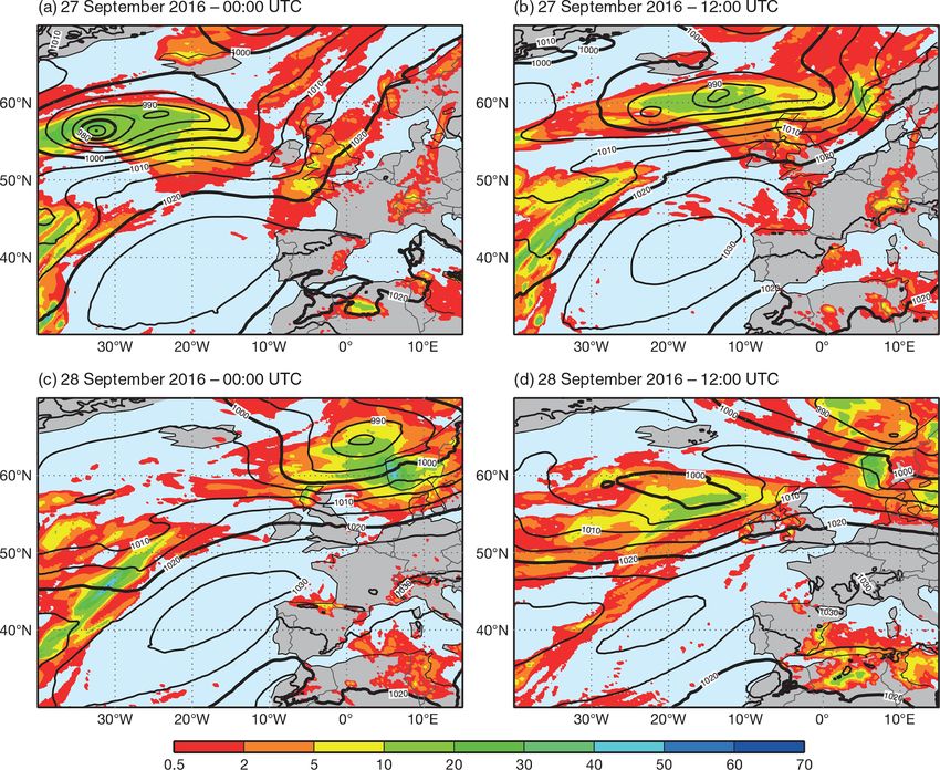
Figure 3. Two regions over northern Scotland (green) and around over a region of northern Scotland 60 h into the forecasts and
Bergen (orange) that have been used in the diagnostics of the model near Bergen on the coast of Norway at 72 h (see green and
performance.
orange boxes in Fig. 3 for the regions).
Geosci. Model Dev., 14, 3473–3486, 2021 https://doi.org/10.5194/gmd-14-3473-2021S. Sparrow et al.: OpenIFS@home version 1 3479 Figure 4. Ensemble forecast distribution in northern Scotland of mean sea level pressure (a–c) and total precipitation (d–f) in the OpenIFS@home ensemble (a, d), in the IFS experiment (b, e), and in the operational forecast (c, f). The vertical blue line indicates the verification as derived from ECMWF’s analysis. Mean sea level pressure data are for a 60 h forecast lead time. Total precipitation data are accumulated between forecast lead times of 60 to 72 h. We discuss here the results of the OpenIFS@home fore- ample, the operational high-resolution ECMWF forecast is cast using 2000 ensemble members run at a horizontal res- shown in Fig. 4c. The distribution is nearly uniformly dis- olution of approx. 125 km (the T159 spectral resolution). tributed between 999 and 1012 hPa. The analysis value lies These forecasts will be contrasted with two 51-ensemble well within that range, though interestingly it is at a local member forecasts of the IFS run on the ECMWF supercom- minimum of the distribution. With the application of suitable puter: a low-resolution experiment also at 125 km (T159) calibration or adjustment for the horizontal model resolution- resolution and the operational forecast at the time of TC dependent underestimation bias in the surface pressure mean, Karl, which has a resolution of approx. 18 km (T1279) that the example of TC Karl demonstrates the power of large is almost an order of magnitude finer. ECMWF’s operational ensembles to assign non-zero probabilities to extreme out- weather forecasts are comprised of 51 individual ensemble comes at the very tails of the distribution members and serves here as a benchmark. The precipitation forecasts for northern Scotland are The OpenIFS@home ensemble predicted a distribution of shown in Fig. 4d–f. OpenIFS@home forecasts a substantial surface pressure averaged over the northern Scotland area probability to the possibilities of rainfall values larger than with a mean of approx. 1011 hPa and a long tail towards the analysis. A traditional-sized ensemble of the same hori- low-pressure values (Fig. 4a). The analysis value of 1001 hPa zontal resolution considers the observed outcome much less is just at the lowest edge of the distribution, indicating that likely than the large OpenIFS@home ensemble. The high- while the OpenIFS@home model was able to assign a non- resolution forecast at operational resolution arguably did not zero probability to this extreme outcome, it did not indicate a perform much better than OpenIFS@home even though the seriously large risk for such small values. In comparison, the low-pressure system itself would be better simulated. forecast with the standard operational prediction ensemble The forecasts of surface pressure and precipitation over size of 51 members (Fig. 4b) did not even include the ob- the region near Bergen are shown in Fig. 5. Similar to served minimum in its tails, implying that the observed event the performance north of Scotland, the large ensemble of was virtually impossible to occur. This clearly demonstrates OpenIFS@home (Fig. 5a) does include in its distribution the power of our large ensemble which, while not assigning a the observed low-pressure value, while in the case of a 51- significant probability to the observed outcome, did include member IFS T159 ensemble even the lowest forecast value it as a possible though unlikely outcome. The overestimation was above the analysis (Fig. 5b). The high-resolution opera- of the surface pressure in the OpenIFS@home forecasts is tional IFS forecast (Fig. 5c) gave a higher probability to the hardly surprising because the magnitude of pressure minima observed outcome than OpenIFS@home but also considered strongly depends on the horizontal model resolution. For ex- it extreme within its predicted range. https://doi.org/10.5194/gmd-14-3473-2021 Geosci. Model Dev., 14, 3473–3486, 2021
3480                                                                                       S. Sparrow et al.: OpenIFS@home version 1

Figure 5. Ensemble forecast distribution near Bergen of mean sea level pressure (a–c) and total precipitation (d–f) in the OpenIFS@home
ensemble (a, d), in the IFS experiment (b, e), and in the operational forecast (c, f). The vertical blue line indicates the verification as derived
from ECMWF’s analysis. Mean sea-level pressure data are for a 72 h forecast lead time. Total precipitation data are accumulated between
forecast lead times of 60 and 72 h.

   The extreme precipitation amount of nearly 20 mm d−1                     events. For these situations, the availability of very large en-
in the analysis for the region around Bergen was only cap-                  sembles that enable a meaningful sampling of the tails of the
tured by the high-resolution operational IFS forecast (Fig. 5f)             distribution, and with it the risks for extreme outcomes, will
which is likely a result of the much improved representation                be most valuable. Our TC Karl analysis has made that point
of the small-scale orography over the coast of Norway in                    very clear by showing a substantial improvement in the prob-
runs with high horizontal resolution, with implications for                 abilistic forecasts of both very low surface pressure (and as-
orographic rain amounts. While the entire distribution of the               sociated winds) and large rainfall totals.
51-member IFS ensemble was far off the observed amount
without any indication of possibly more extreme outcomes
(Fig. 5e), the large ensemble of OpenIFS@home (Fig. 5d)                     5   Conclusions
produced a long tail towards extreme precipitation amounts
which nearly reached 20 mm d−1 .                                            This paper introduced the OpenIFS@home project (ver-
   The forecast accuracy of the extreme meteorological con-                 sion 1) that enables the production of very large ensem-
ditions of TC Karl is influenced by three key factors: (i) a                ble weather forecasts, supporting types of studies previ-
good physical model that can simulate the atmospheric flow                  ously too computationally expensive to attempt and grow-
in highly baroclinic extratropical conditions as an extratrop-              ing the research community able to access OpenIFS. This
ical low-pressure system; (ii) a higher horizontal resolution               was completed with the help of citizen scientists who vol-
that allows a better resolution of the storm, and (iii) a large             unteered computational resources and the deployment of the
ensemble that samples a wide range of uncertainties given                   ECMWF OpenIFS model within the CPDN infrastructure as
the simulated flow for a given resolution. OpenIFS@home                     the OpenIFS@home application. The work is based on the
is built on the world-leading Numerical Weather Prediction                  ClimatePrediction.net and weather@home systems enabling
(NWP) forecast model of ECMWF that enables our dis-                         a simpler and more sustainable deployment.
tributed forecasting system to use the most advanced science                   We validated the first use of OpenIFS@home in a volun-
of weather prediction. Arguably, a storm like Karl will be                  teer computing framework for ensemble forecast simulations
better resolved with higher horizontal resolution, as becomes               using the example of TC Karl (September 2016) over the
clear in our demonstration of the IFS performance in two                    North Atlantic. Forecasts with 2000 ensemble members were
contrasting resolutions. However, there are other meteoro-                  generated for 6 d ahead and computed by volunteers within
logical phenomena where horizontal resolution does not play                 ∼ 3 d. Significantly smoother probability distribution can be
a similarly large role in the successful prediction of extreme              created than forecasts generated with significantly fewer en-

Geosci. Model Dev., 14, 3473–3486, 2021                                                        https://doi.org/10.5194/gmd-14-3473-2021
S. Sparrow et al.: OpenIFS@home version 1                                                                                     3481

semble members. In addition, the very large ensemble can             We have demonstrated that the current application as de-
represent the uncertainty better, particularly in the tails of    ployed produces scientifically relevant results within a useful
the forecast distributions, allowing higher accuracy of the       time frame, whilst utilizing acceptable amounts of computa-
probability of extremes of the forecast distribution. The rel-    tional resources on volunteering citizen scientist’s personal
atively low horizontal resolution of OpenIFS@home when            computers. However, further developments have been identi-
compared with typical operational NWP resolutions and the         fied as desirable in the future use of the facility. For instance,
potential implications due to the resolution are, however, a      developing a working application for Windows (and Ma-
limitation that always must be kept in mind for specific appli-   cOS) systems would significantly increase the number of vol-
cations. This system has significant future potential and of-     unteers available to compute OpenIFS@home simulations,
fers opportunities to address topical scientific investigation,   which in turn would result in a reduction in queue time for
some of examples of which are listed below.                       simulations and engage public volunteers from a wider com-
                                                                  munity. Another possible future development will look at uti-
  – Performing comprehensive sensitivity analyses to at-          lizing multiple cores via the OpenMP multi-threading capa-
    tribute sources of uncertainty, which dominate the mete-      bility of OpenIFS. As new versions of the OpenIFS model
    orological forecasts and meteorological analyses direct-      are released, the OpenIFS@Home facility will be updated as
    ing where to allocate resources for future research, i.e.     resources allow.
    understanding how much meteorological uncertainty is             In terms of potential areas of future scientific use of
    generated through the land surface parameterization in        openIFS@home, research on understanding and predicting
    comparison to the ocean.                                      compound extreme events (for example, a heat wave in con-
  – Investigating the tails of distribution and forecast out-     junction with a meteorological and hydrological drought)
    liers which are important for risk-based decision-            will be of interest. ECMWF’s operation ensemble size of
    making, particularly in high-impact, low-probability          51 members makes such investigations very difficult and
    scenarios, e.g. tropical cyclone landfall.                    limited in their scope, while the very large ensemble setup
                                                                  of openIFS@home provides an ideal framework for the re-
  – Improving the understanding of non-linear interactions        quired sample sizes of multivariate studies. We are plan-
    of all Earth system components and their uncertainties        ning to use the system for predictability research on a range
    will provide valuable insight into fundamental model          of timescales from days to weeks and months, with poten-
    processes. Not only will large initial conditions ensem-      tial idealized climate applications also feasible in the longer
    bles be possible but so will large multi-model perturbed      term.
    parameter experiments.

https://doi.org/10.5194/gmd-14-3473-2021                                             Geosci. Model Dev., 14, 3473–3486, 2021
3482 S. Sparrow et al.: OpenIFS@home version 1
Appendix A: OpenIFS description senting deep, shallow, and mid-level convection (Bechtold et
al., 2008; Tiedtke, 1989), with a recent update to the convec-
OpenIFS uses a hydrostatic dynamical core for all fore- tive closure for significant improvements in the convective
cast resolutions, with prognostic equations for the horizon- diurnal cycle (Bechtold et al., 2014). The cloud scheme is
tal wind components (vorticity and divergence), temperature, based on Tiedtke (1993) but with an enhanced representation
water vapour, and surface pressure. The hydrostatic, shallow- of mixed-phase clouds and prognostic precipitation (Forbes
atmosphere approximation primitive equations are solved us- and Tompkins, 2011; Forbes et al., 2011). The HTESSEL
ing a two-time-level, semi-implicit semi-Lagrangian formu- tiled surface scheme represents the surface fluxes of energy
lation (Hortal, 2002; Ritchie et al., 1995; Staniforth and Côté, and water and the corresponding sub-surface quantities. Sur-
1991; Temperton et al., 2001). OpenIFS is a global model face sub-grid types of vegetation, bare soil, snow, and open
and does not have the capability for limited-area forecasts. water are represented (Balsamo et al., 2009). Unresolved oro-
The dynamical core is based on the spectral transform graphic effects are parameterized according to Beljaars et
method (Orszag, 1970; Temperton, 1991). Fast Fourier trans- al. (2004) and Lott and Miller (1997). Non-orographic grav-
forms (FFTs) in the zonal direction and Legendre transforms ity waves are parameterized according to Orr et al. (2010).
(LT) in the meridional direction are used to transform the The sea surface has a two-way coupling to the ECMWF
representation of variables to and from grid point to spec- wave model (Janssen, 2004). Monthly mean climatologies
tral space. The spectral representation is used to compute for aerosols, long-lived trace gases, and surface fields such
horizontal derivatives, efficiently solve the Helmholtz equa- as sea surface temperature are read from external fields pro-
tion associated with the semi-implicit time-stepping scheme, vided with the model package. Although IFS includes an
and apply horizontal diffusion. The computation of semi- ocean model for operational forecasts, OpenIFS does not in-
Lagrangian horizontal advection, the physical parameteriza- clude it.
tions, and the non-linear right-hand-side terms are all com- In order to represent random model error due to un-
puted in grid point space. The horizontal resolution is there- resolved sub-grid-scale processes, OpenIFS includes the
fore represented by both the spectral truncation wavenumber stochastic parameterization schemes of IFS (see Leutbecher
(the number of retained waves in spectral space) and the res- et al., 2017, for an overview). For example, the SPPT scheme
olution of the associated Gaussian grid. Gaussian grids are perturbs the total tendencies from all physical parameteriza-
regular in longitude but slightly irregular in latitude with no tions using a multiplicative noise term (Buizza et al., 2007;
polar points. Model resolutions are usually described using Palmer et al., 2009; Shutts et al., 2011).
a Txxx notation where xxx is the number of retained waves
in spectral representation. In the vertical, a hybrid sigma–
pressure-based coordinate is used, in which the lowest lay-
ers are pure so-called “sigma” levels, whilst the topmost
model levels are pure pressure levels (Simmons and Bur-
ridge, 1981). The vertical resolution varies smoothly with ge-
ometric height and is finest in the planetary boundary layer,
becoming coarser towards the model top. A finite-element
scheme is used for the vertical discretization (Untch and Hor-
tal, 2004). In this paper, all OpenIFS@home forecasts used
the T159 horizontal resolution on a linear model grid with 60
vertical levels. This approximates to a resolution of 125 km
at the Equator or a “N80” grid.
The OpenIFS model includes a comprehensive set of sub-
grid parameterizations representing radiative transfer, con-
vection, clouds, surface exchange, turbulent mixing, sub-
grid-scale orographic drag, and non-orographic gravity wave
drag. The radiation scheme uses the Rapid Radiation Trans-
fer Model (RRTM) (Mlawer et al., 1997) with cloud radi-
ation interactions using the Monte Carlo Independent Col-
umn Approximation (McICA) (Morcrette et al., 2008). Ra-
diation calculations of short- and long-wave radiative fluxes
are done less frequently than the time step of the model
and on a coarser grid. This is relevant for implementation in
the BOINC framework because this calculation of the fluxes
represents the high-water memory usage of the model. The
moist convection scheme uses a mass-flux approach repre-
Geosci. Model Dev., 14, 3473–3486, 2021 https://doi.org/10.5194/gmd-14-3473-2021S. Sparrow et al.: OpenIFS@home version 1 3483
Code availability. The BOINC implementation of OpenIFS, as dis- OpenIFS@home; developed web interfaces for generating ensem-
tributed by CPDN, includes a free personal binary-only license to bles, managing ancillary data files, and monitoring distribution
use the custom OpenIFS binary executable on the volunteer com- of ensembles; and wrote the training documentation. AB devel-
puter. Researchers who need to modify the OpenIFS source code oped the BOINC application for OpenIFS@home that is dis-
for use in OpenIFS@home must have an OpenIFS software source tributed to client machines and wrote scripts for submission of
code license. OpenIFS@home ensembles into the CPDN system. GDC devel-
A software licensing agreement with ECMWF is required to ac- oped the BOINC version of OpenIFS deployed in OpenIFS@home.
cess the OpenIFS source distribution: despite the name it is not MOK contributed to the preparation of the experiment initial con-
provided under any form of open-source software license. License ditions. PO generated the perturbed initial states. DW was influen-
agreements are free, limited to non-commercial use, forbid any real- tial in specifying the overall concept and the specific BOINC ap-
time forecasting, and must be signed by research or educational plication design of OpenIFS@home. FP was influential in the de-
organizations. Personal licenses are not provided. OpenIFS can- velopment of OpenIFS@home. AW was instrumental in the con-
not be used to produce or disseminate real-time forecast products. ceptual idea of using OpenIFS as a state-of-the-art weather predic-
ECMWF has limited resources to provide support and thus may tion model for citizen science large-ensemble simulations. AW also
temporarily cease issuing new licenses if it is deemed too difficult developed some of the diagnostics. All authors contributed to the
to provide a satisfactory level of support. Provision of an OpenIFS writing of the manuscript.
software license does not include access to ECMWF computers or
data archives other than public datasets.
OpenIFS requires a version of the ECMWF ecCodes GRIB li- Competing interests. The authors declare that they have no conflict
brary for input and output: version 2.7.3 was used in this paper of interest.
(though results are not dependent on the version). All required ec-
Codes files, such as the modified GRIB templates, are included
in the application tarfile available from Centre for Environmen- Acknowledgements. We gratefully acknowledge the personal com-
tal Data Analysis (http://www.ceda.ac.uk, last access: 1 June 2021, puting time given by the CPDN moderators for this project. We
see data availability section below for details). Version 2.7.3 of ec- are grateful for the assistance provided by ECMWF for solving the
Codes can also be downloaded from the ECMWF GitHub reposi- GRIB encoding issue for very large ensemble member numbers.
tory (https://github.com/ecmwf, last access: 1 June 2021, ECMWF,
2021), though note that the modified GRIB templates included in
the application tarfile must be used.
Review statement. This paper was edited by Volker Grewe and re-
Parties interested in modifying the model source code should
viewed by Wilco Hazeleger and Thomas M. Hamill.
contact ECMWF, by emailing openifs-support@ecmwf.int, to re-
quest a license outlining their proposed use of the model. Consid-
eration may be given to requests that are judged to be beneficial for
future ECMWF scientific research plans or those from scientists in- References
volved in new or existing collaborations involving ECMWF. See the
following webpage for more details: https://software.ecmwf.int/oifs Allen, M.: Do-it-yourself climate prediction, Nature, 401, 642,
(last access: 1 June 2021). https://doi.org/10.1038/44266, 1999.
All bespoke code that has been produced in the creation of Anderson, D. P.: BOINC: A system for public-resource com-
OpenIFS@home is kept in a set of publicly available open-source puting and storage, in: GRID ’04: Proceedings of the 5th
GitHub repositories under the CPDN-Git organization (https:// IEEE/ACM International Workshop on Grid Computing, 4–10,
github.com/CPDN-git, last access: 1 June 2021). The exact release https://doi.org/10.1109/GRID.2004.14, 2004.
versions (1.0.0) are archived on Zenodo (Bowery and Carver 2020; Balsamo, G., Viterbo, P., Beijaars, A., van den Hurk, B., Hirschi,
Sparrow, 2020a–c; Uhe and Sparrow, 2020). M., Betts, A. K., and Scipal, K.: A revised hydrology for the
The OpenIFS@home binary application code version 2.19, to- ECMWF model: Verification from field site to terrestrial water
gether with the post-processing and plotting scripts used to analyse storage and impact in the integrated forecast system, J. Hydrom-
and produce the figures in this paper, are included within the deposit eteorol. 10, 623–643, https://doi.org/10.1175/2008JHM1068.1,
at the CEDA data archive (details provided in the data availability 2009.
section). Bechtold, P., Köhler, M., Jung, T., Doblas-Reyes, F., Leutbecher,
M., Rodwell, M. J., Vitart, F., and Balsamo, G.: Advances in sim-
ulating atmospheric variability with the ECMWF model: From
Data availability. The initial conditions used for the Tropical Cy- synoptic to decadal time-scales, Q. J. Roy. Meteor. Soc., 134,
clone Karl forecasts described in this paper, together with the full 1337–1351, https://doi.org/10.1002/qj.289, 2008.
set of model output data for the experiment used in this study, are Bechtold, P., Semane, N., Lopez, P., Chaboureau, J. P., Beljaars, A.,
freely available (Sparrow et al., 2021) at the Centre for Environmen- and Bormann, N.: Representing equilibrium and nonequilibrium
tal Data Analysis (http://www.ceda.ac.uk, last access: 1 June 2021). convection in large-scale models, J. Atmos. Sci., 71, 734–753,
https://doi.org/10.1175/JAS-D-13-0163.1, 2014.
Beljaars, A. C. M., Brown, A. R., and Wood, N.: A new
parametrization of turbulent orographic form drag, Q. J. Roy.
Author contributions. SS was instrumental in specifying over-
Meteor. Soc., 130, 1327–1347, https://doi.org/10.1256/qj.03.73,
all concept as well as the BOINC application design for
2004.
https://doi.org/10.5194/gmd-14-3473-2021 Geosci. Model Dev., 14, 3473–3486, 20213484 S. Sparrow et al.: OpenIFS@home version 1 Bowery, A. and Carver, G.: Instructions and code for controlling Hawkins, L. R., Rupp, D. E., McNeall, D. J., Li, S., Betts, R. A., ECMWF OpenIFS application in ClimatePrediction.net (CPDN) Mote, P. W., Sparrow, S. N., and Wallom, D. C. H.: Parametric [code],=, Zenodo, https://doi.org/10.5281/zenodo.3999557, Sensitivity of Vegetation Dynamics in the TRIFFID Model and 2020. the Associated Uncertainty in Projected Climate Change Impacts Buizza, R., Milleer, M., and Palmer, T. N.: Stochastic represen- on Western U.S. Forests, J. Adv. Model. Earth Sy., 11, 2787– tation of model uncertainties in the ECMWF ensemble pre- 2813, https://doi.org/10.1029/2018MS001577, 2019. diction system, Q. J. Roy. Meteor. Soc., 125, 2887–2908, Hortal, M.: The development and testing of a new two-time- https://doi.org/10.1002/qj.49712556006, 2007. level semi-Lagrangian scheme (SETTLS) in the ECMWF Buizza, R., Leutbecher, M., and Isaksen, L.: Potential use of forecast model, Q. J. Roy. Meteor. Soc., 128, 1671–1687, an ensemble of analyses in the ECMWF Ensemble Pre- https://doi.org/10.1002/qj.200212858314, 2002. diction System, Q. J. Roy. Meteor. Soc., 134, 2051–2066, Isaksen, L., Bonavita, M., Buizza, R., Fisher, M., Haseler, J., Leut- https://doi.org/10.1002/qj.346, 2008. becher, M., and Raynaud, L.: Ensemble of data assimilations at Christensen, C., Aina, T., and Stainforth, D.: The challenge of vol- ECMWF, ECMWF Technical Memoranda No. 636, ECMWF, unteer computing with lengthy climate model simulations, Pro- https://doi.org/10.21957/obke4k60, 2010. ceedings of the 1st IEEE Conference on e-Science and Grid Janssen, P. A. E. M.: The Interaction of Ocean Waves and Wind, Computing, Melbourne, Australia, 5–8 December 2005. Cambridge University Press, 385 pp., 2004. ClimatePrediction.net: OpenIFS@home dashboard, available at: Knight, C. G., Knight, S. H. E., Massey, N., Aina, T., Christensen, https://dev.cpdn.org/oifs_dashboard.php (last access: 29 June C., Frame, D. J., Kettleborough, J. A., Martin, A., Pascoe, S., 2020), 2019. Sanderson, B., Stainforth, D. A., and Allen, M. R.: Association Daventry, M.: Climate Now | Five ways you can become a cit- of parameter, software, and hardware variation with large-scale izen scientist and help save the planet, EuroNews, available behavior across 57,000 climate models, P. Natl. Acad. Sci. USA, at: https://www.euronews.com/2020/12/17/climate-now-how-to- 104, 12259–12264, https://doi.org/10.1073/pnas.0608144104, become-a-citizen-scientist-and-help-‚save-the-planet (last ac- 2007. cess: 25 January 2021), 2020. Lang, S. T. K., Bonavita, M., and Leutbecher, M.: On the impact of ECMWF: IFS Documentation CY40R1 – Part III: re-centring initial conditions for ensemble forecasts, Q. J. Roy. Dynamics and Numerical Procedures, ECMWF, Meteor. Soc., 141, 2571–2581, https://doi.org/10.1002/qj.2543, https://doi.org/10.21957/khi5o80, 2014a. 2015. ECMWF: IFS Documentation CY40R1 – Part IV: Physical Pro- Lang, S., Hólm, E., Bonavita, M., and Tremolet, Y.: A 50-member cesses, ECMWF, https://doi.org/10.21957/f56vvey1x, 2014b. Ensemble of Data Assimilations, ECMWF Newsletter No. 158, ECMWF: IFS Documentation CY40R1 – Part VI: 27–29, https://doi.org/10.21957/nb251xc4sl, 2019. Technical and computational procedures, ECMWF, Leutbecher, M. and Lang, S. T. K.: On the reliability of ensem- https://doi.org/10.21957/l9d0p4edi, 2014c. ble variance in subspaces defined by singular vectors, Q. J. Roy. ECMWF: IFS Documentation CY40R1 – Part VII: ECMWF Wave Meteor. Soc., 140, 1453–1466, https://doi.org/10.1002/qj.2229, Model, ECMWF, https://doi.org/10.21957/jp6ffnj, 2014d. 2014. ECMWF: ECMWF GitHub repository, available at: https://github. Leutbecher, M. and Palmer, T. N.: Ensemble fore- com/ecmwf, last access: 1 June 2021, casting, J. Comput. Phys., 227, 3515–3539, Euler, C., Riemer, M., Kremer, T., and Schömer, E.: Lagrangian https://doi.org/10.1016/j.jcp.2007.02.014, 2008. description of air masses associated with latent heat release in Leutbecher, M., Lock, S. J., Ollinaho, P., Lang, S. T. K., Balsamo, tropical Storm Karl (2016) during extratropical transition, Mon. G., Bechtold, P., Bonavita, M., Christensen, H. M., Diamantakis, Weather Rev., 147, 2657–2676, https://doi.org/10.1175/MWR- M., Dutra, E., English, S., Fisher, M., Forbes, R. M., Goddard, D-18-0422.1, 2019. J., Haiden, T., Hogan, R. J., Juricke, S., Lawrence, H., MacLeod, Forbes, R. and Tompkins, A.: An improved representation of D., Magnusson, L., Malardel, S., Massart, S., Sandu, I., Smo- cloud and precipitation, ECMWF Newsletter No. 129, 13–18, larkiewicz, P. K., Subramanian, A., Vitart, F., Wedi, N., and https://doi.org/10.21957/nfgulzhe, 2011. Weisheimer, A.: Stochastic representations of model uncertain- Forbes, R. M., Tompkins, A. M., and Untch, A.: A new prognostic ties at ECMWF: state of the art and future vision, Q. J. Roy. bulk microphysics scheme for the IFS, ECMWF Technical Mem- Meteor. Soc., 143, 2315–2339, https://doi.org/10.1002/qj.3094, orandum No. 649, 22 pp., https://doi.org/10.21957/bf6vjvxk, 2017. 2011. Li, S., Rupp, D. E., Hawkins, L., Mote, P. W., McNeall, D., Spar- Fountain, H.: Looking, quickly, for the fin- row, S. N., Wallom, D. C. H., Betts, R. A., and Wettstein, gerprints of climate change, available at: J. J.: Reducing climate model biases by exploring parame- https://www.nytimes.com/2016/08/02/science/ ter space with large ensembles of climate model simulations looking-quickly-for-the-fingerprints-of-climate-change.html and statistical emulation, Geosci. Model Dev., 12, 3017–3043, (last access: 25 January 2021), 2016. https://doi.org/10.5194/gmd-12-3017-2019, 2019. Harr, P. A., Anwender, D., and Jones, S. C.: Predictability asso- Li, S., Otto, F. E. L., Harrington, L. J., Sparrow, S. N., ciated with the downstream impacts of the extratropical tran- and Wallom, D. C. H.: A pan-South-America assessment of sition of tropical cyclones: Methodology and a case study of avoided exposure to dangerous extreme precipitation by lim- typhoon Nabi (2005), Mon. Weather Rev., 136, 3205–3225, iting to 1.5 ◦ C warming, Environ. Res. Lett., 15, 054005, https://doi.org/10.1175/2008MWR2248.1, 2008. https://doi.org/10.1088/1748-9326/ab50a2, 2020. Geosci. Model Dev., 14, 3473–3486, 2021 https://doi.org/10.5194/gmd-14-3473-2021
S. Sparrow et al.: OpenIFS@home version 1                                                                                                3485

Lott, F. and Miller, M. J.: A new subgrid-scale orographic drag            logical perspectives, Hydrol. Earth Syst. Sci., 23, 1409–1429,
  parametrization: Its formulation and testing, Q. J. Roy. Meteor.         https://doi.org/10.5194/hess-23-1409-2019, 2019.
  Soc., 123, 101–127, https://doi.org/10.1002/qj.49712353704,           Ritchie, H., Temperton, C., Simmons, A., Hortal, M.,
  1997.                                                                    Davies, T., Dent, D., and Hamrud, M.: Implemen-
Margolis, J.: Gadgets that give back: awesome eco-innovations,             tation of the Semi-Lagrangian Method in a High-
  from Turing Trust computers to the first sustainable phone,              Resolution Version of the ECMWF Forecast Model, Mon.
  Financial Times, available at: https://www.ft.com/content/               Weather Rev., 123, 489–514, https://doi.org/10.1175/1520-
  eb1b1636-61d2-4c54-8524-ab92948331ae, last access: 25 Jan-               0493(1995)1232.0.CO;2, 1995.
  uary 2021.                                                            Rowlands, D. J., Frame, D. J., Ackerley, D., Aina, T., Booth, B. B.
Magnusson, L. and Källén, E.: Factors influencing skill improve-           B., Christensen, C., Collins, M., Faull, N., Forest, C. E., Grandey,
  ments in the ECMWF forecasting system, Mon. Weather Rev.,                B. S., Gryspeerdt, E., Highwood, E. J., Ingram, W. J., Knight, S.,
  141, 3142–3153, https://doi.org/10.1175/MWR-D-12-00318.1,                Lopez, A., Massey, N., McNamara, F., Meinshausen, N., Piani,
  2013.                                                                    C., Rosier, S. M., Sanderson, B. M., Smith, L. A., Stone, D. A.,
Millar, R. J., Otto, A., Forster, P. M., Lowe, J. A., Ingram, W. J.,       Thurston, M., Yamazaki, K., Hiro Yamazaki, Y., and Allen, M.
  and Allen, M. R.: Model structure in observational constraints           R.: Broad range of 2050 warming from an observationally con-
  on transient climate response, Clim. Change, 131, 199–211,               strained large climate model ensemble, Nat. Geosci., 5, 256–260,
  https://doi.org/10.1007/s10584-015-1384-4, 2015.                         https://doi.org/10.1038/ngeo1430, 2012.
Mlawer, E. J., Taubman, S. J., Brown, P. D., Iacono, M.                 Royal Society for the Protection of Birds (RSPB): Big Garden
  J., and Clough, S. A.: Radiative transfer for inhomoge-                  BirdWatch, available at: https://www.rspb.org.uk/get-involved/
  neous atmospheres: RRTM, a validated correlated-k model for              activities/birdwatch/, last access: 15 January 2021.
  the longwave, J. Geophys. Res.-Atmos., 102, 16663–16682,              Rupp, D. E., Li, S., Massey, N., Sparrow, S. N., Mote, P. W., and
  https://doi.org/10.1029/97jd00237, 1997.                                 Allen, M.: Anthropogenic influence on the changing likelihood
Morcrette, J. J., Barker, H. W., Cole, J. N. S., Iacono, M. J., and        of an exceptionally warm summer in Texas, 2011, Geophys. Res.
  Pincus, R.: Impact of a new radiation package, McRad, in the             Lett., 42, 2392–2400, https://doi.org/10.1002/2014GL062683,
  ECMWF integrated forecasting system, Mon. Weather Rev., 136,             2015.
  4773–4798, https://doi.org/10.1175/2008MWR2363.1, 2008.               Schäfler, A., Craig, G., Wernli, H., Arbogast, P., Doyle, Ja.
Mulholland, D. P., Haines, K., Sparrow, S. N., and Wal-                    D., Mctaggart-Cowan, R., Methven, J., Rivière, G., Ament,
  lom, D.: Climate model forecast biases assessed with a                   F., Boettcher, M., Bramberger, M., Cazenave, Q., Cotton, R.,
  perturbed physics ensemble, Clim. Dynam., 49, 1729–1746,                 Crewell, S., Delanoë, J., DörnbrAck, A., Ehrlich, A., Ewald, F.,
  https://doi.org/10.1007/s00382-016-3407-x, 2017.                         Fix, A., Grams, C. M., Gray, S. L., Grob, H., Groß, S., Hagen,
Oregon State University: “weather@home” offers precise new in-             M., Harvey, B., Hirsch, L., JAcob, M., Kölling, T., Konow, H.,
  sights into climate change in the West, available at: https://phys.      Lemmerz, C., Lux, O., Magnusson, L., Mayer, B., Mech, M.,
  org/news/2016-06-weatherhome-precise-insights-climate-west.              Moore, R., Pelon, J., Quinting, J., Rahm, S., Rapp, M., Rauten-
  html (last access: 25 January 2021), 2016.                               haus, M., Reitebuch, O., Reynolds, C. A., Sodemann, H., Spen-
Orr, A., Bechtold, P., Scinocca, J., Ern, M., and Janiskova,               gler, T., Vaughan, G., Wendisch, M., Wirth, M., Witschas, B.,
  M.: Improved middle atmosphere climate and forecasts                     Wolf, K., and Zinner, T.: The north atlantic waveguide and down-
  in the ECMWF model through a nonorographic gravity                       stream impact experiment, B. Am. Meteorol. Soc., 99, 1607–
  wave drag parameterization, J. Climate, 23, 5905–5926,                   1637, https://doi.org/10.1175/BAMS-D-17-0003.1, 2018.
  https://doi.org/10.1175/2010JCLI3490.1, 2010.                         Schaller, N., Kay, A. L., Lamb, R., Massey, N. R., van Oldenborgh,
Orszag, S. A.: Transform Method for the Calcula-                           G. J., Otto, F. E. L., Sparrow, S. N., Vautard, R., Yiou, P., Ash-
  tion of Vector-Coupled Sums: Application to the                          pole, I., Bowery, A., Crooks, S. M., Haustein, K., Huntingford,
  Spectral Form of the Vorticity Equation, J. At-                          C., Ingram, W. J., Jones, R. G., Legg, T., Miller, J., Skeggs, J.,
  mos. Sci., 27, 890–895, https://doi.org/10.1175/1520-                    Wallom, D., Weisheimer, A., Wilson, S., Stott, P. A., and Allen,
  0469(1970)0272.0.CO;2, 1970.                                M. R.: Human influence on climate in the 2014 southern England
Otto, F. E. L., Massey, N., van Oldenborgh, G. J., Jones, R. G.,           winter floods and their impacts, Nat. Clim. Change, 6, 627–634,
  and Allen, M. R.: Reconciling two approaches to attribution of           https://doi.org/10.1038/nclimate2927, 2016.
  the 2010 Russian heat wave, Geophys. Res. Lett., 39, L04702,          Shutts, G., Leutbecher, M., Weisheimer, A., Stockdale, T., Isaksen,
  https://doi.org/10.1029/2011GL050422, 2012.                              L., and Bonavita, M.: Representing model uncertainty: Stochas-
Palmer, T. N., Buizza, R., Doblas-Reyes, F., Jung, T., Leutbecher,         tic parametrizations at ECMWF, ECMWF Newsletter, 129, 19–
  M., Shutts, G. J., Steinheimer, M., and Weisheimer, A.: 598              24, https://doi.org/10.21957/fbqmkhv7, 2011.
  Stochastic Parametrization and Model Uncertainty, available at:       Simmons, A. J. and Burridge, D. M.: An Energy and
  http://www.ecmwf.int/publications/ (last access: 22 June 2020),          Angular-Momentum Conserving Vertical Finite-Difference
  2009.                                                                    Scheme and Hybrid Vertical Coordinates, Mon. Weather
Philip, S., Sparrow, S., Kew, S. F., van der Wiel, K., Wanders,            Rev.,       109,      758–766,       https://doi.org/10.1175/1520-
  N., Singh, R., Hassan, A., Mohammed, K., Javid, H., Haustein,            0493(1981)1092.0.CO;2, 1981.
  K., Otto, F. E. L., Hirpa, F., Rimi, R. H., Islam, A. K. M.           Simpson, R., Page, K. R., and De Roure, D.: Zooniverse: observ-
  S., Wallom, D. C. H., and van Oldenborgh, G. J.: Attributing             ing the world’s largest citizen science platform, in: WWW’14:
  the 2017 Bangladesh floods from meteorological and hydro-                23rd International World Wide Web Conference, Seoul, Korea,
                                                                           April 2014, https://doi.org/10.1145/2566486, 2014.

https://doi.org/10.5194/gmd-14-3473-2021                                                    Geosci. Model Dev., 14, 3473–3486, 2021
You can also read