Simulating historical flood events at the continental scale: observational validation of a large-scale hydrodynamic model
←
→
Page content transcription
If your browser does not render page correctly, please read the page content below
Nat. Hazards Earth Syst. Sci., 21, 559–575, 2021
https://doi.org/10.5194/nhess-21-559-2021
© Author(s) 2021. This work is distributed under
the Creative Commons Attribution 4.0 License.

Simulating historical flood events at the continental scale:
observational validation of a large-scale hydrodynamic model
Oliver E. J. Wing1,2 , Andrew M. Smith1 , Michael L. Marston3 , Jeremy R. Porter3 , Mike F. Amodeo3 ,
Christopher C. Sampson1 , and Paul D. Bates1,2
1 Fathom,   Bristol, United Kingdom
2 School  of Geographical Sciences, University of Bristol, Bristol, United Kingdom
3 First Street Foundation, Brooklyn, New York, United States of America

Correspondence: Oliver E. J. Wing (oliver.wing@bristol.ac.uk)

Received: 16 October 2020 – Discussion started: 27 October 2020
Revised: 11 January 2021 – Accepted: 12 January 2021 – Published: 5 February 2021

Abstract. Continental–global-scale flood hazard models             contain enough observations of their flood behaviour to ad-
simulate design floods, i.e. theoretical flood events of a given   equately characterise the hazard they pose alone. Instead,
probability. Since they output phenomena unobservable in           these limited observations are used to drive physical mod-
reality, large-scale models are typically compared to more lo-     els to produce synthetic realisations of flooding. The output
calised engineering models to evidence their accuracy. How-        of these models is typically a series of flood maps with a de-
ever, both types of model may share the same biases and            fined probability of occurrence which, when intersected with
so not validly illustrate their predictive skill. Here, we adapt   socio-economic data, can be used to estimate the frequency at
an existing continental-scale design flood framework of the        which people and property may be exposed to flood hazards.
contiguous US to simulate historical flood events. A total of      Such models form the cornerstone of national flood risk man-
35 discrete events are modelled and compared to observa-           agement frameworks, which guide planning decisions and in-
tions of flood extent, water level, and inundated buildings.       vestment in mitigatory actions.
Model performance was highly variable, depending on the               The gold standard approach to building accurate flood
flood event chosen and validation data used. While all events      models locally is from the ground up by hydraulic engineers,
were accurately replicated in terms of flood extent, some          who principally use in situ river flow measurements, sur-
modelled water levels deviated substantially from those mea-       veyed channel bathymetry, high-resolution terrain data, and
sured in the field. Despite this, the model generally replicated   the incorporation of local drainage and protection features.
the observed flood events in the context of terrain data verti-    Scaling this local modelling approach up to obtain nation-
cal accuracy, extreme discharge measurement uncertainties,         wide views of flood hazard therefore requires the building
and observational field data errors. This analysis highlights      of many thousands of hydraulic models covering every river
the continually improving fidelity of large-scale flood haz-       basin in the country. Even for the world’s wealthiest coun-
ard models, yet also evidences the need for considerable ad-       tries, this poses a formidable modelling challenge. The flood
vances in the accuracy of routinely collected field and high-      mapping programme of the US Federal Emergency Man-
river flow data in order to interrogate flood inundation mod-      agement Agency (FEMA), for instance, has required over
els more comprehensively.                                          USD 10 billion of public funding over ∼ 50 years, yet it has
                                                                   only modelled one-third of US river reaches to date (Associ-
                                                                   ation of State Floodplain Managers, 2020).
                                                                      In response to this dearth of flood hazard information at
1   Introduction                                                   large spatial scales, researchers have built hydraulic mod-
                                                                   els with domains covering vast regions or even the globe
The severity of riverine flood hazards is principally under-       (Alfieri et al., 2014; Dottori et al., 2016; Hattermann et al.,
stood through inundation modelling. Few stretches of river

Published by Copernicus Publications on behalf of the European Geosciences Union.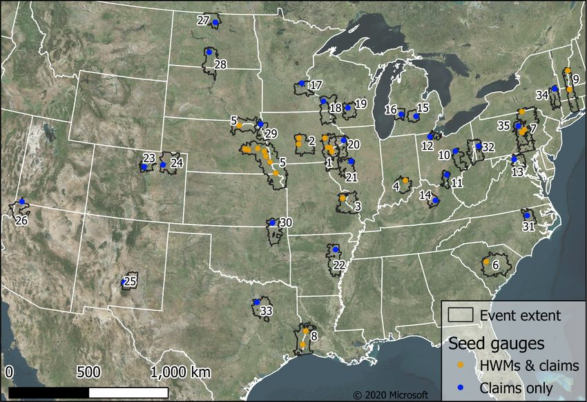
560                                          O. E. J. Wing et al.: Simulating historical flood events at the continental scale

2018; Sampson et al., 2015; Wing et al., 2017; Winsemius          events at most – indeed, a single test case is typical (e.g. Hall
et al., 2013; Yamazaki et al., 2011). These models sacrifice      et al., 2005; Hunter et al., 2008; Mason et al., 2003; Mat-
some local accuracy compared to the traditional engineer-         gen et al., 2007; Neal et al., 2009; Pappenberger et al., 2006;
ing approach but benefit from complete spatial coverage and       Schumann et al., 2011; Stephens et al., 2012; Wood et al.,
the ability to be re-run as climatic and landscape conditions     2016). An analysis of simulation performance across a wider
change, all within reasonable timescale and resource limits.      variety of temporal and spatial settings would provide a
One question that remains to be answered in this field of en-     more reliable evidence case of model validity. To practicably
quiry regards how much local accuracy is lost.                    achieve this, it is necessary to replace the onerous manual
   To answer it, these large-scale inundation models must         construction and parameterisation of local-scale models with
be validated, but two critical barriers prevent this from tak-    a consistent regional- to global-scale model-building frame-
ing place routinely and rigorously. Firstly, design flood maps    work capable of deployment for any model domain within its
of this nature do not represent something observable in re-       realm.
ality. The 100-year flood, for instance, is not a tangible           Furthermore, the replication of historical flood events has
phenomenon, since real flood events do not have spatially         value beyond scientific validation. While design flood maps
static return periods. In producing something theoretical, it     are useful for skilled practitioners who (mostly) understand
is impossible to validate it against something real. Model-       what the models purport to represent, the maps can seem ab-
to-model comparisons – where one model is deemed to be            stract and unconvincing to members of the public since they
suitably accurate so as to be the benchmark, while the other      simulate something intangible and theoretical; thus, knowl-
is the one to be tested – are therefore necessitated. The sec-    edge of the statistical meaning and uncertain derivation of a
ond barrier, then, is the low availability of suitable model      design flood is required to correctly comprehend them (Bell
benchmarks. Global flood models have been compared to lo-         and Tobin, 2007; Luke et al., 2018; Sanders et al., 2020).
cal engineering flood maps in Europe and the US but only          Producing flood maps of historical events – providing an ex-
for a small handful of river basins, inhibiting wide-area test-   plicit understanding of where has flooded in the past – can
ing (Dottori et al., 2016; Sampson et al., 2015; Ward et          aid in motivating private mitigation efforts where the risk
al., 2017; Winsemius et al., 2016). Wing et al. (2017) pre-       perception formed via a design flood map often fails to do
sented a model of the contiguous US, adopting the higher-         so (Bubeck et al., 2012; Kousky, 2017; Luke et al., 2018;
quality hydrographic, hydrometric, terrain, and protection        Poussin et al., 2014). As such, en masse replication of his-
data available in the US compared to available data globally.     torical flood events at high resolution may have value in en-
They compared their model to FEMA’s large, yet incomplete,        hancing risk awareness and the willingness of individuals to
database of 100-year flood maps, charting a high degree of        take mitigatory action.
similarity between the large-scale model and the engineering         In this paper, we adapt the existing continental-scale de-
approach espoused by FEMA. Wing et al. (2019) furthered           sign flood model framework of Bates et al. (2020) to repli-
this examination with statewide engineering models from the       cate historical flood events across the contiguous US. Flood
Iowa Flood Center, coming to similar conclusions. While           events are isolated from US Geological Survey (USGS)
these studies provide useful indications of large-scale model     river gauge data, which form inflow boundary conditions
accuracy, they are fundamentally limited in their characteri-     to a ∼ 30 m resolution 2D hydrodynamic model. High wa-
sation of skill through model intercomparisons. The bench-        ter mark surveys from the USGS were sourced for nine of
mark data in these analyses may share many of the same bi-        the simulated events which, alongside derived flood extents,
ases (e.g. friction parameterisation, channel schematisation,     were used to validate the model. Insurance and assistance
structural error, terrain data precision, and boundary condi-     claims were obtained for 35 flood events to further anal-
tion characterisation) as the model being tested and so not       yse the model’s skill in the context of exposure. By vali-
usefully describe the extent to which it is behavioural.          dating against an order of magnitude greater number of his-
   Model validation, rather than model intercomparison, can       torical flood event observations that exist in academic liter-
only be executed through benchmarking against observa-            ature to date, the analysis provides robust evidence of large-
tions. To do so, the hydraulic models must replicate real-        scale model skill for the first time. To aid in enhancing risk
world events rather than frequency-based flood maps. This         awareness amongst the US public, these flood event foot-
would, by proxy, enable typical applications of design flood      prints have been released on https://floodfactor.com/ (last ac-
maps (such as planning or regulatory decisions, insurance         cess: 3 February 2021), which is a free and accessible tool for
pricing, or emergency response) generated by such a model         Americans to understand their flood risk. Section 2 describes
to be carried out with a richer understanding of its biases.      the methods behind the event replication model and the val-
This is common practice in event-replicating, local-scale,        idation procedures undertaken. In Sect. 3, the results of the
engineering-grade inundation modelling studies. However,          model validation are presented and discussed. Conclusions
their limited spatial scale, laborious manual set-up, and the     are drawn in Sect. 4.
scarce availability of validation data result in observational
benchmarking against only a handful of real-world flood

Nat. Hazards Earth Syst. Sci., 21, 559–575, 2021                                   https://doi.org/10.5194/nhess-21-559-2021
O. E. J. Wing et al.: Simulating historical flood events at the continental scale                                           561

2     Methods                                                     (Bates et al., 2010). River flows are routed through channels
                                                                  defined by the USGS National Hydrography Dataset. Chan-
2.1    USGS gauge input and event selection                       nels are retained as 1D sub-grid features, permitting river
                                                                  widths narrower than the grid resolution (Neal et al., 2012).
USGS river gauge data were initially filtered into those rep-     Channel bathymetry is estimated based on the assumption
resenting catchments which have an upstream area of >             that they can convey the 2-year discharge, which is based on
10 000 km2 and a record length of > 50 years. Of these, one       the Smith et al. (2015) regionalised flood frequency analy-
gauge was selected for each level eight USGS Hydrologic           sis (RFFA) but using USGS river gauges (Bates et al., 2020).
Unit (i.e. HUC8), and the largest event in the record was ex-     Ungauged river channels within each model domain prop-
tracted. This filtering ensured that large loss-driving events,   agated the RFFA-derived mean annual flow instead. Flood
for which validation data were more likely to be available and    protection measures are implemented directly into the model,
whose return periods could be more robustly estimated, were       using a database of adaptations compiled from the US Army
captured. This yielded roughly 200 river gauge events, 50 of      Corps of Engineers National Levee Database and hundreds
which had suitable validation data (see Sect. 2.3). Model do-     of other sub-national databases. For further information, in-
mains of a 50 × 50 km area were constructed around these          cluding details on the aforementioned model-to-model vali-
50 seed gauges, and within each domain, all USGS river            dation, the reader is referred to Wing et al. (2017) and Bates
gauges within it were selected (regardless of drainage area       et al. (2020).
or record length) to ensure all gauged event flows were cap-
tured. Hydrographs spanning 7 d were then extracted from          2.3   Event validation
each gauge for each event, with the seed gauge peak at its
temporal centre. To account for the uncertainty due to stage      High water marks (HWMs) were obtained for nine of the
measurement error and rating curve configuration in the gen-      simulated events from the USGS Flood Event Viewer (https:
eration of the gauged discharges (Coxon et al., 2015; Di Bal-     //stn.wim.usgs.gov/FEV/, last access: 3 February 2021).
dassarre and Montanari, 2009; McMillan et al., 2012), we          HWMs were filtered based on (i) the presence of a nearby up-
simulate each event three times, i.e. the reported discharges     stream river gauge, which ensured the model was only tested
and ±20 %, producing a 0.8*Q, 1.0*Q, and 1.2*Q model              on floodplains it simulated, (ii) a designation of being high
for each event. Some of these 50 gauge events were from           quality, and (iii) the North American Vertical Datum of 1988
the same (particularly widespread) flood event. Once si-          (NAVD 88) being the vertical datum of the reference, consis-
multaneous events were merged post-simulation, 35 discrete        tent with the model terrain data. The number of HWMs re-
flood events remained. Figure 1 illustrates the location of the   tained for each event is shown in Table A1. The surveyed wa-
events, with additional information provided in Table A1.         ter surface elevation (WSE) from each flood event was com-
                                                                  pared to that of the nearest inundated pixel of the modelled
2.2    Hydraulic model                                            maximum inundation extent. Performance was summarised
                                                                  using the following simple equations:
The USGS river flows form the input to the First Street Foun-               N
dation National Flood Model (FSF-NFM) built in collabora-
                                                                            P
                                                                                |WSEmod − WSEobs |
tion with Fathom. The model was first presented by Wing           Error =
                                                                            1
                                                                                                     ,                       (1)
et al. (2017), with updates specified in Bates et al. (2020),                          N
based on the original global modelling framework of Samp-                   N
                                                                            P
son et al. (2015). Terrain data are based on the USGS Na-                       (WSEmod − WSEobs )
                                                                            1
tional Elevation Dataset (NED), with hydraulic simulations        Bias =                             ,                       (2)
                                                                                      N
run at the native resolution of 1 arcsec (∼ 30 m). Other lo-
cal sources of more accurate terrain data were also compiled      where N is the number of HWMs, and the subscripts “mod”
into the data set where available, with ∼ 30 m water surfaces     and “obs” represent modelled and observed WSEs, respec-
downscaled to ∼ 3 m in locations where such fine-resolution       tively. Error indicates the absolute deviation of the modelled
data are present. Gesch et al. (2014) report relative vertical    WSE from the observed WSE, i.e. on average, what is the
errors (point-to-point accuracy; measuring random errors ex-      magnitude of model prediction error? This is commonly re-
clusive of systematic errors), which is more relevant control     ferred to as the mean absolute error (MAE), which is less sen-
on inland flood inundation modelling accuracy than abso-          sitive to outliers than the root mean squared error (RMSE).
lute vertical errors, in the NED of 1.19 m. Most, but not all,    Bias illustrates whether the modelled WSEs are generally
events were located in areas where the NED consists of li-        higher or lower than the observed WSE, i.e. on average, does
dar, with an associated point-to-point accuracy of ∼ 0.66 m       the model over or underpredict WSEs?
(Gesch et al., 2014). The computational hydraulic engine is          To examine model skill in the context of flood extent pre-
based on LISFLOOD-FP, which solves a local inertial for-          diction, HWMs are converted to maps of flood inundation,
mulation of the shallow water equations in two dimensions         in line with the methods of Watson et al. (2018). Firstly, the

https://doi.org/10.5194/nhess-21-559-2021                                   Nat. Hazards Earth Syst. Sci., 21, 559–575, 2021
562 O. E. J. Wing et al.: Simulating historical flood events at the continental scale
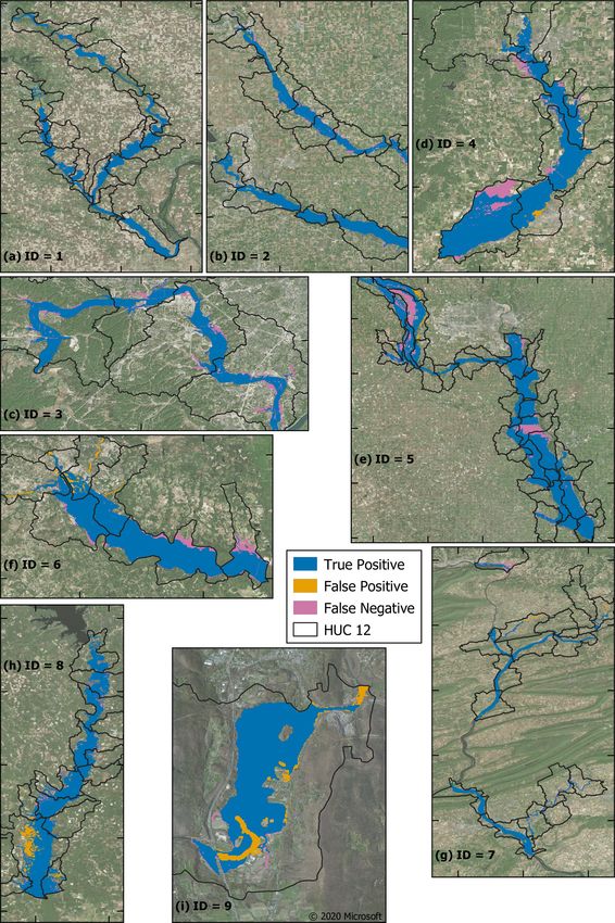
Figure 1. Geographic distribution of 35 simulated events across the contiguous US. Coloured points represent the seed gauges and the
available validation data; black outlines show the discrete event boundaries and associated IDs.
HWMs are interpolated to produce a 2D surface of WSEs claims data sets for the year of the simulated event. The to-
across the model domain. These are then subtracted from ter- tal number of claims (IA and NFIP) were then computed for
rain data, resulting in a grid of water depths. Values greater each of those zip codes. Meanwhile, the number of building
than 0 m therefore fall within the flood extent. Areas of flood- centroids inundated was computed for each zip code using
ing disconnected from the river channel are removed. To pre- Microsoft Building Footprint data. Simple statistical sum-
vent the generation of flood extents in areas for which there maries of the errors are reported, including the coefficient
are no relevant HWMs, inundation maps are only produced of determination (R 2 ) as follows:
in river basins (based on level 12 USGS Hydrologic Units)
N
which contain at least one HWM. These observation-based
(Cobs − Cmod )2
P
flood extents are then compared with the extents simulated 1
by the model, using the critical success index (CSI) described R2 = 1 − , (4)
N
P 2
below: Cobs − Cobs
1
M1 O1
CSI = , (3)
M1 O1 + M1 O0 + M0 O1 where C is the count of inundated buildings observed (obs )
in OpenFEMA data or simulated by the model (mod ) across
where M and O refer to modelled and observed pixels, re-
N = 35 events. This metric, bounded between −∞ and 1, in-
spectively, and the subscripts 1 and 0 indicate whether these
dicates the predictive capabilities of the model through com-
pixels are wet or dry, respectively. This metric divides the
paring the residual variance with the data variance. A perfect
number of correctly wet pixels by the number of pixels which
model would obtain an R 2 of 1, while (subjectively) accept-
are wet in either the modelled or observed data. This general
able models would obtain R 2 > 0.5.
fit score, falling between 0 and 1, accounts for both over- and
under-prediction errors.
Beyond purely flood-hazard-based validation, we sourced 3 Results and discussion
counts of buildings which were inundated during the sim-
ulated events. Individual Assistance (IA) and National 3.1 Water surface elevation comparison
Flood Insurance Program (NFIP) claims data were gath-
ered from the OpenFEMA database (https://www.fema. The results of the HWM validation are shown in Table 1 and
gov/about/reports-and-data/openfema, last access: 3 Febru- visualised in Fig. 2. Biases (Eq. 2) consistently indicate a ten-
ary 2021). For each event, the zip codes that intersected dency towards underprediction for most events, even when
the event inundation layer were selected, and the IA and simulated using 120 % of the gauged discharge. Taking the
NFIP claims data for those zip codes were extracted from the least biased of each event’s three simulations, the mean bias
Nat. Hazards Earth Syst. Sci., 21, 559–575, 2021 https://doi.org/10.5194/nhess-21-559-2021O. E. J. Wing et al.: Simulating historical flood events at the continental scale 563
Figure 2. Box plots of water surface elevation errors for each of the nine simulations. The 25th and 75th percentiles bound the shaded boxes
with medians within. Whiskers are set to a maximum length of 1.5 times the interquartile range beyond the upper or lower quartiles, with
outliers shown as black dots. Box shading refers to the following model discharge input: 80 % (violet), 100 % (green), and 120 % (orange)
of the gauged discharge.
comes to −0.17 m, ranging from −2.95 m for event 3 in Mis- Table 1. Results of the benchmarking of nine events against sur-
souri (2015) to 0.89 m for event 6 in South Carolina (2015) veyed high water marks.
– including a simulation of event 4 in Indiana (2008), with
−0.08 m. Computing errors in line with Eq. (1), which av- ID Bias (m) Error (m)
erages the absolute deviation from the observed water sur- 0.8*Q 1.0*Q 1.2*Q 0.8*Q 1.0*Q 1.2*Q
face elevation, the most accurate of each event’s simulations
1 −0.87 −0.55 −0.17 1.31 1.13 0.96
ranges from 0.31 m (event 4) to 2.95 m (event 3), with a mean 2 −0.61 −0.39 −0.10 0.71 0.53 0.39
of 0.96 m. Most of the events obtain errors in line with the rel- 3 −4.27 −3.75 −2.95 4.27 3.75 2.95
ative vertical accuracy of the NED, which is accurate to be- 4 −0.65 −0.42 −0.08 0.65 0.45 0.31
tween 0.66 and 1.19 m, depending on the terrain data source 5 −1.53 −1.11 −0.70 1.53 1.12 0.74
(Gesch et al., 2014). 6 0.89 1.44 2.07 1.50 1.84 2.35
Surveyed water marks are an excellent tool for validat- 7 −1.31 −0.94 −0.60 1.96 1.85 1.85
8 −1.28 −0.93 −0.59 1.28 0.97 0.66
ing inundation models, though they are not themselves error- 9 0.29 1.05 1.58 1.08 1.22 1.70
free. Numerous past studies sought to quantify uncertainties
in these observational data, finding average vertical errors in Mean −0.17 0.96
the region of 0.3–0.5 m, though, in some cases, these can be
much higher and systematically more biased for particular
https://doi.org/10.5194/nhess-21-559-2021 Nat. Hazards Earth Syst. Sci., 21, 559–575, 2021564 O. E. J. Wing et al.: Simulating historical flood events at the continental scale
sites (Fewtrell et al., 2011; Horritt et al., 2010; Neal et al., Table 2. Results of the benchmarking of nine events against HWM-
2009; Schumann et al., 2007). Given these constraints, typ- derived flood extents.
ical reach-scale hydrodynamic models of inundation events
are calibrated to < 0.4 m deviation from observations of wa- ID Critical success index
ter surface elevation (Adams et al., 2018; Apel et al., 2009; 0.8*Q 1.0*Q 1.2*Q
Bermúdez et al., 2017; Fleischmann et al., 2019; Matgen et
1 0.90 0.92 0.94
al., 2007; Mignot et al., 2006; Pappenberger et al., 2006;
2 0.84 0.88 0.91
Stephens and Bates, 2015; Rudorff et al., 2014). Commonly, 3 0.59 0.70 0.82
the calibration of such models is executed via maximising 4 0.78 0.82 0.86
some measure of fit to the benchmark data by varying the 5 0.73 0.80 0.85
friction parameters (e.g. Pappenberger et al., 2005). Equally, 6 0.85 0.86 0.87
studies have calibrated models by varying other uncertain 7 0.81 0.82 0.83
model features, including channel geometry (e.g. Schumann 8 0.81 0.85 0.88
et al., 2013), terrain data (e.g. Hawker et al., 2018), model 9 0.59 0.88 0.85
structure (e.g. Neal et al., 2011), or boundary conditions Mean 0.87
(e.g. Bermúdez et al., 2017). The model in this study is es-
sentially calibrated by varying the uncertain boundary condi-
tions – though with a sparser exploration of parameter space
(i.e. only three simulations per event) than is typical – to with the bed and water slope roughly parallel (Dottori et al.,
within similar errors found in the literature for some events, 2009). A steady flow profile consistent with the observed
though most events have significantly higher errors. The im- peaks may therefore be more appropriate than linear inter-
pact of discharge uncertainty is evident in the errors of each polation. Given the complexity of fitting a 1D steady flow
simulation per event. Assuming ±20 % error in the observa- model to widespread flood observations, we do not simulate
tion of flood peak stage and its translation to discharge (a it for the purposes of this discussion. Furthermore, incon-
modest assessment of their uncertainties), hydraulic model sistencies in the HWM-derived water surface may often be
errors can increase by between 6 % and 107 % (median of a question of scale, where highly granular topographic fea-
57 %). While this illustrates considerable sensitivity, differ- tures cause a local change in water surface that is inconsistent
ent input discharge configurations within these uncertainty with the reach-scale water levels. Notwithstanding the diffi-
bounds failed to induce an inundation model replication of culties in understanding water surfaces across a river reach
the HWM elevations for most events. with relatively sparse 1D observations, these comparisons do
To further contextualise the results obtained here, we anal- lead one to question whether the water slopes purported by
yse the hydraulic plausibility of the surveyed HWMs along the HWMs in Fig. 3 are physically realistic. When the data
selected river reaches. Figure 3a shows the profile of the points in Fig. 3 are restricted to within 1 km of gauge loca-
water surface elevation experienced during the 2008 event tions, the HWMs deviate from the interpolated surface by
on the Cedar River. Figure 3c shows the same but for the 0.79 m (Cedar River) and 0.94 m (Platte River) on average.
Platte River event in 2019. It is clear that the HWMs pro- These observational data, then, may have higher errors than
duce some local water surfaces which qualitatively appear similar data reported in the wider literature, which provides
inconsistent and implausible at the reach scale. No hydraulic a useful context for the 0.96 m mean error obtained by the
model obeying mass and momentum conservation laws could model here.
feasibly reproduce such water surfaces. For these events, lo-
cal USGS river gauges are obtained (Cedar River – 05453520 3.2 Flood extent comparison
and 05464000; Platte River – 06796000, 06801000, and
06805500), and a water surface for the considered reaches When examining the differences between the simulated max-
is linearly interpolated between these. While being an unreli- imum flood extents and those produced from interpolating
able estimate of WSE far from gauged locations, this interpo- the HWMs over relevant river basins in the terrain data, the
lated surface provides a useful indicator of how HWM WSEs model obtains a CSI of 0.87 on average (see Table 2). Event 3
vary across the river reaches (see Fig. 3b and d). Altenau et in Missouri obtains the lowest maximum CSI of 0.82, while
al. (2017a) measured water surface elevations at ∼ 100 m in- the highest, of 0.94, is held by event 1 in Iowa. Optimum
tervals along a 90 km reach of the Tanana River, AK, using simulations and their comparison to the observation-based
airborne radar. The radar data, shown to be highly accurate extents are shown in Fig. 4.
(±0.1 m) when compared to field measurements, illustrated Typical reach-scale 2D inundation models generally ob-
a smooth and approximately linear slope, even for a com- tain CSIs of 0.7–0.8 when calibrated to air- or space-borne
plex, braided river. However, this campaign did not take place imagery of flood extents (Aronica et al., 2002; Di Baldas-
during a flood event. Bed slopes akin to those on the Platte sarre et al., 2009; Horritt and Bates, 2002; Pappenberger et
River suggest that the flood wave would be quasi-kinematic, al., 2007; Stephens and Bates, 2015; Wood et al., 2016).
Nat. Hazards Earth Syst. Sci., 21, 559–575, 2021 https://doi.org/10.5194/nhess-21-559-2021O. E. J. Wing et al.: Simulating historical flood events at the continental scale 565 Figure 3. Water surface profiles based on gauge and high water mark data for (a, b) the Cedar River between Cedar Falls and Waterloo, Iowa (event 1), and (c, d) the Platte River near Omaha, Nebraska (event 5). Profiles in (a) and (c) are referenced to mean sea level, while those in (b) and (d) adopt the interpolated gauged water surface as the vertical datum. Where observations and their classification methods are of for each of the nine events is compared. While a generally high quality, CSIs of up to 0.9 can be obtained (Altenau et al., intuitive negative relationship between CSI and water level 2017b; Bermúdez et al., 2017; Bates et al., 2006; Stephens et error is exhibited (Pearson’s r = −0.6), CSIs do not drasti- al., 2012). The model here obtained CSIs of 0.8–0.9 when cally reduce as water level errors increase. The reasons for benchmarked against interpolated HWMs rather than actual this seeming CSI insensitivity relate to specific characteris- 2D observations of flood extent. Where HWMs are sparsely tics of each event. Events on the Congaree and Connecticut spaced, the interpolated flood extent may not have accurately rivers (events 6 and 9) have fairly large water level errors replicated the true flood extent. Thus, while it is likely that in spite of excellent CSIs. This is because, in both modelled the model has replicated the uncertain benchmark flood ex- and observed floods, the floodplain was filled up, meaning tents to within error, setting a precedent for CSIs in the wider that extent comparisons were less sensitive to model over- literature can often provide misinformation. In Fig. 5, the re- prediction. These events were simulated with an overpredic- lationship between minimum WSE error and maximum CSI tion bias, i.e. there was too much water on the floodplain (in https://doi.org/10.5194/nhess-21-559-2021 Nat. Hazards Earth Syst. Sci., 21, 559–575, 2021
566                                          O. E. J. Wing et al.: Simulating historical flood events at the continental scale

Figure 4. Maps illustrating the similarity between modelled flood events and HWM-derived extents in relevant hydrologic unit code
(HUC) 12 zones. Interior tick marks are spaced 0.25◦ (∼ 27 km) apart. Imagery sourced from © 2020 Microsoft.

three dimensions), but this made little difference to flood ex-    Even the event on Meramec River (event 3) obtained a CSI il-
tent (in two dimensions). In contrast, the event on Flatrock       lustrative of high performance, despite very high water level
River (event 4), which is characterised by low WSE errors,         errors. This particular flood was large in magnitude, mean-
obtained a comparable CSI to events 6 and 9. While verti-          ing that the reward for capturing the numerous inundated ar-
cal errors were small, the model did not completely repli-         eas overshadowed the penalisation for underestimating the
cate the larger flood inundation across the low-gradient ter-      flood edge. In the vertical plane, however, the Meramec River
rain represented by the benchmark flood extent for event 4.        event simulation is shown to significantly underpredict wa-

Nat. Hazards Earth Syst. Sci., 21, 559–575, 2021                                   https://doi.org/10.5194/nhess-21-559-2021
O. E. J. Wing et al.: Simulating historical flood events at the continental scale                                                  567

Figure 5. The relationship between the WSE error and flood extent CSI for the nine events. Numbered crosses refer to the ID of the flood
event.

ter surface elevation. Meanwhile, the model was rightly re-           meaning ungauged tributaries and other lateral inflows within
warded by both metrics for correctly simulating the Iowa              the model domain were not properly accounted for. In fail-
2008 floods (events 1 and 2) – large floods on large rivers –         ing to simulate the aggregation of these flows, the volume of
by filling up the floodplains with reasonably low water level         water within and exiting the model was likely much lower
errors. These examinations build on the evidence provided by          than reality for many of the flood events, resulting in a corre-
Stephens et al. (2014), who noted that similar water level er-        spondingly underpredicting inundation model.
rors can result in different CSIs, depending on the size of the
flood, the valley gradient, and the sign of model bias. Mason         3.3   Inundated building comparison
et al. (2007, 2009) similarly posit that an analysis of water
height offers a way of discriminating between the equifinal           The results after using FEMA claims data to validate the full
model structures that extent comparisons tend to result in.           set of 35 events are shown in Fig. 6. Only nine events sim-
For this analysis of a larger sample of flood events, we reaf-        ulate the correct number of claims within the discharge un-
firm their conclusions that CSIs cannot be easily compared            certainty bounds. When considering the closest match simu-
for events of different natures, and that a comparison against        lation (of the three) in terms of inundated buildings for each
water levels is a more discriminatory metric.                         event, the mean error in the simulated counts of building in-
   The extremely large underprediction errors for the Mer-            undation is 26 % of the observed count. The standard devia-
amec River flood event simulation (event 3) may be ex-                tion of this quantity is 132 %, reflecting the substantial scatter
plained by its nature as a tributary of the Mississippi River         evident in Fig. 6. The modelled building inundation obtains
and the arbitrary nature of the geographic domains that the           an R 2 (Eq. 4) of 0.63. In general, it appears that more catas-
automated model builder produces. Even adding 20 % to the             trophic events (in terms of inundated buildings) are more fre-
reported USGS discharges resulted in an underprediction of            quently underpredicted by the model, i.e. nine events under-
water surface elevations by roughly 3 m. It is likely that this       predict building inundation compared to three which over-
flood event was primarily driven by Meramec River flows               predict for events with > 500 inundated buildings. Mean-
backing up against the Mississippi River. With no Missis-             while, less catastrophic events are seemingly systematically
sippi River gauge within the 50 km radius of the Meramec              overestimated, i.e. 10 events overpredict and four events un-
River seed gauge, the Mississippi River was not also in flood         derpredict for events with < 500 inundated buildings. This
during the simulation. In the absence of a correct downstream         is perhaps explained by the nature of the validation data. The
boundary inducing a backwatering effect, the Meramec River            sum of NFIP and IA claims may not account for all inundated
flood flowed freely down the Mississippi River in the simula-         buildings during an event. Impacted households may obtain
tion rather than onto the Meramec River floodplain. The gen-          assistance from local governments (with or without aid from
eral underprediction bias across most flood events is likely          the federal Public Assistance programme), low-interest dis-
explained by river gauge density. Boundary conditions are             aster loans from the Small Business Administration, have
only available in the presence of a USGS gauging station,             private insurance, or simply require no external aid – none
                                                                      of which are captured by the sum of NFIP and IA claims.

https://doi.org/10.5194/nhess-21-559-2021                                       Nat. Hazards Earth Syst. Sci., 21, 559–575, 2021
568 O. E. J. Wing et al.: Simulating historical flood events at the continental scale The validation data in this instance are almost certainly un- derestimates of the true count of affected buildings; the mag- nitude of this underestimation is unknown, though is likely non-negligible. A total of 10 of the 18 events with < 500 ob- served inundated buildings consist entirely of NFIP claims, while only one of the 17 events with > 500 observed in- undated buildings share this characteristic. This is because IA can only be claimed when the associated event is declared as a disaster by the president. Typically, these are larger dis- asters which exceed the state or local government’s capacity to respond. As such, uninsured (via the NFIP) households impacted by these smaller events (in a risk context) who are unable to claim IA will be uncounted in this analysis, as they likely received assistance from other sources. Hence, the overprediction bias for these less catastrophic events ap- pears intuitive. Potential causes of the underprediction biases in Fig. 6 have been highlighted previously in this section. Difficulties in defining a downstream boundary may have in- duced a more confined flood to be modelled than reality, and low river gauge density may have resulted in some damage- causing tributary floods to remain unmodelled. As for some of the more extreme cases of underprediction, such as the flood events in South Carolina (event 6; ∼ 10 000 observed versus ∼ 1000 modelled inundated buildings) and Kansas (event 30; ∼ 2000 observed versus ∼ 400 modelled inun- dated buildings), these may be explained by much of the risk being pluvial driven. Since the rainfall component of the Bates et al. (2020) model was not utilised here, urban, rainfall-driven, flash flooding – which contributed to many of the inundated buildings for these events – was not captured. Furthermore, in Fig. 7 we can see that the model skill pur- ported by the inundated building analysis bears little relation to the flood elevation and extent errors for the nine events with this information. A positive relationship would be ex- pected in Fig. 7a, while a negative relationship would be expected in Fig. 7b. Event 7 in Pennsylvania is one of the least skilful events in the hazard-based analysis (WSE error of 1.85 m; CSI of 0.83), yet it is within discharge error of the observed inundated building count. Of course, the inun- dated building analysis does not measure whether the correct Figure 6. Scatter plots illustrating the observed (NFIP and IA) buildings are inundated. Instead, it tests whether the same versus the modelled count of inundated buildings for each of the number of buildings are inundated in aggregate, which could 35 events. Blue crosses represent the simulated count in the 1.0*Q be a fortuitous balance of type I and II errors. In spite of model, with error bars representing the range of counts between this, and incorporating Fig. 5 into this discussion, it is clear the 0.8*Q and 1.2*Q simulations. The trend line represents a linear that the choice of model test and the spatio-temporal set- polynomial fitted to the optimum of each event’s three simulations. ting of the test holds enormous sway over how one interprets Descending panels are sequentially more magnified towards the ori- the model’s efficacy. High water level errors may have little gin. impact on a model’s ability to replicate impacted buildings; equally, inundated building counts may be highly sensitive to small water level errors. Coupled with the inconsistency interrogate the model’s skill are layered on top of this, for in skill scores – of any metric – between flood events of dif- instance: (i) errors against HWMs are often high, but, from ferent magnitudes, locations, data richness, and other char- Fig. 3, we can see that these field data sometimes make lit- acteristics, it makes obtaining an objective and generalised tle hydraulic sense, containing errors themselves perhaps ap- assessment of the US flood model employed here challeng- proaching those obtained by the model in many instances; ing. The likely considerable uncertainties in the data used to (ii) the resultant extents derived from these will share their Nat. Hazards Earth Syst. Sci., 21, 559–575, 2021 https://doi.org/10.5194/nhess-21-559-2021
O. E. J. Wing et al.: Simulating historical flood events at the continental scale                                                     569

Figure 7. The relationship between inundated building count errors and (a) WSE error and (b) flood extent CSI for the nine events. Numbered
crosses refer to the ID of the flood event.

biases and, particularly in areas unconstrained by HWMs,                tests of flood extent similarity can mask large deviations be-
the interpolated surface may not represent reality well; and            tween observed and simulated water surface elevation. While
(iii) no reliable and integrated data exist on exact counts of          all events were well replicated in terms of flood extent, water
buildings impacted by flood events, meaning the assimila-               surface elevation errors were roughly 1 m on average. Some
tion of NFIP and IA claims used here likely underpredict the            events adequately replicated the WSEs recorded in the HWM
true value of this quantity. Whether a model is deemed good             data, while others were considerably underestimated. How-
therefore depends on what it is simulating and for what pur-            ever, most event water level errors are within the relative ver-
pose, in addition to considering the influence of an unknown            tical errors of the terrain data employed. The impact of plau-
upper limit on the desired closeness of the match between the           sible (and perhaps conservative) errors in the high flow mea-
model and uncertain validation data.                                    surements used to drive the model is shown to affect its skill
                                                                        substantially, yet it is also clear that other errors remain. The
                                                                        insensitivity of extent comparison scores to changing water
4   Conclusions                                                         level errors suggests that CSIs are not readily comparable
                                                                        for different types of flood events; a model obtaining a CSI
In this analysis, we devised a framework to construct and de-           of 0.8 for event A may be no more skilful (in terms of water
ploy hydrodynamic models for any recorded historical flood              level error) than one which obtains a CSI of 0.6 for event B.
event in the US, with minimal manual intervention, using                We reiterate here the conclusions from other bodies of work
the continental-scale design flood model described by Bates             (e.g. Mason et al., 2009; Stephens et al., 2014) which suggest
et al. (2020). We obtained hydrologic field observations for            that an analysis of water surface elevations provides a more
nine events simulated by this framework and recordings of               rigorous and discriminatory test of a flood inundation model.
inundated buildings for 35 such events in order to examine              In the analysis of buildings inundated by the larger set of
the skill of the model. Not unexpectedly, we find that model            flood events, some perfectly replicated the observed count of
skill varies considerably between events, suggesting that the           buildings while others starkly deviated from this. The 26 %
testing of flood inundation models across a spatial-scale im-           mean error and an R 2 of 0.63 still indicates reasonably strong
balance (i.e. benchmarking continental–global-scale models              predictive skill of these quantities by the model.
against a handful of localised test cases) is prone to a mis-              A consideration of the error in the observational valida-
leading evaluation of its usefulness. Previous studies sug-             tion data is often overlooked when interpreting the efficacy
gest that the continental model employed here can replicate             of a flood inundation model. If the deviation between the true
the extent of high-quality, local-scale models of large flood           maximum water surface elevation achieved during a flood
events within error (Wing et al., 2017, 2019; Bates et al.,             event and that recorded from a high water mark is upwards
2020). Similarly, this analysis illustrates the very close match        of 0.5 m, obtaining model-to-observation errors of less than
between flood extents derived from field data collected dur-            0.5 m would be the result of rewarding the replication of
ing the flood events and the maximum flood extent simulated             noise. In this analysis, the magnitude of observational uncer-
by the continental model. However, we also highlight that

https://doi.org/10.5194/nhess-21-559-2021                                         Nat. Hazards Earth Syst. Sci., 21, 559–575, 2021
570 O. E. J. Wing et al.: Simulating historical flood events at the continental scale
tainties is not formally examined, yet for many of the tests,
the value of the validation data was close to exhaustion, i.e.
a given benchmark was often replicated within its likely er-
ror. The HWMs did not always produce consistent water sur-
faces, interpolating between these may produce unrealistic
flood extents at some locations, and the source of inundated
building data may have undercounted the true number of im-
pacted households.
In spite of this, useful interpretations of model perfor-
mance can still be drawn from this analysis. The automated
large-scale model is capable of skilfully replicating histori-
cal flood events, though, in some circumstances, events are
poorly replicated and are generally so with an underpredic-
tion bias. This can be addressed by further developments to
the event replication framework, which include the addition
of a pluvial model component and restricting event domains
to those which contain downstream (and not just upstream)
river gauges to better represent backwatering. Furthermore,
the use of hydrological models would solve the issue of
gauge density and would also enable an estimation of future
inundation hazards, which this framework cannot presently
execute. However, the additional error induced by employing
simulated, rather than observed, discharges would need to be
considered. While these will be explored in future research,
it is also clear from this analysis that flood inundation models
can rarely be comprehensively validated when using histori-
cal data. Routinely collected terrain, boundary condition, and
validation data must improve drastically for the science in
this field to advance meaningfully. To do this, dedicated and
specialist field campaigns are required, though it should be
recognised that mobilising such a resource in time to capture
transient events safely during extreme floods will be chal-
lenging. To this end, complementary data from remote sens-
ing observations – particularly with the forthcoming launch
of the NASA Surface Water and Ocean Topography (SWOT)
mission – will necessarily play a role.
Nat. Hazards Earth Syst. Sci., 21, 559–575, 2021 https://doi.org/10.5194/nhess-21-559-2021O. E. J. Wing et al.: Simulating historical flood events at the continental scale 571
Appendix A
Table A1. The flood events simulated in this analysis. Return periods were obtained from USGS StreamStats data.
Location Date ID Seed Return Inundated High
gauges period buildings water
(years) marks
Iowa and Cedar rivers, eastern Iowa June 2008 1 4 500 12 108 576
Des Moines and Skunk rivers, central Iowa June/July 2008 2 2 50 3964 166
Meramec River, eastern Missouri December 2015 3 1 100 454 143
Flatrock River, southern Indiana June 2008 4 1 75 3167 298
Missouri and Platte rivers, eastern Nebraska March 2019 5 8 100 5755 1023
Congaree River, central South Carolina October 2015 6 1 20 9768 230
Susquehanna River, northern Pennsylvania September 2011 7 3 150 14 123 273
Sabine River, Texas/Louisiana border March 2016 8 2 1000 5236 22
Connecticut River, New England August 2011 9 2 300 2145 482
Killbuck Creek, eastern Ohio January 2005 10 1 25 393 –
Scioto River, southern Ohio January 2005 11 1 5 351 –
Maumee River, northwestern Ohio June 2015 12 1 25 38 –
Potomac River, Maryland/West Virginia border December 2018 13 1 5 33 –
Kentucky River, central Kentucky May 2004 14 1 25 172 –
Grand River, central Michigan May 2004 15 1 5 192 –
Grand River, western Michigan April 2013 16 1 15 97 –
Mississippi River, eastern Minnesota April 2001 17 1 50 87 –
Mississippi River, southern Minnesota April 2001 18 1 75 113 –
Wisconsin River, central Wisconsin June 2008 19 1 5 871 –
Mississippi River, Iowa/Illinois border April 2001 20 1 100 543 –
Illinois River, central Illinois April 2013 21 1 75 150 –
White River, northern Arkansas May 2011 22 1 25 1231 –
Boulder Creek, northern Colorado September 2012 23 1 1000 3212 –
South Platte River, northeastern Colorado September 2013 24 1 75 349 –
Eagle Creek, southern New Mexico July 2008 25 1 100 50 –
Virgin River, southwestern Utah January 2005 26 1 150 4 –
Souris River, northern North Dakota June 2011 27 1 100 99 –
Missouri River, central North Dakota June 2011 28 1 100 2119 –
Big Sioux River, South Dakota/Iowa border June 2014 29 1 400 33 –
Verdigris River, southeastern Kansas July 2007 30 1 500 2061 –
Tar River, northeastern North Carolina October 2016 31 1 35 323 –
Ohio River, western Pennsylvania September 2004 32 1 10 10 975 –
Trinity River, northeastern Texas May 2015 33 1 50 143 –
Hudson River, eastern New York April 2011 34 1 10 1290 –
Susquehanna River, central Pennsylvania September 2004 35 1 25 1469 –
https://doi.org/10.5194/nhess-21-559-2021 Nat. Hazards Earth Syst. Sci., 21, 559–575, 2021572 O. E. J. Wing et al.: Simulating historical flood events at the continental scale
Data availability. Historical flood events were simulated on be- References
half of the First Street Foundation (https://firststreet.org/, last ac-
cess: 3 February 2021) and form part of their Flood Factor plat- Adams, T. E., Chen, S., and Dymond, R., Results from operational
form (https://floodfactor.com/, last access: 3 February 2021). Hy- hydrologic forecasts using the NOAA/NWS OHRFC Ohio river
drodynamic modelling output is available for non-commercial, aca- community HEC-RAS model, J. Hydrol. Eng., 23, 04018028,
demic research purposes, only upon reasonable request from the https://doi.org/10.1061/(ASCE)HE.1943-5584.0001663, 2018.
corresponding author. USGS terrain data are available from https: Alfieri, L., Salamon, P., Bianchi, A., Neal, J., Bates, P., and
//ned.usgs.gov/ (last access: 3 February 2021) (US Geological Sur- Feyen, L.: Advances in pan-European flood hazard mapping, Hy-
vey, 2021a). USGS river gauge data are available from https:// drol. Process., 28, 4067–4077, https://doi.org/10.1002/hyp.9947,
waterdata.usgs.gov/nwis (last access: 3 February 2021) (US Geo- 2014.
logical Survey, 2021b). USGS high water mark data are available Altenau, E. H., Pavelsky, T. M., Moller, D., Lion, C., Pitcher, L. H.,
from https://stn.wim.usgs.gov/FEV/ (last access: 3 February 2021) Allen, G. H., Bates, P. D., Calmant, S., Durand, M., and Smith,
(US Geological Survey, 2021c). Insurance and assistance claims L. C.: AirSWOT measurements of river water surface elevation
are available from https://www.fema.gov/about/reports-and-data/ and slope: Tanana River, AK, Geophys. Res. Lett., 44, 181–189,
openfema (last access: 3 February 2021) (Federal Emergency https://doi.org/10.1002/2016GL071577, 2017a.
Management Agency, 2021). Microsoft Building Footprints are Altenau, E. H., Pavelsky, T. M., Bates, P. D., and Neal, J. C.:
available from https://github.com/microsoft/USBuildingFootprints The effects of spatial resolution and dimensionality on modeling
(last access: 3 February 2021) (Microsoft, 2021). USGS Stream- regional-scale hydraulics in a multichannel river, Water Resour.
Stats are available from https://streamstats.usgs.gov/ (last access: Res., 53, 1683–1701, https://doi.org/10.1002/2016WR019396,
3 February 2021) (US Geological Survey, 2021d). USGS HUC 2017b.
zones are available from https://water.usgs.gov/GIS/huc.html (last Apel, H., Aronica, G. T., Kreibich, H., and Thieken, A. H., Flood
access: 3 February 2021) (US Geological Survey, 2021e). The risk analyses – how detailed do we need to be?, Nat. Hazards, 49,
United States Army Corps of Engineers (USACE) National Levee 77–98, https://doi.org/10.1007/s11069-008-9277-8, 2009.
Database is available at https://levees.sec.usace.army.mil/ (last ac- Aronica, G., Bates, P. D., and Horritt, M. S.: Assessing the uncer-
cess: 3 February 2021) (US Army Corps of Engineers, 2021). The tainty in distributed model predictions using observed binary pat-
USGS National Hydrography Dataset is available at https://www. tern information within GLUE, Hydrol. Process., 16, 2001–2006,
usgs.gov/core-science-systems/ngp/national-hydrography (last ac- https://doi.org/10.1002/hyp.398, 2002.
cess: 3 February 2021) (US Geological Survey, 2021f). Association of State Floodplain Managers: Flood Mapping for the
Nation: A Cost Analysis for Completing and Maintaining the Na-
tion’s NFIP Flood Map Inventory, Madison, WI, USA, 2020.
Author contributions. OEJW performed the hydraulic analyses of Bates, P. D., Wilson, M. D., Horritt, M. S., Mason, D. C.,
the models and wrote the paper. AMS and CCS developed and ran Holden, N., and Currie, A.: Reach scale floodplain inunda-
the models. MLM performed the analyses relating to the building tion dynamics observed using synthetic aperture radar im-
data. JRP and MFA conceived the project. All authors aided in the agery: data analysis and modelling, J. Hydrol., 328, 306–318,
conceptualisation of the analysis and commented on initial drafts. https://doi.org/10.1016/j.jhydrol.2005.12.028, 2006.
Bates, P. D., Horritt, M. S., and Fewtrell, T. J.: A simple inertial
formulation of the shallow water equations for efficient two-
dimensional flood inundation modelling, J. Hydrol., 387, 33–45,
Competing interests. The authors declare that they have no conflict
https://doi.org/10.1016/j.jhydrol.2010.03.027, 2010.
of interest.
Bates, P. D., Quinn, N., Sampson, C. C., Smith, A. M., Wing,
O. E. J., Sosa, J., Savage, J., Olcese, G., Schumann, G. J.-P.,
Giustarini, L., Coxon, G., Neal, J. C., Porter, J. R., Amodeo,
Acknowledgements. The authors are indebted to the US Geological M. F., Chu, Z., Lewis-Gruss, S., Freeman, N., Houser, T., Del-
Survey for their continued efforts in providing easy and open access gado, M., Hamidi, A., Bolliger, I. W., McCusker, K. E., Emanuel,
to data sets fundamental to the construction and assessment of flood K. A., Ferreira, C. M., Khalid, A., Haigh, I. D., Couasnon, A.,
inundation models in the US. Kopp, R. E., Hsiang, S., and Krajewski, W. F.: Combined mod-
elling of US fluvial, pluvial and coastal flood hazard under cur-
rent and future climates, Water Resour. Res., e2020WR028673,
Financial support. Oliver E. J. Wing and Paul D. Bates were sup- https://doi.org/10.1029/2020WR028673, accepted, 2020.
ported by the Engineering and Physical Sciences Research Council Bell, H. M. and Tobin, G. A.: Efficient and effective?
(EPSRC; grant no. EP/R511663/1). Paul D. Bates was supported by The 100-year flood in the communication and per-
a Royal Society Wolfson Research Merit Award. ception of flood risk, Environ. Hazards, 7, 302–311,
https://doi.org/10.1016/j.envhaz.2007.08.004, 2007.
Bermúdez, M., Neal, J. C., Bates, P. D., Coxon, G., Freer, J. E.,
Review statement. This paper was edited by Philip Ward and re- Cea, L., and Puertas, J., Quantifying local rainfall dynamics
viewed by Marc Bierkens and Francesco Dottori. and uncertain boundary conditions into a nested regional-local
flood modeling system, Water Resour. Res., 53, 2770–2785,
https://doi.org/10.1002/2016WR019903, 2017.
Bubeck, P., Botzen, W. J. W., and Aerts, J. C. J. H.: A
review of risk perceptions and other factors that influ-
Nat. Hazards Earth Syst. Sci., 21, 559–575, 2021 https://doi.org/10.5194/nhess-21-559-2021O. E. J. Wing et al.: Simulating historical flood events at the continental scale 573
ence flood mitigation behavior, Risk Anal., 32, 1481–1495, Horritt, M. S., Bates, P. D., Fewtrell, T. J., Mason, D.
https://doi.org/10.1111/j.1539-6924.2011.01783.x, 2012. C., and Wilson, M. D.: Modelling the hydraulics of the
Coxon, G., Freer, J., Westerberg, I. K., Wagener, T., Woods, R., Carlisle 2005 flood event, Proc. Inst. Civ. Eng., 163, 273–281,
and Smith, P. J.: A novel framework for discharge uncertainty https://doi.org/10.1680/wama.2010.163.6.273, 2010.
quantification applied to 500 UK gauging stations, Water Resour. Hunter, N. M., Bates, P. D., Neelz, S., Pender, G., Villanueva, I.,
Res., 51, 5531–5546, https://doi.org/10.1002/2014WR016532, Wright, N. G., Liang, D., Falconer, R. A., Lin, B., Waller, S.,
2015. Crossley, A. J., and Mason, D. C.: Benchmarking 2D hydraulic
Di Baldassarre, G. and Montanari, A.: Uncertainty in river discharge models for urban flooding, Proc. Inst. Civ. Eng. – Water Manage.,
observations: a quantitative analysis, Hydrol. Earth Syst. Sci., 13, 161, 13–30, https://doi.org/10.1680/wama.2008.161.1.13, 2008.
913–921, https://doi.org/10.5194/hess-13-913-2009, 2009. Kousky, C.: Disasters as learning experiences or disas-
Di Baldassarre, G., Schumann, G., and Bates, P. D.: A tech- ters as policy opportunities? Examining flood insurance
nique for the calibration of hydraulic models using uncertain purchases after hurricanes, Risk Anal., 37, 517–530,
satellite observations of flood extent, J. Hydrol., 367, 276–282, https://doi.org/10.1111/risa.12646, 2017.
https://doi.org/10.1016/j.jhydrol.2009.01.020, 2009. Luke, A., Sanders, B. F., Goodrich, K. A., Feldman, D. L.,
Dottori, F., Martina, M. L. V., and Todini, E.: A dynamic rat- Boudreau, D., Eguiarte, A., Serrano, K., Reyes, A., Schubert, J.
ing curve approach to indirect discharge measurement, Hydrol. E., AghaKouchak, A., Basolo, V., and Matthew, R. A.: Going
Earth Syst. Sci., 13, 847–863, https://doi.org/10.5194/hess-13- beyond the flood insurance rate map: insights from flood haz-
847-2009, 2009. ard map co-production, Nat. Hazards Earth Syst. Sci., 18, 1097–
Dottori, F., Salamon, P., Bianchi, A., Alfieri, L., Hirpa, F. A., 1120, https://doi.org/10.5194/nhess-18-1097-2018, 2018.
and Feyen, L.: Development and evaluation of a framework for Mason, D. C., Cobby, D. M., Horritt, M. S., and Bates, P. D.:
global flood hazard mapping, Adv. Water Resour., 94, 87–102, Floodplain friction parameterization in two-dimensional river
https://doi.org/10.1016/j.advwatres.2016.05.002, 2016. flood models using vegetation heights derived from airborne
Federal Emergency Management Agency: OpenFEMA, available scanning laser altimetry, Hydrol. Process., 17, 1711–1732,
at: https://www.fema.gov/about/reports-and-data/openfema, last https://doi.org/10.1002/hyp.1270, 2003.
access: 3 February 2021. Mason, D. C., Horritt, M. S., Dall’Amico, J. T., Scott,
Fewtrell, T. J., Duncan, A., Sampson, C. C., Neal, J. C., and T. R., and Bates, P. D.: Improving river flood extent
Bates, P. D.: Benchmarking urban flood models of vary- delineation from synthetic aperture radar using airborne
ing complexity and scale using high resolution terrestrial laser altimetry, IEEE T. Geosci. Remote, 45, 3932–3943,
LiDAR data, Phys. Chem. Earth Pt. A/B/C, 36, 281–291, https://doi.org/10.1109/TGRS.2007.901032, 2007.
https://doi.org/10.1016/j.pce.2010.12.011, 2011. Mason, D. C., Bates, P. D., and Dall’Amico, J. T.: Cal-
Fleischmann, A., Paiva, R., and Collischonn, W.: Can re- ibration of uncertain flood inundation models using re-
gional to continental river hydrodynamic models be locally motely sensed water levels, J. Hydrol., 368, 224–236,
relevant? A cross-scale comparison, J. Hydrol., 3, 100027, https://doi.org/10.1016/j.jhydrol.2009.02.034, 2009.
https://doi.org/10.1016/j.hydroa.2019.100027, 2019. Matgen, P., Schumann, G., Hentry, J.-B., Hoffmann, L., and Pfis-
Gesch, D. B., Oimoen, M. J., and Evans, G. A.: Accuracy Assess- ter, L.: Integration of SAR-derived river inundation areas, high-
ment of the US Geological Survey National Elevation Dataset, precision topographic data and a river flow model toward near
and Comparison with Other Large-Area Elevation Datasets real-time flood management, Int. J. Appl. Earth Obs. Geoinf., 9,
– SRTM and ASTER, US Geological Survey Open-File Re- 247–263, https://doi.org/10.1016/j.jag.2006.03.003, 2007.
port 2014-1008, US Geological Survey, Reston, VA, 10 pp., McMillan, H., Krueger, T., and Freer, J.: Benchmarking ob-
https://doi.org/10.3133/ofr20141008, 2014. servational uncertainties for hydrology: rainfall, river dis-
Hall, J. W., Tarantola, S., Bates, P. D., and Horritt, M. S.: Distributed charge and water quality, Hydrol. Process., 26, 4078–4111,
sensitivity analysis of flood inundation model calibration, J. Hy- https://doi.org/10.1002/hyp.9384, 2012.
draul. Eng., 131, 117–126, https://doi.org/10.1061/(ASCE)0733- Microsoft: USBuildingFootprints, available at: https://github.com/
9429(2005)131:2(117), 2005. microsoft/USBuildingFootprints, last access: 3 February 2021.
Hattermann, F. F., Wortmann, M., Liersch, S., Toumi, R., Sparks, Mignot, E., Paquier, A., and Haider, S.: Modeling floods in a dense
N., Genillard, C., Schröter, K., Steinhausen, M., Gyalai- urban area using 2D shallow water equations, J. Hydrol., 327,
Korpos, M., Máté, K., Hayes, B., del Rocío Rivas López, 186–199, https://doi.org/10.1016/j.jhydrol.2005.11.026, 2006.
M., Rácz, T., Nielsen, M. R., Kaspersen, P. S., and Drews, Neal, J., Schumann, G., Fewtrell, T., Budimir, M., Bates, P., and
M.: Simulation of flood hazard and risk in the Danube Mason, D.: Evaluating a new LISFLOOD-FP formulation with
basin with the Future Danube Model, Clim. Serv., 12, 14–26, data from the summer 2007 floods in Tewkesbury, UK, J.
https://doi.org/10.1016/j.cliser.2018.07.001, 2018. Flood Risk Manage., 4, 88–95, https://doi.org/10.1111/j.1753-
Hawker, L., Rougier, J., Neal, J., Bates, P., Archer, L., and Ya- 318X.2011.01093.x, 2011.
mazaki, D.: Implications of simulating global digital elevation Neal, J., Schumann, G., and Bates, P.: A subgrid channel model
models for flood inundation studies, Water Resour. Res., 54, for simulating river hydraulics and floodplain inundation over
7910–7928, https://doi.org/10.1029/2018WR023279, 2018. large and data sparse areas, Water Resour. Res., 48, W11506,
Horritt, M. S. and Bates, P. D.: Evaluation of 1D and 2D numerical https://doi.org/10.1029/2012WR012514, 2012.
models for predicting river flood inundation, J. Hydrol., 268, 87– Neal, J. C., Bates, P. D., Fewtrell, T. J., Hunter, N. M., Wilson, M.
99, https://doi.org/10.1016/S0022-1694(02)00121-X, 2002. D., and Horritt, M. S.: Distributed whole city water level mea-
surements from the Carlisle 2005 urban flood event and compar-
https://doi.org/10.5194/nhess-21-559-2021 Nat. Hazards Earth Syst. Sci., 21, 559–575, 2021You can also read