MEASUREMENT AND MODELLING OF THE DYNAMICS OF NH3 SURFACE-ATMOSPHERE EXCHANGE OVER THE AMAZONIAN RAINFOREST - MPG.PURE
←
→
Page content transcription
If your browser does not render page correctly, please read the page content below
Biogeosciences, 18, 2809–2825, 2021
https://doi.org/10.5194/bg-18-2809-2021
© Author(s) 2021. This work is distributed under
the Creative Commons Attribution 4.0 License.

Measurement and modelling of the dynamics of NH3
surface–atmosphere exchange over the Amazonian rainforest
Robbie Ramsay1,2,a , Chiara F. Di Marco1 , Mathew R. Heal2 , Matthias Sörgel3,b , Paulo Artaxo4 ,
Meinrat O. Andreae3,5 , and Eiko Nemitz1
1 UK   Centre for Ecology and Hydrology (UKCEH), Bush Estate, Penicuik, EH26 0QB, UK
2 School  of Chemistry, University of Edinburgh, Joseph Black Building, David Brewster Road, Edinburgh EH9 3FJ, UK
3 Biogeochemistry Department, Max Planck Institute for Chemistry, 55128 Mainz, Germany
4 Instituto de Física, Universidade de São Paulo, São Paulo, Brazil
5 Scripps Institution of Oceanography, University of California San Diego, La Jolla, CA, USA
a now at: NERC Field Spectroscopy Facility, James Hutton Road, Edinburgh, EH9 3FE, UK
b now at: Atmospheric Chemistry Department, Max Planck Institute for Chemistry, Mainz, Germany

Correspondence: Eiko Nemitz (en@ceh.ac.uk)

Received: 11 June 2020 – Discussion started: 22 July 2020
Revised: 18 March 2021 – Accepted: 26 March 2021 – Published: 6 May 2021

Abstract. Local and regional modelling of NH3 surface ex-          of (a non-binary) leaf wetness parameter improves the ability
change is required to quantify nitrogen deposition to, and         to estimate Rw . Current inferential methods for determining
emissions from, the biosphere. However, measurements and           0s were noted as having difficulties in the humid conditions
model parameterisations for many remote ecosystems – such          present at a rainforest site.
as tropical rainforest – remain sparse. Using 1 month of
hourly measurements of NH3 fluxes and meteorological pa-
rameters over a remote Amazon rainforest site (Amazon
Tall Tower Observatory, ATTO), six model parameterisations         1   Introduction
based on a bidirectional, single-layer canopy compensation
point resistance model were developed to simulate obser-           The global cycling of nitrogen is of critical importance to
vations of NH3 surface exchange. Canopy resistance was             Earth’s biogeochemistry. One of the major contributors to the
linked to either relative humidity at the canopy level (RHz00 ),   global atmospheric reactive nitrogen (Nr ) budget is ammo-
vapour pressure deficit, or a parameter value based on leaf        nia (NH3 ), which is primarily generated from anthropogenic
wetness measurements. The ratio of apoplastic NH+             +    sources (Galloway et al., 2003). The emission of NH3 and
                                                      4 to H
concentration, 0s , during this campaign was inferred to be        the subsequent deposition of NH3 or other forms of reac-
38.5 ± 15.8. The parameterisation that reproduced the ob-          tive nitrogen have impacts on terrestrial and marine ecosys-
served net exchange of NH3 most accurately was the model           tems (Erisman et al., 2013). In particular, forests can be im-
that used a cuticular resistance (Rw ) parameterisation based      pacted through changes to N input in several ways. Fowler
on leaf wetness measurements and a value of 0s = 50 (Pear-         et al. (2013) detail how increased deposition of N can lead
son correlation r = 0.71). Conversely, the model that per-         to increased vegetation growth rates in forests, leading to
formed the worst at replicating measured NH3 fluxes used           potentially greater carbon sequestration rates. This potential
an Rw value modelled using RHz00 and the inferred value of         positive impact, however, is offset by the effect of N satu-
0s = 38.5 (r = 0.45). The results indicate that a single-layer     ration on forests as detailed by Nadelhoffer (2008). Here,
canopy compensation point model is appropriate for simu-           the combined impact of disturbance to forest soil micro-
lating NH3 fluxes from tropical rainforest during the Ama-         bial systems involved in the nitrification–denitrification cy-
zonian dry season and confirmed that a direct measurement          cle (Fowler et al., 2009), and damage to vegetation (Krupa,
                                                                   2003) leads to a sharp decrease in net primary productivity.

Published by Copernicus Publications on behalf of the European Geosciences Union.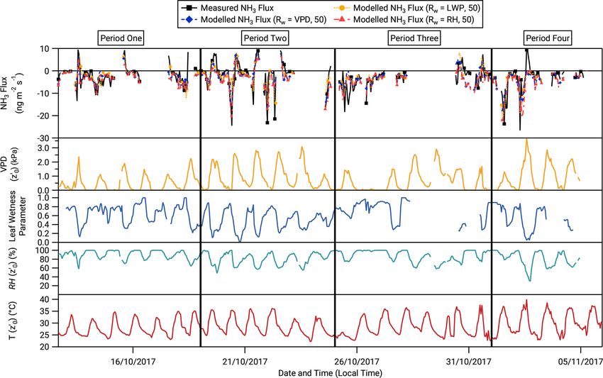
2810                                                          R. Ramsay et al.: Measurement and modelling of the dynamics

Even at deposition rates well below the saturation values, at-     resistances acting in series or in parallel impeding the ex-
mospheric Nr deposition can lead to changes in plant species       change. In the simplest model of bidirectional surface ex-
composition, with implication not only on biodiversity but         change, all exchange is approximated to occur via the leaf
also ecosystem services (Fowler et al., 2013). It is therefore     stomata situated at a single notional mean height (big-leaf
important that exchange models be developed for all major          approach) and is restricted by two atmospheric resistances in
biomes to accurately simulate NH3 deposition rates to forests      series (the aerodynamic resistance and quasi-laminar bound-
to predict potential environmental consequences.                   ary layer resistance), in series with a third (stomatal) resis-
    Ammonia is emitted in small quantities from (semi-             tance (stomatal compensation point model) (Sutton et al.,
)natural sources such as wild fires and the excreta of wild        1993).
animals, from plants as a result of non-zero NH+     4 concen-        Increasingly complex models include further pathways of
trations within the leaf apoplast, and from decomposing leaf       exchange (Kruit et al., 2010), with the most important for the
litter; both plant sources vary with the N status of the plants.   current study being the canopy compensation point model,
Of further importance for nitrogen modelling is therefore the      initially proposed by Sutton et al. (1995), which incorpo-
determination of the extent of potential emissions from for-       rates two parallel pathways of exchange at the canopy level
est ecosystems and the role such NH3 emission might play in        (Fig. 1). In the first pathway, a stomatal compensation point
the Nr cycle within natural forests. Forests were once consid-     (χs ) is introduced, which represents the concentration of NH3
ered to be perfect sinks for ammonia (Duyzer et al., 1992),        in the leaf stomata in (temperature-dependent) equilibrium
until bidirectional surface exchange of NH3 – i.e. deposi-         with the NH+   4 and pH of the apoplastic fluid. This stom-
tion to and emission from – was recorded in many stud-             atal compensation point controls the exchange of NH3 to and
ies of NH3 fluxes from forests (Langford and Fehsenfeld,           from the canopy to the leaf stomata, together with the associ-
1992; Neirynck and Ceulemans, 2008; Wyers and Erisman,             ated stomatal resistance (Rs ). In the parallel pathway, a unidi-
1998). Predominantly, this has been observed in forests situ-      rectional deposition flux is modelled from canopy to the leaf
ated close to sources of agriculturally derived Nr pollution,      cuticle, with a separate cuticular resistance (Rw ) controlling
although Hansen et al. (2015) also observed bidirectional          deposition. In a modified version of this model (the cuticular
fluxes over a more remote forest site.                             capacitance model), the leaf cuticle is considered to be both a
    The modelling of regional and local surface exchange of        sink and source for NH3 (Sutton et al., 1998). Here, the abil-
NH3 is based on parameterisations of the exchange, which           ity of water films on the leaf cuticle surface to act as a storage
remain unverified for many biomes of global importance due         of previously deposited NH3 is introduced as an analogue of
to the difficulty and cost of making measurements of NH3           an electrical capacitor, with emission fluxes of NH3 from the
fluxes. Datasets of NH3 flux measurements have mainly been         cuticle possible with the evaporation of charged water films.
limited to temperate agricultural and semi-natural ecosys-         Further models include ones which simulate the potential for
tems. Consequently, very little is known about the role of         soil and leaf litter below canopy to act as emission sources of
NH3 in the N cycling in remote ecosystems such as the trop-        NH3 (Nemitz et al., 2000; Sutton et al., 2009).
ics and their disturbance through anthropogenic activity. Al-         Using the static canopy compensation point model of NH3
though Flechard et al. (2015) identified the need for NH3 sur-     surface exchange, in combination with new NH3 flux and
face exchange measurements over tropical ecosystems, and           meteorological data measured at a remote, tropical rainforest
over rainforests in particular, such measurements have been        site, this study aims to present a series of local model formu-
limited so far. Here we present recent data from the Amazon        lations for χs and Rw which adequately simulate the bidirec-
Tall Tower Observatory site, situated in remote tropical rain-     tional fluxes of NH3 observed by Ramsay et al. (2020), with
forest, where NH3 fluxes were measured for 1 month during          a focus on the most suitable control metric for Rw . A statis-
the dry season of 2017 as part of a suite of species (Ramsay       tical comparison between models is conducted, with the aim
et al., 2020). This provides the data necessary to develop site-   to determine which parameterisation – and hence which of
specific parameterisations of NH3 surface exchange, with the       the factors controlling the formulation of model parameters –
potential for upscaling to the regional level. The companion       is best able to simulate observed fluxes. Discussion includes
paper (Ramsay et al., 2020) summarises the measured fluxes,        how meteorological conditions may have influenced model
including their statistics and average diurnal cycle, and dis-     performance and how subsequent studies of NH3 fluxes over
cusses the uncertainties associated with the measurement.          tropical rainforest may be conducted to help improve model
    As extensive reviews of NH3 surface exchange models are        performance. We discuss other model frameworks, such as
available (Flechard et al., 2015; Massad et al., 2010), only a     the dynamic CCP model, that could be used to simulate NH3
brief overview is provided here. Models of bidirectional NH3       bidirectional surface exchange in Sect. 4.1, with a focus on
surface exchange consider the control of fluxes to be analo-       the simplicity and performance of the static canopy compen-
gous to electrical resistances (Baldocchi, 1988; Monteith and      sation point (SCCP) model as justification for not pursuing
Unsworth, 2013). Whether emission occurs from the atmo-            more complex models further.
sphere to the canopy or vice versa is dependent upon the rel-
ative magnitude of ambient and canopy concentrations, with

Biogeosciences, 18, 2809–2825, 2021                                                   https://doi.org/10.5194/bg-18-2809-2021
R. Ramsay et al.: Measurement and modelling of the dynamics                                                                        2811

                                                                         rainforest. During convective daytime conditions, the flux
                                                                         footprint is much shorter, typically < 2 km.
                                                                            Measurements were made between 6 October and
                                                                         5 November 2017, during the region’s dry season. Lasting
                                                                         typically from August to November, the dry season is char-
                                                                         acterised by warmer, drier conditions in comparison to the
                                                                         wet season, which lasts from February to May. Air masses
                                                                         that arrive at the site during the dry season typically travel
                                                                         over some urban and agricultural areas located to the south
                                                                         and south-east of the site, which can give rise to periods of
                                                                         elevated black carbon (BC) and carbon monoxide (CO) con-
                                                                         centrations (Ramsay et al., 2020; Saturno et al., 2018).

                                                                         2.2     Measurements of ammonia and meteorological
                                                                                 parameters

                                                                         2.2.1    Ammonia

                                                                         Ammonia was measured using the Gradient of Aerosols and
                                                                         Gases Online Registration system (GRAEGOR), a semi-
                                                                         autonomous, continuous wet-chemistry instrument (ECN,
                                                                         the Netherlands) (Thomas et al., 2009). The GRAEGOR pro-
                                                                         vides online analysis of a suite of inorganic trace gases (NH3 ,
                                                                         HCl, HONO, HNO3 , and SO2 ) and their associated water-
Figure 1. Schematic of the canopy compensation point model of            soluble aerosol counterparts (NH+          −      −      −
                                                                                                              4 , Cl , NO2 , NO3 , and
Sutton et al. (1995). Ft , Fs , and Fw are, respectively, the total,     SO24 −) at two heights at hourly resolution. The instrument
stomatal, and cuticular fluxes of NH3 ; Ra , Rb , Rw , and Rs are, re-   consists of two sample boxes, which were set at two heights
spectively, the aerodynamic, quasi-laminar boundary layer, cuticu-       (z1 = 42 and z2 = 60 m) on the 80 m walk-up tower, with
lar, and stomatal resistances; and χa , χc , and χs are, respectively,
                                                                         a detector box which is connected to each sample box lo-
the atmospheric concentration of NH3 , the canopy compensation
                                                                         cated in an air-conditioned container at ground level for on-
point, and the stomatal compensation point.
                                                                         line analysis of samples.
                                                                            Each sample box contains a wet annular rotating denuder
2     Methodology                                                        (WRD) connected in series to a steam jet aerosol collec-
                                                                         tor (SJAC). A short section of high-density polyethylene
2.1    Field site description                                            (HDPE) tubing connects an inlet cone covered with an HDPE
                                                                         insect mesh to the sample boxes of the WRDs, ensuring
Measurements were conducted on an 80 m walk-up tower                     that losses of NH3 are minimised. The walls of each WRD
located at the Amazon Tall Tower Observatory site                        are coated in a constantly replenishing sorption solution
(2◦ 08.6370 S, 58◦ 59.9920 W). The Amazon Tall Tower Ob-                 of 18.2 M double deionised (DDI) water, with 0.6 mL of
servatory (ATTO) site lies on a level plateau 120 m above sea            H2 O2 (9.8 M) added per 10 L of sorption solution to elim-
level and is situated within a region of dense, undisturbed              inate potential biological contamination of the WRDs. Air
terra firme rainforest, with a mean canopy height of 37.5 m              is drawn simultaneously through both WRDs at a rate of
(Chor et al., 2017). The nearest large urban centre, Manaus,             16.7 L min−1 , kept constant by a critical orifice downstream
Brazil, is located 150 km to the south-west. A full descrip-             of the WRD. Unlike NH+      4 aerosol, gaseous NH3 diffuses
tion of the ATTO site, its permanent instrumentation, and the            through the laminar air flow onto the sorption solution coat-
floristic composition of the surrounding rainforest is given in          ing the walls of the WRD, and the solution is subsequently
Andreae et al. (2015).                                                   transported to the detector box at ground level for analysis.
   The rainforest extends homogenously for many hundreds                    The detector box contains a flow injection analysis unit
of kilometres to the north and east but gives way to shrub               (FIA) based on a selective ion membrane to analyse the con-
forest (campina) 5.5 km to the south, where the plateau de-              centration of NH3 within the WRD samples. WRD sam-
scends to meet the Uatumã River. The flux fetch require-                 ples are fed to the FIA unit, where NaOH (0.1 M) is first
ment for these gradient measurements with a geometric mean               added to the sample to form gaseous NH3 . The gaseous NH3
height of 50.2 m as determined from the approximation given              then passes through a semi-permeable polytetrafluoroethy-
by Monteith and Unsworth (2013) is 5.2 km. Therefore, NH3                lene (PTFE) membrane to enter a counterflow of DDI wa-
fluxes can be considered representative of a homogeneous                 ter to re-form NH+ 4 . The temperature-corrected conductivity

https://doi.org/10.5194/bg-18-2809-2021                                                         Biogeosciences, 18, 2809–2825, 2021
2812 R. Ramsay et al.: Measurement and modelling of the dynamics
of NH+ 4 is then measured in the conductivity cell of the FIA of measurement (Chor et al., 2017). The validity of this cor-
unit, from which the atmospheric concentration of NH3 at the rection was confirmed via the flux measurements of HNO3
height from which the sample was drawn can be determined. and HCl by Ramsay et al. (2020).
Through a valve control system within the detector box, the
WRD sample from each height is analysed for NH3 by FIA 2.4 Determination of concentrations and
once per hour, resulting in an hourly-resolved concentration meteorological parameters at the aerodynamic
gradient of NH3 . The FIA unit is calibrated autonomously mean canopy height
using three liquid NH+ 4 solutions (0, 50, and 500 ppb NH4
+
concentration), with the first calibration conducted 24 h after The aerodynamic resistance Ra and the quasi-laminar bound-
the GRAEGOR begins measurements and every 72 h after- ary layer Rb can be used to determine the temperature and
wards. Fresh standards were prepared prior to each calibra- NH3 concentration at the aerodynamic mean canopy height,
tion. A total of 10 autonomous calibrations were conducted z00 , if their respective values at a reference height are known
during this campaign. (Nemitz et al., 2009):
H
2.2.2 Meteorology Tz00 = T (z − d) (Ra (z − d) + Rb ) , (2)
ρcp
Wind speed (u), wind direction (wd), friction velocity (u∗ ), χz00 = χ (z − d) + Fχ (Ra (z − d) + Rb ) . (3)
and sensible heat flux were measured by a Gill WindMaster
mounted at 46 m on the 80 m walk-up tower. Relative humid- The relative humidity at z00 can be determined if the satu-
ity and air temperature were measured at 22, 36, and 55 m ration pressure at z00 (εsat (Tz00 )) and the water vapour pressure
using a series of Campbell HygroVUE™ temperature and at z00 (εz00 ) are known. εz00 can be calculated as
relatively humidity sensors. Net radiation and photosyntheti-
cally active radiation were measured at 75 m by, respectively, εz00 = ε(z − d) + FH2 O (Ra (z − d) + Rb ) , (4)
a net radiometer (Kipp and Zonnen NR-LITE2) and a quan-
tum sensor (Kipp and Zonnen PAR LITE). Hourly rainfall where FH2 O is the measured water vapour flux, as taken at
was measured using a HS Hyquest TB4-L. the 80 m tower. RHz00 is then calculated as
2.3 Modified aerodynamic gradient method εz00
RHz00 = × 100. (5)
In the constant flux layer over homogeneous surfaces, the εsat Tz00
flux of a chemical tracer χ can be determined using the aero-
dynamic method (AGM) if the vertical concentration gra- From measurements of Tz00 and RHz00 , the vapour pressure
dient of χ and its diffusion coefficient are known (Foken, deficit (VPD) in kilopascals (kPa) was determined.
2008). A modified form of the AGM – based on the verti-
2.5 Canopy resistance method
cal concentration difference (1c ) between measurements of
NH3 at 42 and 60 m, a series of stability parameters deter- The basic resistance model that describes deposition to a
mined from meteorological measurements, and u∗ as mea- non-perfectly absorbing surface approximates the ability of
sured at 46 m by eddy covariance (Flechard, 1998) – was the surface to regulate NH3 deposition through a canopy re-
used to determine the flux of NH3 as sistance, Rc , which can be calculated from the difference
1c between (a) the total resistance towards deposition (i.e. the
Fx = −u∗ κ , (1) inverse of the deposition velocity (Vd ) of NH3 at a refer-
z2 −d z2 −d z1 −d
ln z1 −d − 9H L + 9H L ence height) and (b) the sum of the atmospheric aerodynamic
where κ = 0.41 is the von Kármán constant and d is the zero- resistance, Ra , and the quasi-laminar boundary layer resis-
plane displacement height, determined as 0.9 hc = 33.4 m. tance, Rb (Fowler and Unsworth, 1979; Wesely et al., 1985):
The integrated form of the heat stability correction term, 9H , 1
is included to account for deviations from the log-linear wind Rc = − Ra (z − d) − Rb . (6)
Vd (z − d)
profile, while the term (z−d) / L is a dimensionless measure
of atmospheric stability, where L is the Obukhov length. Ra and Rb can be determined from Eqs. (7) and (8), respec-
The aerodynamic gradient method strictly holds for mea- tively (Garland, 1977; Ramsay et al., 2020):
surements made within the inertial sublayer. Corrections
must be applied to fluxes calculated using the AGM if mea- u(z − d) 9H (ζ ) − 9M (ζ )
Ra (z − d) = − , (7)
surements are made close to the canopy, within the rough- u2∗ κu∗
ness sublayer, as was the case in this study. Fluxes were cor-
rected using a correction factor, γF , whose magnitude was
determined from the stability conditions present at the time Rb = (Bu∗ )−1 , (8)
Biogeosciences, 18, 2809–2825, 2021 https://doi.org/10.5194/bg-18-2809-2021R. Ramsay et al.: Measurement and modelling of the dynamics 2813
where B is the sublayer Stanton number (Foken, 2008). How- where Ri represents the minimum bulk resistance stomatal
ever, this canopy resistance approach as outlined in Eq. (6) resistance for water vapour (for deciduous forest during sum-
can only successfully be applied if there is no bidirectional mer: Ri = 70 s m−1 ), St is the global radiation in watts per
exchange. Since both emission and deposition of NH3 were square metre (W m−2 ), and Tz00 is the temperature in degrees
observed in this study, a bidirectional exchange model was Celsius (◦ C) at the mean canopy height.
required to simulate surface atmosphere exchange of NH3 . The appropriateness of this parameterisation and the
The simplest bidirectional exchange model for NH3 is the choice of parameter Ri was evaluated against the water
static canopy compensation point (SCCP) model (Fig. 1) in vapour fluxes that were measured during fairly dry condi-
which the exchange between the canopy and the atmosphere tions when stomatal evapotranspiration is expected to be the
is controlled by a conceptual canopy compensation point dominant source.
(χc ). The bulk stomatal resistance (Rsb ) for water exchange can
In this SCCP model, the total surface–atmosphere ex- be calculated from the measured water vapour flux (FH2 O ) as
change of NH3 (Ft ) is the sum of two constituent fluxes, the (Nemitz et al., 2009)
unidirectional deposition of NH3 to the cuticle surface (Fw ),
and a bidirectional flux of NH3 through the leaf stomata (Fs )
(Sutton et al., 1995): εsat Tz00 − εz00
Rsb = . (14)
FH2 O
Ft = Fw + Fs , (9)
where To avoid periods during which sources other than evapo-
−χc transpiration contribute to the water flux, we applied a strin-
Fw = (10) gent filter criterion to exclude periods during or within 2 h
Rw
of rainfall or with RH > 80 %. This left fifty-five 30 min val-
and ues for the assessment. Measurement-derived values of Rsb
for H2 O were converted to the equivalent resistance for NH3 ,
(χs − χc )
Fs = . (11) accounting for the differences of the molecular diffusivities
Rs of the two gases (e.g. Hanstein et al., 1999), and the compar-
For the stomatal exchange flux, the difference between the ison was carried out on their reciprocal values (stomatal con-
notional mean concentration at canopy height (the canopy ductances, Gs and Gsb ), because it is the uncertainty in the
compensation point concentration (χc )) and the stomatal stomatal conductances that propagates directly into the pre-
compensation point concentration (χs ) provides the numer- dicted flux. A linear regression analysis revealed a very high
ator on the right-hand-side term in Eq. (11). When χs ex- R 2 value of 0.97 and a slope of 0.95 (using an intercept of 0),
ceeds χc , an emission occurs. χs is proportional to the ratio suggesting that the modelled resistances were slightly larger
of dissolved NH+ + but well within the range of the measurement uncertainty of
4 to H in the leaf apoplast (the apoplastic
ratio), which represents a dimensionless emission potential Rsb . Therefore, the parameterisation based on Wesely (1989)
(0), via a temperature function that describes the combined is appropriate for this site.
Henry solubility and dissociation equilibrium (Nemitz et al., This parallel cuticular pathway in the SCCP model treats
2004): the flux to the leaf cuticle (Fw ) to be unidirectional to a per-
fectly absorbing sink, given by the ratio of the canopy com-
161 500 10380 pensation point (χc ) and the cuticular resistance (Rw ). Rw
χs = exp − 0s . (12) has been described successfully by a number of empirically
T T
derived parameterisations in various studies as outlined by
Here, T is the temperature of the canopy in kelvin (K). Massad et al. (2010), with most using either relative humid-
The stomatal resistance, Rs , is primarily dependent on ity or water vapour pressure deficit as proxies for the ability
global radiation (St ), with additional potential influences of NH3 to absorb to the leaf surface. The term Rw is dis-
from factors such as temperature, vapour pressure deficit, and cussed further in Sect. 3.4.
leaf and root water potentials. Here the generalised function The canopy compensation point (χc ) is the conceptual
for bulk stomatal resistance as per Wesely (1989) with the mean concentration of NH3 inside the canopy, at which the
parameters recommended for tropical vegetation is used to stomatal, cuticular, and above-canopy fluxes balance each
calculate the stomatal resistance for NH3 (Rs (NH3 )): other. It is therefore dependent upon the ambient concen-
2 tration of NH3 (χa ) and various physical and chemical pa-
Rs (NH3 ) =Ri 1 + 200(St + 0.1) −1 rameters, both on the surface of the leaf and the surrounding
atmosphere, as described by the resistances (stomatal, cu-
i−1
h ticular, aerodynamic, and quasi-laminar boundary layer) and
400 Tz00 400 − Tz00 , (13) the stomatal compensation point previously described. In this
https://doi.org/10.5194/bg-18-2809-2021 Biogeosciences, 18, 2809–2825, 20212814 R. Ramsay et al.: Measurement and modelling of the dynamics
study, χc was calculated as to give a leaf wetness parameter (LWP) whose values range
from 0 (dry) to 1 (wet).
χs × Rw × (Ra + Rb ) + χa × Rw × Rs
χc = . (15)
Rw × Rs + Ra + Rb × Rw + Ra + Rb × Rs
3 Results
Prompted by the observation of morning emissions of NH3
3.1 Temperature, relative humidity, VPD, and LWP at
which could not be explained by stomatal exchange alone,
canopy
this model was further extended by Sutton et al. (1998) to
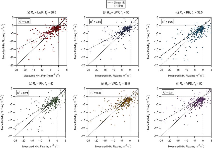
account for bidirectional exchange with leaf surfaces, by al- The time series of calculations of Tz00 , RHz00 , and V P Dz00 ,
lowing NH3 to be absorbed and desorbed to/from leaf wa- together with measurements of the leaf wetness parameter
ter layers. The extended model calculated the NH3 holding and measured and modelled fluxes of NH3 (see Sect. 3.2 be-
capacity by estimating the leaf water amount in relation to low), are shown in Fig. 2. The measurements can broadly
RH. The ammonia holding capacity was implemented into be split into four distinct periods of warmer, drier conditions
the resistance framework by considering it analogous to an and cooler, wetter conditions. Period One, from 6 to 18 Oc-
electric capacitor. The charge of this “capacitor” depended tober, is typified by an average leaf wetness at the canopy
dynamically on previously deposited NH3 and tended to be of 0.7, with an average RH of 82 %, suggesting the preva-
released as dew dried out in the morning. Similarly, Nemitz lence of humid, wet conditions. Period Two extends from 19
et al. (2001) extended the model by a second model layer to to 25 October, where leaf wetness at the canopy decreases
describe additional exchange with the ground level or soil. while VPD increases, which is paired with a drop in aver-
age RH. Conditions resume the same pattern as Period One
2.6 Leaf wetness measurements during Period Three, which lasts between 26 October and
1 November but gives way to drier, warmer conditions (Pe-
Leaf surface wetness was measured using a sensor array as riod Four) from 2 November until the end of the campaign.
described in Sun et al. (2016), which was based on the de- A distinct lag exists between the relative humidity at the
sign by Burkhardt and Eiden (1994). Six sensors arranged canopy level and the leaf wetness measurements, particularly
in pairs of two, each consisting of gold-plated electrodes ar- during the drier conditions from 19 to 25 October. RH min-
ranged as a clip, were each attached to a leaf situated 27 m ima, which occur on average between 11:00 and 13:00 (all
above ground level and within the canopy surrounding the times presented in this work are given as local time: Amazon
80 m walk-up tower. Each clip provided a measurement in time, UTC−4), are not reflected in leaf wetness measure-
millivolts (mV) that was related to the electrical conductiv- ments until several hours later. Minima leaf wetness mea-
ity between the two electrodes. Data were recorded using a surements during this period are recorded between 13:00 and
Raspberry Pi 2 Model B (Raspberry Pi Foundation, Cam- 16:00.
bridge) at a temporal resolution of 1 min. The sensor array
was checked daily to ensure good contact between the clips 3.2 Overview of NH3 measurements
and the leaf. Leaf wetness was measured from 6 October to
5 November 2017. Unlike conventional (binary) wetness grid Figure 2 shows the time series of the measured fluxes to-
sensors, this approach provides some gradation between fully gether with model results (see below). Both (positive) emis-
dry and fully wet canopies. sion and (negative) deposition fluxes were recorded during
Raw values from each sensor pair were converted to a the campaign, ranging from +9.5 to − 30.2 ng m−2 s−1 . Fig-
leaf wetness parameter value, ranging from 0 to 1, according ure 3 presents calculated NH3 fluxes as scatter plots for the
to the methodology outlined by Klemm et al. (2002). Dur- duration of the campaign against paired canopy values of
ing periods of significant precipitation (≥ 0.1 mm rainfall per temperature and relative humidity as well as the leaf wet-
hour), the leaf is considered fully wet and the raw signal from ness parameter. Shaded contour areas – from green to red for
the sensor is at a maximum value. During prolonged dry pe- low to high density of measurements – are added to the scat-
riods the leaf is considered to be dry, and the lowest recorded ter plots to highlight temperature, relative humidity, and leaf
conductivity of the sensor pair during these periods is desig- wetness conditions where measurements of NH3 fluxes were
nated as a “zero signal”. The net signal from each sensor pair particularly concentrated. A statistical summary of linear re-
is determined by subtracting the corresponding zero signal gression models for calculated NH3 flux and the respective
from the raw signal for each period of data considered. The parameter plotted is given for each subplot in Fig. 3.
cumulative time period of precipitation is then determined While emission and deposition occur across the full range
from rainfall measurements. For this study, precipitation oc- of temperatures recorded during the campaign, a weak corre-
curred during 15 % of the total campaign time. Consequently, lation (R 2 = 0.02; p = 0.02) in the linear regression model
the signal percentile for each sensor that represents periods of NH3 flux against temperature suggests that emissions were
of precipitation was 85 % in this study. Finally, the zero cor- more likely to be observed during warmer conditions. Rela-
rected net signals are divided by the value of signal percentile tive humidity appears to be a somewhat stronger driver of
Biogeosciences, 18, 2809–2825, 2021 https://doi.org/10.5194/bg-18-2809-2021R. Ramsay et al.: Measurement and modelling of the dynamics 2815 Figure 2. Time series of (from top to bottom) measured and modelled NH3 fluxes, vapour pressure deficit at z00 , leaf wetness parameter, relative humidity at z00 , and air temperature at z00 throughout the period of NH3 flux measurements. Figure 3. Scatter plots with line of best fit and data density shadings for NH3 flux against (from a to c) relative humidity at z00 , temperature at z00 , and leaf wetness parameter. NH3 surface exchange behaviour (R 2 = 0.08; p = 3.98 × periods when the leaf surface is wet (> 0.6) or completely 10−4 ) than temperature. The slope and density contours sug- saturated 1 (Fig. 2). gest that emissions are more likely as relative humidity de- creases. The strongest predictor of the three meteorologi- 3.3 Determination of stomatal compensation points cal parameters investigated is the leaf wetness parameter and emission potentials (R 2 = 0.19; p = 2.72 × 10⁻⁵ ). Emissions predominately oc- cur during periods when leaf wetness parameter values fall One of the elements of modelling of NH3 flux through the below 0.5, with deposition occurring predominately during static canopy compensation point model is the stomatal flux https://doi.org/10.5194/bg-18-2809-2021 Biogeosciences, 18, 2809–2825, 2021
2816                                                               R. Ramsay et al.: Measurement and modelling of the dynamics

                                                                           Equation (12) can therefore be rearranged to give an ex-
                                                                        pression for 0s that is dependent upon Tz00 and χs , where χs
                                                                        can be substituted with a value of χa at which a sign change
                                                                        in the flux of NH3 occurs:
                                                                                                       1
                                                                        0s =                                        .          (16)
                                                                                 161500
                                                                                 Tz0 +273   exp       − T10380        1
                                                                                                                      χs
                                                                                   0                     z0 +273
                                                                                                           0

                                                                        Using the values of χa measured in this campaign that are
                                                                        inferred to be equal to χs , the apoplastic ratio applicable to
                                                                        the period of measurement was determined as 38.5 ± 15.8.
                                                                        Also shown in Fig. 4 is the temperature response curve of
                                                                        χs consistent with this value of 0. Consequently, modelled
                                                                        values of χs based on a value of 0s = 38.5 were determined
                                                                        for the campaign period and subsequently used to determine
                                                                        values of χc and total modelled flux. As this value resulted
                                                                        in an under-prediction of the peak emissions, an alternative
                                                                        enhanced value of 0s = 50 was also explored to develop fur-
                                                                        ther parameterisations for comparison. By using an enhanced
Figure 4. Estimating the stomatal compensation point from the am-
                                                                        value for 0s , all emissions from the leaf surface are implicitly
bient NH3 concentrations at which the flux changed signs as a func-
tion of the temperature at z00 . The black dotted line shows the tem-
                                                                        considered to originate from leaf stomata rather than cuticu-
perature response curve calculated using an apoplastic ratio of 38.5,   lar desorption or other potential sources of NH3 emissions,
while the red dotted line shows the temperature response curve cal-     such as soil or leaf litter.
culated using a ratio of 50.
                                                                        3.4   Determination of Rw parameterisations based on
                                                                              three alternative proxies for leaf water volume
(Fs ), which, from Eq. (11), depends on the canopy concentra-
tion of NH3 (χc ) and the stomatal compensation point (χs ).            Considering the observed drivers for NH3 surface exchange
The value of χs is determined by the leaf surface temperature           discussed in Sect. 3.2, three different parameterisations for
(in this study, taken as Tz00 ) and the apoplastic ratio (0s ). If      the cuticular resistance Rw were developed for this study,
0s is known, which varies with vegetation type (Hoffmann                based upon three alternative proxies of the NH3 holding ca-
et al., 1992; Mattsson et al., 2009), environmental stressors           pacity of the leaf water layers: RHz00 , V P Dz00 , and leaf wet-
such as drought (Sharp and Davies, 2009), and nitrogen nu-              ness. Subsequently, each parameterisation of Rw was used
trition (Massad et al., 2008), then χs and subsequently Fs can          to develop three distinct values for Fw , the unidirectional
be modelled. The fact that emissions at this site regularly oc-         flux component of the cuticular-resistance-based single-layer
curred during midday (when Tz00 is at its maximum) and were             model, each describing the surface atmosphere exchange of
related to drier, warmer conditions (Fig. 3) is consistent with         NH3 at the ATTO site.
the emission flux originating from the stomata.                            The first parameterisation was based on measurements of
   0s can be inferred from measurements during conditions               RHz00 using the following equation (Sutton et al., 1993):
where the NH3 surface exchange is judged to be dominated
                                                                                         100 − RH

by stomatal exchange, with a negligible contribution from               Rw = α + exp                  .                              (17)
                                                                                             β1
desorption of NH3 from the leaf surface.
   Under conditions where Rw is very large compared with                   Here, α determines the minimum cuticular resistance
Rs , the ambient NH3 concentration (χa ) at which a zero net            (which is α = 1 s m−1 ), while β1 is a constant scaling co-
flux occurs (i.e. when the difference between χc and χs is 0)           efficient controlling the increase of Rw with decreasing rela-
is implicitly equal to χc and χs . Therefore, if NH3 surface            tive humidity. The coefficients α and β1 were fitted by least-
exchange is driven by stomatal exchange, χs may be deter-               squares optimisation between total modelled and observed
mined from the values of χa at which the flux changes from              values of NH3 flux taken during the campaign to arrive at
deposition to emission, or vice versa (Nemitz et al., 2004).            values of α = 2 s m−1 and β1 = 9, which were used for mod-
Figure 4 presents the ambient NH3 concentrations measured               elling Rw based on RHz00 for the entirety of the campaign.
during the campaign at which such flux sign changes occur as            The second parameterisation was based on measurements of
a function of Tz00 for conditions under which Rw is expected            the vapour pressure deficit, using a formulation for Rw based
to be fairly large (RH < 60 %).                                         upon that employed by Flechard et al. (1999):

                                                                        Rw = α + β2 expγ1 (VPD) .                                 (18)

Biogeosciences, 18, 2809–2825, 2021                                                               https://doi.org/10.5194/bg-18-2809-2021
R. Ramsay et al.: Measurement and modelling of the dynamics 2817
As with the parameterisation of Rw in Eq. (17), the coef- 38.5 differ more from the observed values than those which
ficient α is the minimum value for Rw at zero VPD, set at use an apoplastic ratio of 50 (near 1 standard deviation from
2 s m−1 . β2 and γ1 are constant scaling coefficients which, calculated). Modelled daytime values tend to differ less from
respectively, control the scaling of the exponential term and their corresponding observed value in comparison to night-
the scaling of the vapour pressure deficit response. Through time values. Modelled values during Period One have the
least-squares optimisation, a value of 5 was chosen for β2 least divergence from the observed overall (day and night),
and 1.7 for γ1 for the determination of Rw based on Eq. (18) while the greatest divergence in modelled values occurs dur-
for the entirety of the campaign. ing Period Four, particularly at night. For model b, 91 % of
Finally, a novel parameterisation for Rw based upon mea- values agree with the observed direction of fluxes, and it is
surements of leaf wetness was developed for this campaign the best performing model using this parameter. Conversely,
based on least-squares optimisation: model c values agree with only 83 % of the observed direc-
h i tion of fluxes.
Rw = α + β3 expγ2 (1−LW P ) − 1 . (19) Figure 2 shows the full time series of modelled NH3 fluxes
from models b, d, and f alongside the measured flux. In gen-
As with the parameterisations of Rw described in Eqs. (17) eral, periods of emission and deposition are modelled well
and (18), α is the minimum value of Rw at maximum leaf by all three models, with two exceptions: the emission pe-
wetness, set at 2 s m−1 ; β3 is a scaling coefficient, similar riod from 12:00 to 16:00 on 30 October, where modelled
to that of the parameterisation in Eq. (18), set at a value fluxes suggest an earlier emission from 11:00 which lasts for
of 5; and γ2 is a scaling coefficient controlling the increase fewer hours; and from 13:00 to 15:00 on 2 November, where
in Rw with the decrease in leaf wetness, set in this study no model predicts an emission, in contrast to the measure-
to 4.8. With this parameterisation, Rw approaches α for a ments. The magnitude of modelled fluxes generally agrees
fully wet canopy and is capped at Rw = 605 s m−1 for a fully well with the observed flux, although model d, which uses an
dry canopy. Rw parameterisation based on RH, tends to estimate smaller
emissions in comparison to model f (Rw = VPD). Model b
3.5 Comparison of modelled with observed NH3 fluxes (Rw = LWP) comes closest to replicating the magnitudes of
the measured emissions, although as with the other two mod-
Six discrete model runs of NH3 surface exchange were inves- els it underestimates the magnitude of the measured deposi-
tigated, via Eqs. (9), (10), and (11), using the two values of tion.
the apoplastic ratio (0s = 38.5 and 0s = 50) combined with
one of the three parameterisations for Rw (relative humidity, 3.6 Error in observed and simulated fluxes
RH; vapour pressure deficit, VPD; and leaf wetness parame-
ter, LWP) described above. These models are The errors in the observed fluxes of NH3 during this cam-
paign are presented in Ramsay et al. (2020). Using a Gaus-
a. Rw = LWP, 0s = 38.5,
sian error propagation approach, a median percentage error
b. Rw = LWP, 0s = 50, of 33 % was calculated for the observed NH3 fluxes.
The error in the simulated fluxes can also be determined
c. Rw = RH, 0s = 38.5, using an error propagation method. Equation (9) highlights
d. Rw = RH, 0s = 50, that the total simulated flux (Ft ) is the sum of the cuticular
flux (Fw ) and the stomatal flux (Fs ). The total uncertainty in
e. Rw = VPD, 0s = 38.5, and Ft , σFt , can therefore be determined by
f. Rw = VPD, 0s = 50. q
σFt = σFw 2 + σFs 2 , (20)
Table 1 presents a summary of the model results, with
average mean modelled fluxes for the overall campaign, where σFw and σFs are the associated errors in, respectively,
together with day- (06:00–17:00) and night-time (18:00– Fw and Fs . In turn, σFw and σFs can be calculated using a
05:00) average mean values for the four separate periods of Gaussian error propagation based on Eqs. (10) and (11) re-
the campaign discussed in Sect. 3.1. Also presented are av- spectively, which rely on the errors in Ra , Rb , Rs , and Rw
erage mean values for calculated fluxes based on NH3 mea- measurements.
surements during the campaign and the percentage of mod- While the error in Fs will remain the same for all simulated
elled values which agree in flux direction with observed val- values of Ft , the error in Fw will vary on the choice of Rw pa-
ues. Modelled mean values highlighted in bold signify where rameterisation. Thus, the error in Rw is the primary variable
the model value deviates by more than 25 % from the corre- which governs the differences in the error in Ft between the
sponding observed mean. The models which differ least and simulated values.
most from the observed values are models b and c, respec- Using this framework, the error values were calculated for
tively. Models which use the calculated apoplastic ratio of each Rw and 0s parameterisation for the simulated total flux.
https://doi.org/10.5194/bg-18-2809-2021 Biogeosciences, 18, 2809–2825, 20212818 R. Ramsay et al.: Measurement and modelling of the dynamics
Table 1. Summary of model results, with comparison to measured hourly NH3 fluxes (in ng m−2 s−1 ). Presented are the overall mean
average flux for measured and modelled NH3 fluxes (with associated errors), the correctness of modelled flux direction in comparison to
the measured values, and mean average values for modelled and measured NH3 fluxes during day (06:00–17:00) and night (18:00–05:00)
for the four periods of the measurement campaign. Values in bold signify average model values which differ by ± 25 % from corresponding
measured average values.
Overall Correctness Period One Period Two Period Three Period Four
of direction day night day night day night day night
(%)
Measured −2.83 ± 0.94 – −2.80 −1.47 −3.36 −2.14 −4.74 −1.97 −6.61 −2.02
Model a Rw , LWP, 38.5 −3.03 ± 0.48 87.2 −3.19 −1.86 −3.33 −2.81 −4.55 −2.58 −5.99 −2.90
Model b Rw , LWP, 50 −2.69 ± 0.49 90.6 −2.36 −1.86 −3.25 −2.80 −3.93 −2.37 −5.94 −2.89
Model c Rw , RH, 38.5 −3.97 ± 0.51 82.4 −4.76 −2.45 −5.05 −3.74 −6.35 −3.52 −4.28 −2.76
Model d Rw , RH, 50 −3.73 ± 0.56 86.8 −4.14 −2.45 −4.15 −3.73 −5.89 −3.52 −4.22 −2.75
Model e Rw , VPD, 38.5 −3.48 ± 0.62 84.8 −3.45 −2.28 −3.55 −3.58 −4.62 −3.32 −5.83 −3.35
Model f Rw , VPD, 50 −3.16 ± 0.61 89.1 −2.64 −2.28 −2.50 −3.58 −4.01 −3.32 −5.78 −3.34
In the overall calculated total flux in Table 1, the associated compensation point model (SCCP) was unable to simulate
error, in ng m−2 s−1 , is also shown. their observed emissions.
At ATTO, there is no indication that the single-layer SCCP
model was unable to reproduce the temporal dynamics of
the measured NH3 surface exchange. Indeed, an exploratory
4 Discussion application of the dynamic CCP model did not result in an
improvement in model performance, and therefore the mod-
4.1 Temporal dynamics elling work here focused on the static model as a simpler ap-
proach able to reproduce the measurements. The absence of
The observed bidirectional surface exchange of NH3 from a morning desorption peaks at the ATTO forest is likely due to
remote tropical rainforest site was modelled using a series of the small night-time adsorption of NH3 into leaf water layers
canopy compensation point, cuticular-resistance-based mod- associated with the low night-time NH3 concentrations at this
els using a variety of different Rw parameterisations and site. Dry deposition of aerosol ammonium nitrate (NH4 NO3 )
apoplastic ratios. is another source of volatile NH+ 4 on leaf surfaces, and con-
As highlighted in the Introduction, measurements of NH3 centrations of this compound are again typically very small
surface exchange over natural ecosystems such as forests in Amazonia (Wu et al., 2019). In addition, given the high
remain sparse. This is particularly true for measurements RH, the water layers may not dry out as rapidly and com-
over remote environments such as tropical vegetation. To pletely as at other sites. The measured median NH3 atmo-
our knowledge, there have not been any direct flux mea- spheric concentration at the canopy height during the mea-
surements over tropical vegetation to date, although Trebs surement period was 0.23 µeq m−3 , with an estimated annual
et al. (2004) and Adon et al. (2010, 2013) inferred fluxes total reactive N dry deposition input of 1.74 kg N ha−1 yr−1
from single point concentration measurements. Exchange of (Ramsay et al., 2020). This is far lower than reported by
NH3 has been measured previously at temperate forest sites Neirynck and Ceulemans (2008) and by Wyers and Erisman
and reported to be bidirectional: for example, Langford and (1998), both of whose sites were subject to high levels of
Fehsenfeld (1992) noted daytime emission from a remote agricultural pollution. As noted by Massad et al. (2010) and
forest near Boulder, Colorado; Neirynck and Ceulemans Zhang et al. (2010), higher atmospheric inputs of N to for-
(2008) observed bidirectional NH3 exchange (with median est systems lead to an increase in the stomatal emission po-
diel emissions recorded between 12:00 and 16:00) over a tential. Conversely, with lower atmospheric NH3 concentra-
Scots pine (Pinus sylvestris) forest in Flanders, Belgium; and tions, the potential for forests to act as a source of NH3 is in-
Wyers and Erisman (1998) noted daytime emissions from a creased, as the likelihood of the canopy compensation point
Douglas fir (Pseudotsuga menziesii) forest at Speuld in the exceeding the ambient concentration increases. The low N
Netherlands. When using models to determine the drivers of status of the tropical vegetation may also favour transfer of
surface exchange above forest sites, these studies often stress N absorbed to the cuticle into the leaf, e.g. via liquid films
the importance of cuticular desorption as a further process that extend from the cuticle into the stomata (Burkhardt et al.,
that dominated in the morning when emission could not have 2012).
originated from stomatal compensation points. Indeed, in the In general, the fluxes measured at ATTO could also be re-
case of Neirynck and Ceulemans (2008), the static canopy produced without including a further soil layer, potentially
Biogeosciences, 18, 2809–2825, 2021 https://doi.org/10.5194/bg-18-2809-2021R. Ramsay et al.: Measurement and modelling of the dynamics 2819
with one exception (see below). Such a layer is needed where tions, values of 0s can be as low as 5–10 (Hanstein et al.,
night-time emissions are observed that are clearly not under 1999). The species of vegetation is also critical (Mattsson
stomatal control (Nemitz et al., 2000; Hansen et al., 2017). et al., 2009). Plants which are reliant on mixed nitrogen
The consistently warmer noon-time conditions at the leaf sources (ammonium, nitrate, and organic N), and which are
canopy during measurements at the ATTO site would also more reliant on root rather than shoot assimilation of nitro-
favour stomatal-exchange-driven emissions of NH3 . An in- gen, exhibit lower apoplast ratios than nitrate-reliant, shoot-
crease in leaf temperature, with VPD controlled for, has assimilating species (Hoffmann et al., 1992). The value of
been shown to lead to greater gas exchange through in- 38.5 which was inferred from measurements lies in the range
creased stomatal openings (Urban et al., 2017), while alter- of 0s values exhibited by semi-natural vegetation with low N
ations to the Henry and dissociation equilibria would lead inputs and in the lower range of overall forest values quoted
to a change in the stomatal compensation point favouring by Massad et al. (2010).
increased stomatal emissions. Similarly, the unstable con-
ditions at noon above the canopy over tropical rainforest 4.3 Model performance with respect to Rw
lead to reductions in Ra , which would increase any emis- parameterisation
sions occurring at the time that were driven by stomatal ex-
change (Flechard et al., 2015). In the study of forest NH3 An assessment of the performance of the individual parame-
emissions that is most similar in ambient NH3 concentra- terisations against calculated NH3 fluxes is included in Fig. 5,
tions, canopy compensation points, and apoplast ratios to this which displays the results of simple linear regression mod-
study, Hansen et al. (2017) come to a similar conclusion on els for the simulated values of each NH3 flux model against
the observed daytime emissions from a remote, temperate observed NH3 fluxes. With regards to the Pearson correla-
forest in Indiana, USA. tion coefficient (r), the rank of models from most strongly
Despite the low N inputs and apoplastic NH+ +
4 / H ra- correlated with observed NH3 fluxes to least correlated is
tio, significant emission periods were observed above the model b, model a, model f, model e, model d, and model c
ATTO site. One driver is clearly the high daytime leaf tem- (model descriptions are found in Table 1). The Rw parame-
perature. The average flux amounted to a small deposition terisation was a stronger determinant of model–measurement
of − 2.8 ng m−2 s−1 suggesting that, on average, the site re- correlation than the choice of 0. Correlation with measure-
ceives more N as NH3 than it loses. Possible sources include ments is highest for the models using an Rw based upon LWP,
small-scale farming and biomass burning. followed by those which use VPD and finally RH. Within
each grouping, models using 0 = 50 provide simulated val-
4.2 Apoplast ratio ues that have a better correlated fit with observed values than
0 = 38.5. Overall model performance is in many ways more
The apoplastic ratio of NH+ +
4 / H (0s ) inferred from the sensitive to Rw than 0 as is apparent from the Taylor dia-
measurements in this study was 38.5 ± 15.8; the models in- gram (Fig. 6), which summarises in one diagram the three
vestigated used either a value of 38.5 or 50 (close to 1 stan- complementary model–measurement performance statistics
dard deviation from inferred value). Both values are signifi- of the (i) correlation coefficient (r), (ii) centred root mean
cantly lower than the majority of 0s values obtained for other squared error (RMSE), and (iii) within-model and within-
forest sites. Wang et al. (2011) give a value of 0s = 400 measurement standard deviations (SD) (Taylor, 2001). The
for green temperate forest canopies, which is also used by statistical metrics visualised in Fig. 6 are summarised in Ta-
Hansen et al. (2017). Massad et al. (2010) review a range ble 2.
of 0s values derived from measurements of NH3 surface ex- The standard deviation in the observed flux dataset is
change over forest, which range from 0s = 27 (as measured 3.65 ng m−2 s−1 . The model that comes closest to replicat-
directly through bioassay for unfertilised Spruce forest) to ing this same variability is model b (2.65 ng m−2 s−1 ), with
0 = 5604 as determined by Wyers and Erisman (1998) for model e (2.24 ng m−2 s−1 ) replicating observed values least
a highly polluted P. menziesii forest. The study by Neirynck well, although the overall range between model standard de-
and Ceulemans (2008) used a value of 3300 in spring and viation is broadly similar. It should be borne in mind, how-
1375 in summer for a P. sylvestris forest. ever, that the standard deviation of the measured flux includes
The disparity in the emission potentials (the apoplastic ra- measurement uncertainty in addition to real variability, as do
tios) between other forest sites and the tropical rainforest the modelled values, which are based on measured param-
site at ATTO is again linked to nitrogen input. With larger eters. With regards to r, model b simulated values produce
N inputs where nitrogen is deposited in excess, the stomatal the highest correlation with the observed values at r = 0.71,
concentration is increased (Schjoerring et al., 1998). Con- in comparison to model c, which performs the worst at r =
sequently, at polluted areas such as the forest sites stud- 0.45. Finally, the model with the lowest root mean square er-
ied by Neirynck and Ceulemans (2008), apoplastic ratios ror from the observed is model b at 2.79 ng m−2 s−1 , with the
are increased, while at sites with lower N input, such as highest error found in model c, at 3.31 ng m−2 s−1 . There-
semi-natural vegetation with low ambient NH3 concentra- fore, from the ability of the parameterisations to reproduce
https://doi.org/10.5194/bg-18-2809-2021 Biogeosciences, 18, 2809–2825, 20212820 R. Ramsay et al.: Measurement and modelling of the dynamics Figure 5. Linear regressions between measured NH3 fluxes and six models (a–f) of NH3 fluxes differing in the approach used to derive a value for the cuticular resistance Rw and in the value used for the apoplastic ratio 0, as noted above each panel. the measured average fluxes as presented in Figs. 5, 6, and and ranges in a fairly narrow band between 100 % and 80 %, (Table 1), it can be concluded that parameterisation b, in leaf wetness reaches minima between 13:00 and 16:00 and which the value Rw is parameterised using leaf wetness pa- can decrease significantly, particularly during Period Two of rameter values and where the apoplastic ratio is set to 50, the campaign. is the best performing model in simulating NH3 surface– Overall, the results indicate that there is significant value atmosphere exchange at the ATTO site, while model c is the for interpreting field measurements in making direct mea- worst performing. surements of leaf wetness using leaf wetness clip sensors of Although the leaf wetness parameter measured with the the type used here. Although leaf wetness or surface wetness leaf clip sensors is somewhat empirical, it is not surpris- measurements are not typically available for use in chem- ing that it appears to reflect the actual leaf water amount istry transport models, canopy wetness is often simulated by more closely than the proxies via VPD and RH. All three land surface models (Katata et al., 2010) and within chemical parameters should be closely linked. Even after optimisation transport models (Campbell et al., 2019). Simulated surface of the models, however, extensive differences in model out- wetness data, as a leaf wetness parameter, could therefore put remain, principally between the models using leaf wet- be used to model NH3 fluxes using the LWP-dependent Rw ness parameter and RH as model inputs. Figure 7 presents parameter as described here. Alternatively, VPD-based pa- a scatter plot of leaf wetness measurements against RH nor- rameterisations, over RH-based parameterisations, could be malised to the canopy height. The relationship between them employed instead. is best described through a power equation, which suggests that leaf wetness decreases more sharply than RH across the campaign. Indeed, Fig. 2 shows a distinct lag between ob- served RH (as well as VPD) and the leaf wetness parameter. While RH minima are detected between 11:00 and 13:00, Biogeosciences, 18, 2809–2825, 2021 https://doi.org/10.5194/bg-18-2809-2021
R. Ramsay et al.: Measurement and modelling of the dynamics                                                                        2821

Table 2. Summary of model statistical performance (correlation coefficient R, centred root mean square error, and standard deviation) as
presented in Fig. 6.

                                                                   R         RMSE      Standard deviation
                                                                                            within model
                                                                       (ng m−2 s−1 )        (ng m−2 s−1 )
                              Model a. Rw , LWP, 0 = 38.5      0.69            2.81                  2.49
                              Model b. Rw , LWP, 0 = 50        0.71            2.79                  2.65
                              Model c. Rw , RH, 0 = 38.5       0.45            3.31                  2.60
                              Model d. Rw , RH, 0 = 50         0.46            3.27                  2.62
                              Model e. Rw , VPD, 0 = 38.5      0.62            2.92                  2.24
                              Model f. Rw , VPD, 0 = 50        0.64            2.90                  2.49

                                                                       validity of equating χa to χc only holds for dry conditions
                                                                       (e.g. RH < 50 %), when Rw can reliably be expected to be
                                                                       large. At higher humidity values, leaf cuticles may start to
                                                                       become a small sink, and χc becomes an underestimate of
                                                                       χs . At the ATTO site, where median humidity at the canopy
                                                                       level throughout the campaign was 87 %, with only a few
                                                                       occurrences during the drier Period Two and Period Four
                                                                       where it fell below 60 %, this approach of inferring 0s from
                                                                       NH3 measurements was likely affected. However, the impact
                                                                       does not appear to have completely invalidated the use of
                                                                       the method, as the somewhat larger value of 50 that resulted
                                                                       in models with best agreement still lies within 1 standard
                                                                       deviation of the inferred 0s value. An accurate determina-
                                                                       tion of apoplastic ratio for tropical rainforest, derived from
                                                                       leaf assays, would improve the accuracy of the model and
                                                                       therefore remains an important area for future investigation.
                                                                       However, its variability across the large plant species diver-
                                                                       sity would likely provide a challenge in deriving a bottom-up
Figure 6. A Taylor diagram summarising the statistical compar-         mean value that governs the net exchange.
isons between the modelled NH3 fluxes from the six models a–f
described in the text and the measured NH3 fluxes.
                                                                       4.5   Temporal variability in model performance

                                                                       Modelled values diverge significantly from observations at
4.4   Model performance with respect to the choice of                  several points during the campaign. In particular, on 30 Oc-
      stomatal emission potential                                      tober every model predicts an earlier, less sustained emission
                                                                       in comparison to the observation, while on 2 November, no
As is visually apparent in Fig. 7, the influence of the apoplas-       model predicts any emission, contrary to observations, which
tic ratio is relatively minimal for reproducing flux variability       suggest a strong emission of NH3 from 13:00 to 15:00. With
in comparison to the effect of Rw parameterisation over the            regards to the divergence in models from the observations on
0s range explored (38.5 to 50). However, the choice of 0               2 November, the possibility of other sources of NH3 emis-
does affect the model’s ability to reproduce the overall mag-          sion that would not be accounted for using the single-layer
nitude of the fluxes during daytime (Table 2).                         model could be considered. For example, from the evening
   Models that used the 0s value of 50 (the upper bound to the         of 31 October to the early morning of 2 November, heavy
inferred values of 38.5 for 0s ) (b, d, and f) simulated values        precipitation periods were recorded, coupled with increased
better in agreement with observations in comparison to their           deposition fluxes of NH3 on 1 November. Increased wet de-
paired Rw models (respectively, a, c, and e) which used the            position of N through NH+    4 in rainwater and washed from the
value of 38.5. In particular, the use of 38.5 as a value led to        canopy (Nemitz et al., 2000) to the forest floor or the higher
models underestimating the scale of the emissions.                     soil moisture itself could have led to an increase in soil or leaf
   The discrepancy highlights a potential problem with us-             litter microbial activity below canopy. Subsequent drying of
ing the method of inferring 0s as outlined in Sect. 3.3 in             the soil and leaf litter throughout 2 November might have led
tropical conditions. As outlined by Nemitz et al. (2004), the          to an evaporation of NH3 from the litter or soil layer from

https://doi.org/10.5194/bg-18-2809-2021                                                        Biogeosciences, 18, 2809–2825, 2021
You can also read