Quantitative compositional mapping of mineral phases by electron probe micro-analyser - XMapTools
←
→
Page content transcription
If your browser does not render page correctly, please read the page content below
Downloaded from http://sp.lyellcollection.org/ by guest on April 9, 2019

Quantitative compositional mapping of mineral phases
by electron probe micro-analyser
PIERRE LANARI1*, ALICE VHO1, THOMAS BOVAY1, LAURA AIRAGHI2
& STEPHEN CENTRELLA3
1
 Institute of Geological Sciences, University of Bern, Baltzestrasse 1 + 3,
 3012 Bern, Switzerland
2
 Université Grenoble Alpes, CNRS, ISTerre, F-38000 Grenoble, France
3
 Institut für Mineralogie, University of Münster, D-48149 Münster, Germany
  P.L., 0000-0001-8303-0771
*Correspondence: pierre.lanari@geo.unibe.ch

Abstract: Compositional mapping has greatly impacted mineralogical and petrological studies over the past
half-century with increasing use of the electron probe micro-analyser. Many technical and analytical develop-
ments have benefited from the synergies of physicists and geologists and they have greatly contributed to the
success of this analytical technique. Large-area compositional mapping has become routine practice in many
laboratories worldwide, improving our ability to measure the compositional variability of minerals in natural
geological samples and reducing the operator bias as to where to locate single spot analyses. This chapter
aims to provide an overview of existing quantitative techniques for the evaluation of rock and mineral compo-
sitions and to present various examples of applications. A new advanced method for compositional map stand-
ardization that relies on internal standards and accurately corrects the X-ray intensities for continuum
background is also presented. This technique has been implemented into the computer software XMapTools.
The improved workflow defines the appropriate practice of accurate standardization and provides data-reporting
standards to help improve petrological interpretations.

Supplementary material: Recommended reporting template for EPMA quantitative mapping (S1) and exam-
ples of a calibrated oxide map (S2) and a standardization report generated by XMapTools (S3) are available at
https://doi.org/10.6084/m9.figshare.c.4040807

Quantitative compositional mapping by electron                corrected neither for background nor for matrix
probe micro-analyser (EPMA) is increasingly being             effects such as the mean atomic number, absorption
applied in Earth sciences, as the burgeoning litera-          and fluorescence (ZAF) effects. Similar to single
ture reported in this chapter attests. This technique         spot analyses, a calibration stage called ‘analytical
has proved to be very useful and powerful to image            standardization’ is therefore also required for X-ray
small-scale compositional heterogeneities in geo-             maps to derive fully quantitative data of element
logical materials, especially in mineral phases. The          concentrations.
characterization of the compositional variability in              Modern EPMA instruments are equipped with
minerals of a given sample significantly benefits               beam current stabilization systems and mapping is
mineralogical and petrological studies and allows             classically done over a time period ranging from a
the processes controlling the formation and transfor-         few hours to a few days. In this chapter, we will
mation of magmatic and metamorphic rocks to be                mostly deal with cases involving quantitative com-
investigated.                                                 positional maps measured by EPMA, most of them
    EPMA instrumental and software solutions have             using wavelength-dispersive spectrometers (WDS).
significantly evolved over the past half-century (de           Applications with other instruments, such as scan-
Chambost 2011), breaking down the barriers to rou-            ning electron microscopes (SEM) equipped with
tine effective measurements of reliable X-ray maps            energy-dispersive spectrometers (EDS), are very
for minerals at a resolution of a micrometre. Any             popular in the mining industry (Gottlieb et al.
X-ray map of elemental distribution is semi-quantita-         2000) and can also been used in a quantitative way
tive in essence because it is built by collecting char-       (Seddio 2015; Ortolano et al. 2018). However,
acteristic X-rays emitted by the elements of the              despite technical improvements, EDS still suffers
specimen excited under a finely focused electron               from a much lower analytical precision than WDS.
beam. X-ray maps are raw data and they are                    Phase composition maps (PCMs) can also be

From: FERRERO, S., LANARI, P., GONCALVES, P. & GROSCH, E. G. (eds) 2019. Metamorphic Geology: Microscale to
Mountain Belts. Geological Society, London, Special Publications, 478, 39–63.
First published online March 29, 2018, https://doi.org/10.1144/SP478.4
© 2018 The Author(s). Published by The Geological Society of London. All rights reserved.
For permissions: http://www.geolsoc.org.uk/permissions. Publishing disclaimer: www.geolsoc.org.uk/pub_ethics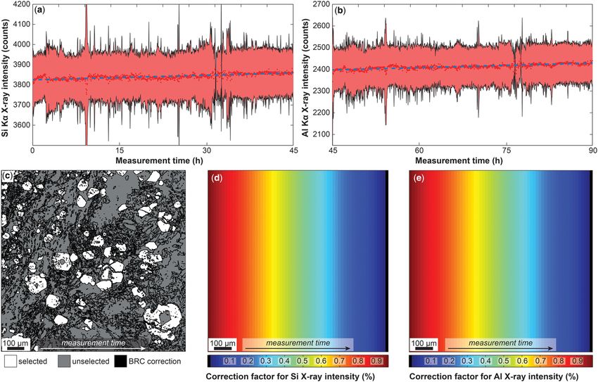
Downloaded from http://sp.lyellcollection.org/ by guest on April 9, 2019

40                                              P. LANARI ET AL.

generated from high-resolution backscatter electron        appeared as 2D quantitative images. More important
images (Willis et al. 2017).                               than the quantification of element distribution pat-
    This chapter has a two-fold goal. The first is to       terns in two dimensions was the resulting interpreta-
present a summary of the technical and computa-            tion that the equilibrium conditions (here pressure
tional advances made over the past half-century            and temperature) changed during garnet growth.
that have provided the foundation for the more recent      The first quantitative maps of trace element concen-
developments. This review is partly based on case          trations by EPMA (Spear & Kohn 1996; Cossio et al.
studies where quantitative compositional mapping           2002) and LA-ICP-MS (Raimondo et al. 2017) were
has provided considerable benefits in investigation         also acquired using garnet and then used to quantify
of specific rock-forming processes. Secondly, we            (Kohn & Spear 2000) and model (Lanari et al. 2017)
introduce an advanced standardization function that        the amount of garnet resorption during cooling and
implements a correction for the X-ray continuum            exhumation. Clearly, the contouring technique of
(background) attributable to the X-ray bremsstrah-         Tracy et al. (1976) was a major step forward in our
lung (literally ‘braking radiations’) effect. This         understanding of garnet zoning systematics by
standardization procedure is implemented into an           EPMA. However, it has remained time consuming
improved workflow for the computer software                 and limited to very low spatial resolution.
XMapTools (Lanari et al. 2014b, available via                  Instrumental and computational improvements
http://www.xmaptools.com).                                 in the early 1990s have paved the way for the direct
                                                           acquisition of digital intensity maps in which a semi-
                                                           quantitative microanalysis is carried out at every
Quantitative compositional mapping: a                      beam location in a digitally controlled scan pro-
historical perspective                                     ducing numerical X-ray matrices (Marinenko et al.
                                                           1989; Newbury et al. 1990a, b; Launeau et al.
Point-by-point investigation of a surface by analysis      1994). Traditionally the maps were acquired in elec-
of the characteristic X-ray emission was initiated by      tric beam-tracking mode with a moving beam on a
Castaing (1952) who built the first practical micro-        stationary sample. Focusing issues were successfully
beam instrument called an electron probe micro-            solved during the analysis or by applying post-
analyser. Only a few years’ later, this technique          processing corrections (Newbury et al. 1990b and
was expanded to acquire 2D qualitative images of           references therein). The development of a high-
element distribution using the ‘flying spot X-ray’          precision computer-controlled x–y–z stage with an
method (Cosslett & Duncumb 1956). This analogue            absolute accuracy 100 000 pixels (up to several millions). For each
Marinenko et al. 1989).                                    element, the X-ray map is a matrix made of X and
    An alternative strategy applied by Tracy et al.        Y points forming a grid of pixels. The matrices,
(1976) consisted of measuring several high-resolu-         between 8 and 20 depending on the number of ele-
tion spot analyses within individually zoned grains        ments, are organized along a third dimension. A
and then extracting contour maps of chemical               project file thus contains several millions of mea-
composition. For the first time, garnet compositional       surements and this extensive geochemical dataset
zoning – already recognized along 1D transects             needs to be carefully evaluated and investigated
(Atherton & Edmunds 1966; Hollister 1966) –                along several successive steps of data processing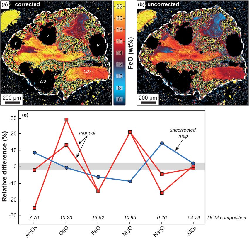
Downloaded from http://sp.lyellcollection.org/ by guest on April 9, 2019

                           QUANTITATIVE COMPOSITIONAL MAPPING BY EPMA                                         41

(see below). In the past, the multi-channel composi-      De Andrade et al. 2006). Acquisition times longer
tional classification could take a few hours for           than 30 h may involve a time-dependent drift in the
instance in the 1990s (Launeau et al. 1994), whereas      X-ray production caused by small variations of the
it is now generally performed within a few seconds        beam energy in the specimen. In this case, the result-
or minutes, using the automated clustering approach       ing drift needs to be corrected prior to standardiza-
implemented in the software XMapTools (Lanari             tion by flattening the intensity of a phase having a
et al. 2014b). The appearance of such user-friendly       homogeneous composition. Software tools for inten-
software solutions for classification and standardiza-     sity drift corrections are presented below.
tion has increased the popularity of this technique           For the current example, the X-ray maps were
(Cossio & Borghi 1998; Goncalves et al. 2005; Tink-       standardized using spot analyses as internal stan-
ham & Ghent 2005; Lanari et al. 2014b; Ortolano           dards (Fig. 1c) and the software XMapTools 2.4.1
et al. 2014) and fostered the development of thermo-      (Lanari et al. 2014b). The calibrated map contains
dynamic models based on local bulk compositions           312 000 pixels. After the exclusion of the ‘mixed’
(see Lanari & Engi 2017 for a review).                    pixels occurring at the grain boundaries, c. 290 000
                                                          spatially resolved fully quantitative analyses were
                                                          obtained. The average analytical precision for a
Precision and accuracy of quantitative                    single garnet pixel composition ranges between
compositional mapping by EPMA                             2.8% for Si and 20% for Mg (2σ, see Table 1).
                                                          One of the main advantages of the quantitative map-
Presented below is an example of quantitative map-        ping approach compared to traditional single-spot
ping by EPMA with a typical analytical setup, to          analyses is that the composition of several pixels of
show some advantages of this approach compared            homogenous material can be averaged, significantly
to single-spot analyses. A map of 600 × 520 pixels        increasing the analytical precision and the possibility
was generated at the Institute of Geological Sciences     to detect slight compositional zoning. An averaging
of the University of Bern using a JEOL 8200 superp-       over a 10 × 10 µm2 square window (as in the one
robe instrument, based on two passes (i.e. two map        plotted in Fig. 1a) reduces, for example, the mean
acquisitions). Accelerating voltage was fixed at           analytical uncertainty of garnet composition to
15 keV, specimen current at 100 nA, the beam and          0.28% for Si and 2% for Mg. Statistic tools are there-
step sizes at 1 µm and the dwell time at 160 ms.          fore needed to integrate pixel information along
This setup enabled measuring 9 elements by WDS            several spatial and compositional dimensions to
and 7 elements by EDS. The total measurement              identify and quantify small amounts of composi-
time for mapping was approximately 30 h corre-            tional zonation in the analysed sample (Cossio &
sponding to 15 h per scan (Fig. 1). Note that a shorter   Borghi 1998; Tinkham & Ghent 2005; Lanari et al.
dwell time may be used to save measurement time,          2014b). The example presented above shows that
but it affects the analytical precision proportionally    quantitative X-ray mapping represents an extremely
(see below). In this example, the total measurement       precise analytical technique, opening new prospects
time can be reduced to 15 h using a dwell time of         for accurate studies of various geological materials.
80 ms and 7.5 h using a dwell time of 40 ms.
    The investigated sample is a garnet-bearing meta-
sediment from Val Malone (Southern Sesia Zone,            Quantitative compositional mapping as a
Italian Western Alps) recording blueschist to             tool to track compositional changes and
eclogite-facies conditions during the Alpine Orog-
eny (Pognante 1989). To track possible drift in the       investigate rock-forming processes
X-ray production during the time window of the            In the past 15 years, the quantitative compositional
map acquisition, the average and standard deviation       mapping technique has been intensively applied to
(2σ) of the aluminium Kα X-ray counts of every sin-       metamorphic and magmatic rocks in order to inves-
gle line scan (corresponding to a single column in        tigate specific petrological processes. In the follow-
the image and an acquisition time of 90 s) in the         ing sections we provide a short review of a few
map were plotted against the measurement time             key studies that emphasize the advantages of this
(Fig. 1d). Aluminium is expected to be constant in        technique.
the alpine garnet in the absence of ferric iron
(labelled Grt2 in Fig. 1a). It is interesting to note
that no significant time-dependent intensity drift         Modal abundances and local bulk
was observed during this first pass and thus the cor-      compositions
responding X-ray maps can be directly transformed
into maps of element concentrations using one of          The quantitative mapping technique can be very
the standardization procedures available in the liter-    helpful in determining modal abundances of mineral
ature (e.g. Cossio & Borghi 1998; Clarke et al. 2001;     phases and thus the trace element distribution among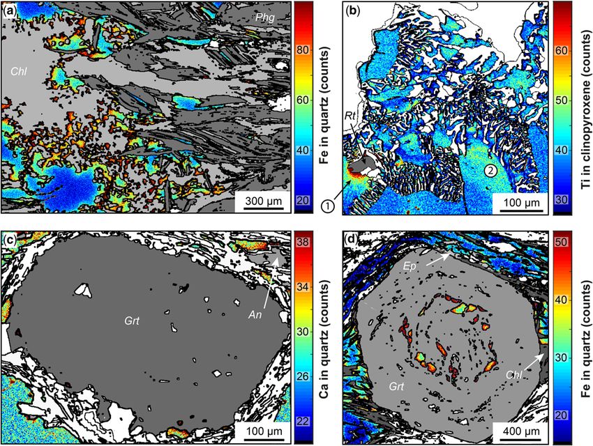
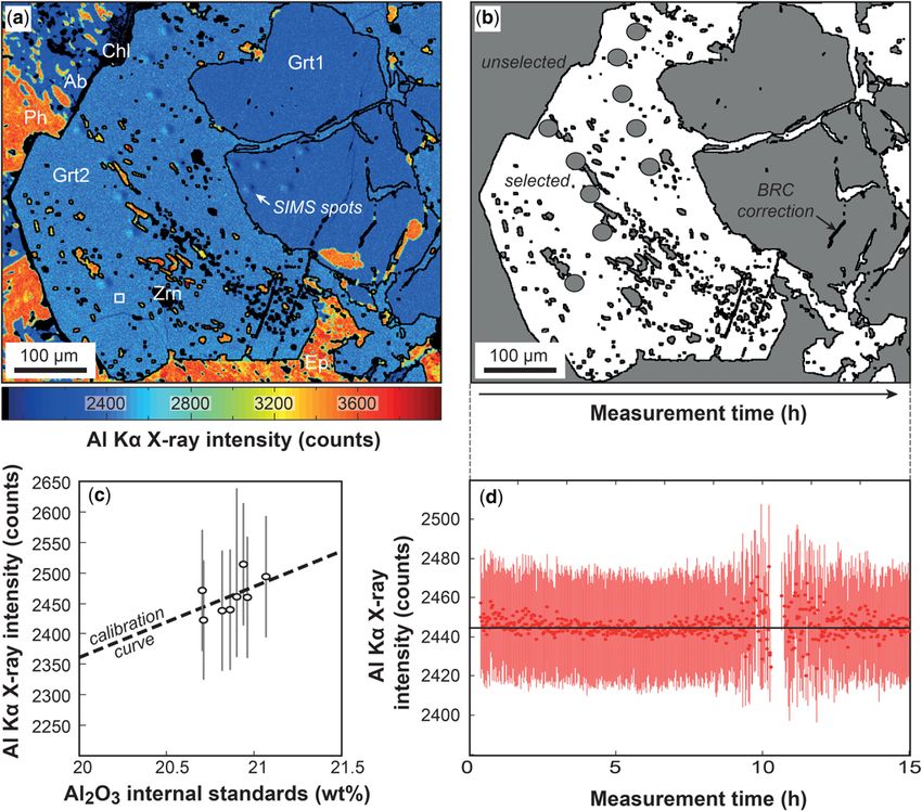
Downloaded from http://sp.lyellcollection.org/ by guest on April 9, 2019

42                                                P. LANARI ET AL.

Fig. 1. Mapping example of a HP mylonite from the Southern Sesia Zone (Western Alps, Italy) and stability test of
the mapping conditions in homogeneous material during analysis. (a) Semi-quantitative Al Kα X-ray map. White
square (bottom left part of the garnet): example of integration 10 × 10 pixels window (see Table 1 and text for
details). The Al content in garnet core (Grt1) is lower due to the presence of Fe3+ substituting with Al. (b) Mask
image of the mapped sample. White: pixels used for the stability test. The phase boundaries were removed using the
BRC correction of XMapTools to avoid mixed pixels and secondary fluorescence effects. Ion probe spot analyses
(SIMS spots in panel a) were manually removed as the topography of the crater affected the measured X-ray intensity
because of variable absorption thickness. (c) Calibration curve (dashed line) for garnet Grt2 using the advanced
standardization procedure described in this study. The error bars represent the uncertainty on individual pixel
composition determined from the counting statistics (at 2σ) using a Poisson law. (d) Test for time-dependent drift in
Al Kα X-ray intensity of Grt2 with time. Al is assumed to be constant in Grt2 in the absence of significant variations
of XFe3+ (
Downloaded from http://sp.lyellcollection.org/ by guest on April 9, 2019

                                QUANTITATIVE COMPOSITIONAL MAPPING BY EPMA                                                          43

Table 1. Uncertainties on raw map data acquired by EPMA

Element        Oxide          X-ray          1 pixel uncertainty             10 × 10 pixels                     20 × 20 pixels
               wt%†         intensity             (% 2σ)*                  uncertainty (% 2σ)*                uncertainty (% 2σ)*

Si             37.99           5040                 2.8172                         0.2817                           0.1409
Al             20.88           2370                 4.1082                         0.4108                           0.2054
Ca             12.23           3800                 3.2444                         0.3244                           0.1622
Fe             27.02           2950                 3.6823                         0.3682                           0.1841
Mg              0.99            100                20.0000                         2.0000                           1.0000
Mn              0.77            370                10.3975                         1.0398                           0.5199
Ti              0.10             30                36.5148                         3.6515                           1.8257

*The precision at 2σ-level (in %) was estimated on the average intensity of the garnet external rim pixels.
†
 Oxide wt% values are derived from quantitative spot analyses on the same garnet zone.

knowledge of the absolute concentrations of each                       required to obtain an accurate estimate of the local
pixel offers several additional advantages (see                        bulk composition (Lanari & Engi 2017). If the cor-
below).                                                                rection is not applied differences up to 5–10% are
    Samples with complex textures and heterogene-                      observed for Al2O3, FeO and MgO (Fig. 2). The
ities can be investigated locally, provided that quan-                 weight/pixel of FeO and MgO in pyroxene is higher
titative maps are available (Lanari et al. 2013;                       in the density-corrected map because the density
Carpenter et al. 2014; Riel & Lanari 2015). Ebel                       contribution of pyroxene to the average density of
et al. (2016), for instance, analysed both the size                    the domain is high (c. 110%). The weight/pixel of
and the distribution of chondrules and refractory                      Al2O3 in plagioclase is lower in the density-corrected
inclusions in chondrites. Because the maps were cal-                   map because plagioclase has a lower relative density
ibrated, they were able to extract the major element                   (c. 85%).
compositions of those objects. In another study,
quantitative maps were used to determine the bulk
composition of a single basaltic clast (with a size                    Thermobarometry from partially
of 1 × 1.2 mm2) in a lunar impact-melt breccia (Més-                   re-equilibrated minerals
zaros et al. 2016). Local bulk composition derived
from compositional maps has also been used for                         Partial re-equilibration in metamorphic rocks allows
mass balance computations in pseudomorphic reac-                       mineral relicts to be preserved through one or some-
tions (Centrella et al. 2015; Tedeschi et al. 2017)                    times more than one metamorphic cycles (Manzotti
and thermodynamic modelling of local equilibria                        & Ballèvre 2013). These relicts are important
(Marmo et al. 2002; Abu-Alam et al. 2014; Riel &                       archives for petrologists as they reflect changes in
Lanari 2015; Lanari & Engi 2017; Lanari et al.                         equilibrium conditions and can be used to retrieve
2017; Tedeschi et al. 2017; Centrella et al. 2018).                    individual pressure–temperature (P–T) stages or seg-
As noted by Lanari & Engi (2017), accurate determi-                    ments of the P–T paths. Single spot analyses by
nation of local bulk compositions requires a density                   EPMA are traditionally used to calculate activities of
correction in order to convert sampled area into                       end-members in solid solution and thus to model
weight fraction of a phase. Otherwise significant                       mineral reactions and mineral stability (see Spear
errors are introduced in the final local bulk composi-                  et al. 2017 for a review). Garnet is one of the most
tion, especially for elements sequestrated in dense                    famous thermobarometers and numerous calibra-
minerals. The example of Mészaros et al. (2016) is                     tions have been derived by the community to evalu-
used in the following to show how significant this                      ate the P–T conditions from garnet compositions
error can be. Uncorrected and corrected maps of                        either through the equilibrium with another Fe–Mg
FeO are shown in Figure 2 as well as the relative dif-                 phase or by using isochemical phase diagrams (Bax-
ference in the local bulk rock compositions estimated                  ter et al. 2017). However, one of the key aspects of
with several methods. Large discrepancies are                          garnet thermobarometry is an understanding of the
observed if the local bulk composition is approxi-                     processes that control the local mineral composition
mated using single spot analyses and modal abun-                       during growth (Kohn 2014). Compositional maps
dances obtained from semi-quantitative maps (red                       may help to clarify whether the observed composi-
curves in Fig. 2c). The discrepancy is smaller if                      tional zoning derives from continuous or discontinu-
quantitative maps are used since the compositional                     ous reactions involving equilibrium or transport-
variability of the mineral phases such as pyroxene                     controlled growth (Spear & Daniel 2001; Yang &
can be assessed. However, a density correction is                      Rivers 2001; Hirsch et al. 2003; Angiboust et al.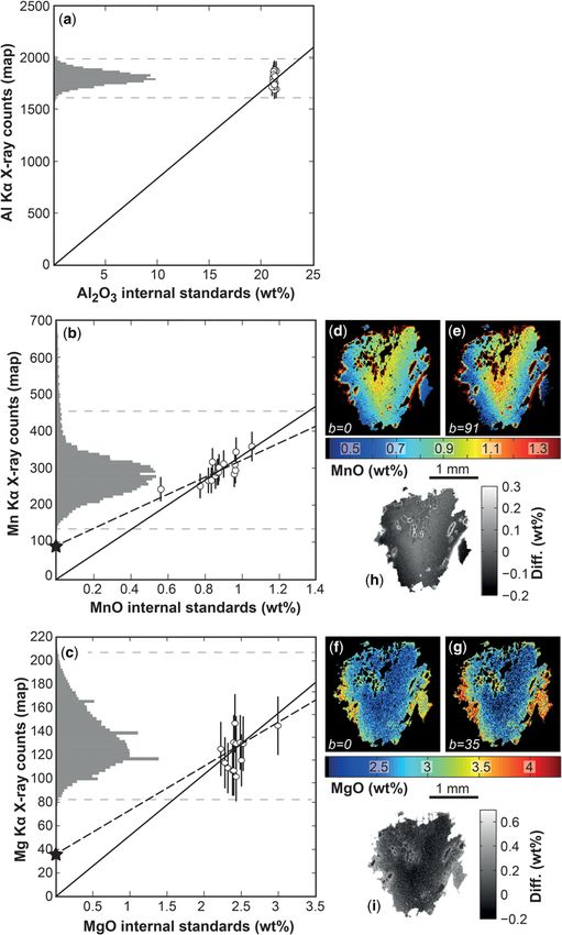
Downloaded from http://sp.lyellcollection.org/ by guest on April 9, 2019

44                                                P. LANARI ET AL.

Fig. 2. Local bulk composition of a single basaltic clast in a lunar impact-melt breccia (modified from Mészaros
et al. 2016) and comparison between density uncorrected and density corrected maps. (a) Density corrected map
(DCM) of FeO (in wt%); (b) density uncorrected map of FeO. Mineral abbreviations are from Whitney & Evans
(2010), v is vesicle. (c) Relative differences (in %) of the local bulk compositions obtained with several methods to a
reference composition obtained from the density corrected map using XMapTools. Density values of 2.33, 3.46 and
2.27 g cm−3 were used for cristobalite, pyroxene and plagioclase respectively. Method 1: manual – the compositions
were obtained from the modal abundances determined using semi-quantitative maps and the average composition of
spot analyses (shown in red, each curve representing a different set of spot analyses). Method 2: uncorrected map –
the composition is obtained from the density uncorrected map in XMapTools. The dashed lines show the domain that
was used to generate the local bulk compositions. The same domain was used to determine the modal abundances for
the manual method.

2014; Ague & Axler 2016; Lanari & Engi 2017).                 variability, not only through the mineral assemblage,
Empirical and semi-empirical thermometers and                 but also within a single grain has proven to be a great
barometers are also available for a large spectrum            assistance to thermobarometric studies (Marmo et al.
of magmatic and metamorphic mineral phases (for               2002; Lanari et al. 2013; Abu-Alam et al. 2014;
variable bulk rock compositions) and can be easily            Loury et al. 2016). More challenging are the high-
applied to derive temperature or pressure maps (De            variance assemblages involving phyllosilicates form-
Andrade et al. 2006; Lanari et al. 2014a, b; Trincal          ing at lower metamorphic conditions. Originally,
et al. 2015). The identification of the compositional          their investigation has required a multi-equilibrium
Downloaded from http://sp.lyellcollection.org/ by guest on April 9, 2019
QUANTITATIVE COMPOSITIONAL MAPPING BY EPMA 45
approach that relies on complex solid solution mod- a given range of composition or equilibrium condi-
els (Vidal & Parra 2000; Vidal et al. 2001, 2006; tions (Lanari et al. 2014b). The spatial distribution
Parra et al. 2002, 2005; Dubacq et al. 2010). These of the three groups of muscovite is shown in
techniques had significant successes when applied Figure 3f. Their relative distribution in both S1 and
to compositional maps as the P–T conditions of for- S2 cleavages can be quantified (Fig. 3e). These
mation can be put into a micro-textural context results are in line with those of Airaghi et al.
(Vidal et al. 2006; Ganne et al. 2012; Lanari et al. (2017a) showing that the metamorphic conditions
2014c; Trincal et al. 2015; Scheffer et al. 2016). It retrieved for the muscovite groups in different micro-
becomes therefore possible to apply multi-equilib- structural positions do not reflect the P–T conditions
rium thermobarometry to specific mineral phases of the microstructure-forming stages; rather they
that are observed in textural equilibrium. The assim- document successive fluid-assisted re-equilibration
ilation of the textural equilibrium to the thermody- events. Matrix minerals can continue to partially
namic equilibrium can lead to misinterpretation of re-equilibrate during prograde metamorphism once
the textural and compositional relationship (see the deformation ceased. Similar replacement textures
below). have also been documented in other phases such as
The investigations of the re-equilibration pro- chlorite (Lanari et al. 2012), biotite (Airaghi et al.
cesses in local mineral assemblage require a forward 2017a) and garnet (Martin et al. 2011; Lanari et al.
thermodynamic model (Lanari & Engi 2017). Yet 2017) using quantitative compositional mapping.
compositional maps have shown that the phyllosili-
cates in the mineral matrix of metapelite preferen-
Petrochronology
tially re-equilibrate in zones of high strain, while
they are preserved in zones of low strain such as The technique of quantitative compositional map-
microfold hinges (Abd Elmola et al. 2017; Airaghi ping is extremely helpful in petrochronological stud-
et al. 2017a, b). The compositional variability ies (see Engi et al. 2017) in linking metamorphic
observed within the different microstructural posi- stages and reactions to ages retrieved from major
tions and the quantification of the modal abundance and accessory minerals (Williams et al. 2017). In
of each compositional group have been used to dem- favourable cases, an age map can be constructed
onstrate that the phyllosilicates partially re-equili- and reveals the continuous spatial distribution of
brated during prograde metamorphism through ages (Goncalves et al. 2005). Otherwise, quantitative
pseudomorphic replacement. This process is mostly compositional mapping allows the most appropriate
controlled by the presence of a metamorphic fluid spots for dating to be identified. For example, quan-
in the intergranular medium. In a detailed study of titative compositional mapping of allanite may
muscovite composition in amphibolite-facies meta- reveal the existence of cores and rims of different
pelite, Airaghi et al. (2017a) retrieved the P–T con- composition that, if large enough, could be dated
ditions of different muscovite compositional groups separately (Burn 2016; Engi 2017). The mapping
observed in different microstructural domains. The of the compositional heterogeneities in white mica
example of Airaghi et al. (2017a) is used in the fol- can highlight the most homogeneous grains for the
lowing to show how detailed investigation can be 40Ar/39Ar dating. In addition, it provides a strong
carried out using the quantitative mapping approach. petrological basis for interpreting the variability
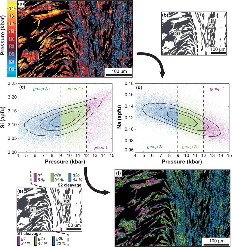
A pressure map (Fig. 3a) has been calculated from of in-situ 40Ar/39Ar dates (Airaghi et al. 2017b).
the compositional maps of muscovite at a fixed tem- The spatial resolution is often lower than the charac-
perature of 525°C using the method of Dubacq et al. teristic size of the compositional variations in mica
(2010) and the program ChlPhgEqui 1.5 (Lanari (Cossette et al. 2015; Berger et al. 2017; Laurent
2012). The pressure condition of each pixel is plotted 2017).
against P- and T-dependent elements such as Si To conclude this short overview, we can state
(Fig. 3c) and Na (Fig. 3d) in atom per formulae unit that quantitative mapping is therefore becoming an
(apfu). Muscovite was classified into three groups: essential tool to provide a comprehensive image of
the relicts of the HP stage (group 1 in Fig. 3), the the petrological, thermobarometric and geochrono-
phengite re-equilibrated between the pressure peak logical evolution of metamorphic rocks.
and the temperature peak (group 2a in Fig. 3), and
the muscovite re-equilibrated at the temperature
peak (group 2b in Fig. 3). The groups 2a and 2b cor- Standardization techniques: advantages
respond to the compositional group msB of Airaghi and pitfalls
et al. (2017a). Here the distinction is based on equi-
librium conditions rather than on compositional cri- The extraction of elemental concentration values
teria. The main advantage of using compositional from X-ray intensities requires matrix and other cor-
maps and chemical diagrams is the ability to depict rections. The X-ray data need to be standardized
the spatial distribution of any group of pixels within post-collection either relative to similar data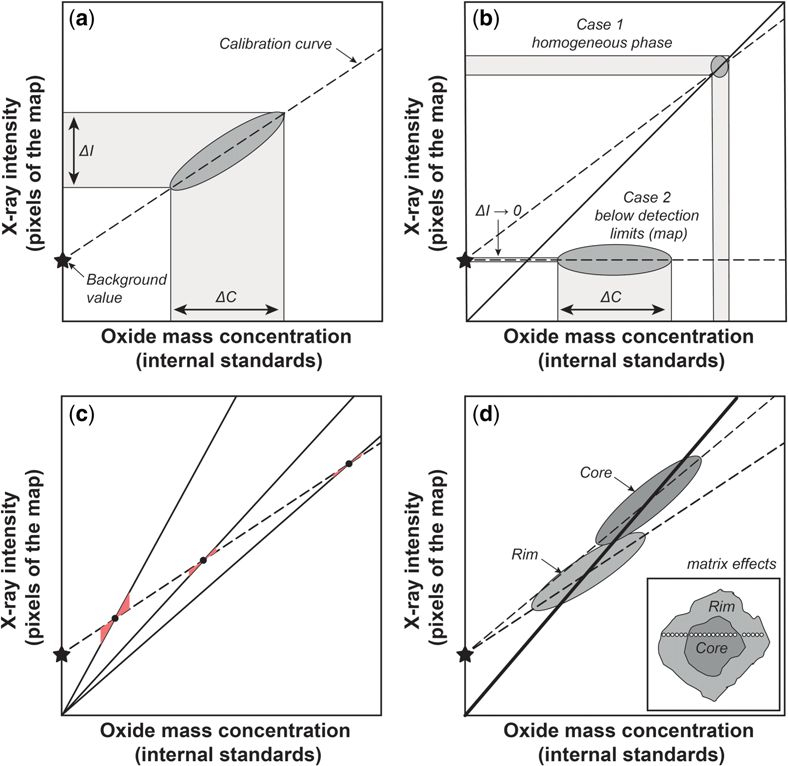
Downloaded from http://sp.lyellcollection.org/ by guest on April 9, 2019

46                                               P. LANARI ET AL.

Fig. 3. Pressure map and microstructural control on the degree of muscovite re-equilibration. (a) Pressure map of
sample to13-4 from Airaghi et al. (2017a) calculated using the calibration of Dubacq et al. (2010) at 525°C.
(b) Mineral sketch of the mapped area showing the microstructural domains associated to cleavage 1 (S1) and 2 (S2).
(c) Pressure v. Si (apfu) diagram. (d) Pressure v. Na (apfu) diagram. The three groups are based on the equilibrium
conditions obtained in (a). The group 1 contains all the muscovite pixels with pressure ranging between 15 and
12 kbar, the group 2a between 12 and 9 kbar and the group 2b between 9 and 4 kbar. (e) Mineral sketch of the
mapped area showing the fraction of each group in the two microstructural domains S1 and S2. (f ) Map showing the
spatial distribution of the pixels corresponding to each group.

collected on natural and synthetic standards using an       Castaing’s first approximation to quantitative
empirical correction scheme (Jansen & Slaughter             analysis and matrix effects
1982; Newbury et al. 1990a, b; Cossio & Borghi
1998; Clarke et al. 2001; Chouinard & Donovan               As first noted by Castaing (1952), the primary gener-
2015) or against internal standards assuming no             ated X-ray intensities are proportional to the respec-
matrix effects (De Andrade et al. 2006). Those tech-        tive weight concentration of the corresponding
niques are separately described in the following.           elements in the specimen. In the absence of
Downloaded from http://sp.lyellcollection.org/ by guest on April 9, 2019

                            QUANTITATIVE COMPOSITIONAL MAPPING BY EPMA                                         47

significant matrix differences between unknown                  Clarke et al. (2001) applied this procedure to
and standard materials, this assumption can be              standardize X-ray maps into a map of oxide mass
expressed as:                                               concentrations. Several tests have indeed shown
                                                            that the Bence & Albee (1968) procedure yields
                      Ciunk Iiunk                           results comparable to those obtained with the ZAF
                            ≈ std                    (1)    method (Goldstein et al. 2003) while reducing sig-
                      Cistd   Ii
                                                            nificantly the computation time for corrections
                                                            (Clarke et al. 2001). The accuracy of this method
where the terms Ciunk and Cistd are the composition         mostly depends on the quality of the α-factor esti-
expressed in weight concentration of the element i          mates, as well as the choice of homogeneous and
in the unknown and the standard and the terms Iiunk         well-characterized standard materials. Most of the
and Iistd represent the net corresponding X-ray intensi-    correction factors for oxides and silicates are well
ties corrected for continuum background (see below)         constrained and updates including small improve-
and any possible other issues such as peak overlap          ments are regularly published (Albee & Ray 1970;
or drift. In the case of significant physical and/or         Love & Scott 1978; Armstrong 1984; Kato 2005).
chemical differences between the unknown and the            The software XRMapAnal (Tinkham & Ghent
standard (i.e. matrix effects), equation (1) becomes:       2005) uses the Bence–Albee algorithm to standard-
                                                            ize X-ray maps and provides several tools to dis-
                     Ciunk     I unk                        play maps, compositional graphs and to perform
                       std
                           = ki istd                 (2)
                     Ci         Ii                          advanced statistical analyses.

where k represents a correction coefficient expressing
the non-linear matrix effects. In the specialized litera-
                                                            ZAF and ϕ(ρz) corrections
ture these effects are divided into atomic number (Zi),     The ZAF matrix correction was the first generalized
X-ray absorption (Ai) and X-ray fluorescence (Fi)            algebraic procedure. This standardization method is
effects. The correction must be applied separately          based on a more rigorous physical model taking
for each element present in both the analysed speci-        into account the atomic number effects, the absorp-
men and in a given standard reference material.             tion and fluorescence in the specimen. The ratio of
                                                            concentration in unknown and standard of an ele-
Bence–Albee empirical correction                            ment i is given by

The empirical procedure of Bence & Albee (1968) is                           Ciunk         I unk
based upon known binary experimental data and it                               std
                                                                                   = [ZAF]i istd              (5)
                                                                             Ci             Ii
involves less computation time than the ZAF correc-
tion described in the following. It assumes a simple
hyperbolic calibration curve between the weight             where [ZAF]i is the ZAF correction coefficient. Typ-
concentrations and the net intensities of a given           ical values of the ZAF coefficient for metals are
oxide in a binary system (Ziebold & Ogilvie 1964).          reported in several text books (e.g. Goldstein et al.
The calibration curve is described in terms of a single     2003; Reed 2005).
conversion parameter known as the α-factor                      The direct calculation of absorption in the origi-
                                                            nal ZAF correction scheme was lately improved by
               (1 − IA )       (1 − CA )                    introducing an empirical expression of ϕ(ρz) to cor-
                         = aAB                       (3)    rect for absorption (Packwood & Brown 1981). In
                  IA              CA                        the mid-1980s several ϕ(ρz) algorithms (e.g. Riveros
                                                            et al. 1992), including more accurate sets of mass
with αAB the α-factor for a binary between elements         absorption coefficients, were successively devel-
A and B; IA and Ca the net intensity and mass con-          oped: PROZA (Bastin et al. 1986), citiZAF (Arm-
centration, respectively. This approach has been            strong 1988), PAP (Pouchou & Pichoir 1991),
generalized by Bence & Albee (1968) to more com-            XPhi (Merlet 1994). Some of them are still used in
plicated oxide systems of n components using a              modern EPMA instruments. It is crucial for the
linear combination of α-factors such that:                  ZAF or ϕ(ρz) corrections to analyse all the major
                                                            and minor elements present in the specimen to ensure
         Cn k1 an1 + k2 an2 + · · · + kn ann                that all the possible matrix effects are taken into
            =                                        (4)
         In       k1 + k2 + · · · + kn                      account.
                                                                Both ZAF and ϕ(ρz) correction algorithms have
where αn1 is the α-factor for the n1 binary used to         been applied to X-ray maps in order to generate
determine the concentration of element n in a binary        maps of oxide mass concentrations (Jansen &
between n and 1.                                            Slaughter 1982; Cossio & Borghi 1998; Prêt et al.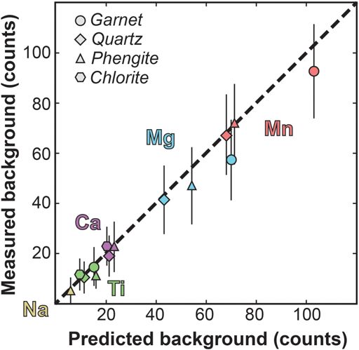
Downloaded from http://sp.lyellcollection.org/ by guest on April 9, 2019

48                                             P. LANARI ET AL.

2010) and this option is currently available in the       computer program (De Andrade et al. 2006), in the
software PetroMap (Cossio & Borghi 1998) and in           software solutions XMapTools (Lanari et al.
CAMECA’s commercial software provided with                2014b) and QntMap (Yasumoto et al. in press).
the SX100. There are two main limits of this tech-
nique. First, it is necessary to perform an accurate
background correction to the X-ray maps prior to          Spatial and chemical resolution and
standardization. This correction requires either the      possible issues
acquisition of upper and lower peak background
maps or the use of models to predict the theoretical      Spatial resolution
background values (e.g. Tinkham & Ghent 2005).
The MAN algorithm for instance allows the back-           In compositional mapping, the spatial resolution is
ground value to be predicted from the mean atomic         determined by the spacing of spot measurements
number of the specimen (Donovan & Tingle 2003;            and the X-ray excitation volume of the electron
Chouinard & Donovan 2015; Wark & Donovan                  beam. It is recommended to use a beam size smaller
2017), significantly reducing the total acquisition        than the pixel size to reduce overlapping (see XMap-
time. The second limitation is the large relative         Tools’ user guide for examples). For a given spacing
uncertainty in the intensity of each pixel (see           between two pixels, an increasing beam size will
Table 1). This uncertainty is propagated through          increase the fraction of ‘mixed’ pixels (i.e. mixed
the ZAF factors. To overcome this issue, Jansen &         phases see below).
Slaughter (1982) applied a preliminary ZAF correc-
tion to a group of pixels of the same mineral phase in    Chemical resolution
order to derive an estimate of the ZAF correction fac-
tors yielding for this phase. These factors are then      The chemical resolution of an individual pixel
used to correct compositionally similar pixels. This      depends on the dwell time, the accelerating voltage
option is not available to our knowledge in any com-      and the beam current. The relative precision of any
mercial software or freeware solution.                    measurement can be estimated using counting statis-
                                                          tics (the generation of characteristic X-rays is a Pois-
                                                          son process) from the total number of X-rays
Internal standardization using high-precision             collected by the detector. Examples of analytical pre-
spot analyses                                             cisions for different elements are given in Table 1.
                                                              As shown in the introduction, as soon as several
Of primary importance in routine EPMA analyses            pixels are taken into account, the relative uncertainty
are the analytical precision and accuracy of spot         and detection limits decrease relative to the values
analyses. The quality of standardization in spot anal-    obtained by single pixel counting statistics. Averag-
ysis can be quickly evaluated using either a reference    ing of pixels of unzoned material or of a single
material with known concentration, or stoichiomet-        growth zone virtually increases the counting time
ric constraints on unknown mineral phases. These          thus reducing the relative uncertainty (Table 1).
tests are routinely applied before each analytical ses-   This effect applies to any map, as the human eye is
sion and ensure the high quality of the data produced.    an outstanding integrator of visual information.
The internal standardization procedure of X-ray           The human brain is able to detect gradients even in
maps takes advantage of the excellent quality of spot     noisy signals. If a mineral phase extends over a sub-
analyses. The goal is to calibrate the X-ray maps of      stantial lateral range of pixels, it might be possible to
every mineral phase using high precision spot analy-      discern compositional zoning below the detection
ses of the same mineral phase (Mayr & Angeli 1985;        limit despite the noise that results from statistical
De Andrade et al. 2006). In this case, there are no       fluctuations in the count of a single pixel (Newbury
matrix effects between the unknowns (X-ray maps)          et al. 1990a; Friel & Lyman 2006).
and the standards (spot analyses):

                        Cistd unk∗                        Issues
              Ciunk =         I    + Iiback        (6)
                        Iistd i                           Radiation damage. Some elements, and particularly
                                                          light elements, are affected by degradation induced
with Iiunk∗ the X-ray intensity of the unknown uncor-     by local heating effects from electron beam exposure
rected for background and Iiback the intensity of back-   over time. Either an increase or decrease in intensity
ground. This approach results in a strong dependence      could be observed because of radiation damage. A
of the accuracy of the compositional maps upon the        decrease in intensity may reflect a loss of mass by
accuracy of the spot analyses selected for the stand-     volatilization. The low-energy X-rays of volatile ele-
ardization. The internal standardization procedure        ments undergo a strong self-absorption in the speci-
has been implemented in a MATLAB©-based                   men that increases if the beam energy is increased
Downloaded from http://sp.lyellcollection.org/ by guest on April 9, 2019
QUANTITATIVE COMPOSITIONAL MAPPING BY EPMA 49
(Goldstein et al. 2003). Therefore, light elements X-rays originate from different contributions. In
(Na. K, Ca) have to be measured with the lowest X-ray images, secondary fluorescence effects can
beam energy possible, during the first pass of the occur near phase boundaries (e.g. Fig. 4) or melt
beam over the mapped area. inclusions (Chouinard et al. 2014). Compositional
mapping is a powerful tool to detect potential
Secondary fluorescence effects. A secondary fluores- effects of secondary fluorescence that would not
cence effect occurs when the characteristic X-rays be seen otherwise. Figure 4 shows a few examples
of a given element generate a secondary generation involving an apparent compositional zoning that is
of characteristic X-ray of another element. Because caused by secondary fluorescence effects. Secondary
X-rays penetrate into matter farther than electrons, fluorescence can affect several elements and is
the interacting volume of X-ray-induced fluores- commonly associated with the presence of anorthite
cence is generally greater (up to 99% larger as (Ca), chlorite (Fe), epidote (Fe), garnet (Ca) or rutile
proposed by Goldstein et al. 2003). This volume (Ti). One of the best candidates in which to observe
may include more than one phase, and the induced secondary fluorescence effects is quartz (Fig. 4a, c, d).
Fig. 4. Examples of apparent compositional zoning in quartz caused by secondary fluorescence effects. The scale
bars show number of recorded X-ray counts. Mineral abbreviations are from Whitney & Evans (2010). Mixed pixels
have been removed using the BRC correction (see text). The phases shown in white do not play any role for
secondary fluorescence effects. (a) Map of a micaschist sample from the Briançonnais Zone (Chaberton area) in the
Western Alps (Verly 2014) showing the secondary fluorescence of Fe in quartz at the contact with chlorite (light
grey) but not with phengite (dark grey). White: plagioclase and rutile. (b) Map of a mafic eclogite from the Stak
massif in NW Himalaya (Lanari et al. 2013, 2014b). An apparent zoning in Ti is observed in clinopyroxene (area 1)
at the contact with rutile, caused by secondary fluorescence of Ti, while a ‘real’ compositional zoning of Ti is present
in clinopyroxene and correlated with the variations in other major element concentrations (area 2). White: garnet,
amphibole, plagioclase and Fe-oxide. (c) Map of a schist belonging to the TGU (Theodul Gletscher Unit) in the
Zermatt area. Secondary fluorescence of Ca observed in quartz at the contact with garnet (dark grey) and plagioclase
(light grey). White: rutile, titanite, apatite, phengite, paragonite, pyrite, zoisite and epidote. (d) Secondary
fluorescence of Fe in quartz at the contact with garnet (light grey) and chlorite (dark grey) in another schist from the
TGU. White: paragonite, phengite, albite, pyrite, chlorite, zoisite, rutile, titanite and apatite.Downloaded from http://sp.lyellcollection.org/ by guest on April 9, 2019 50 P. LANARI ET AL. The X-ray intensity caused by secondary fluores- WDS mapping with fixed stage and scanning cence in a surrounding mineral decreases from the beam, the beam may be scanned off the point of opti- source toward the inner part with a distance up to mum focus and the X-ray intensity decreases as a 100 µm at 15 keV, 100 nA and for counting time function of the deflection (Newbury et al. 1990b).
Downloaded from http://sp.lyellcollection.org/ by guest on April 9, 2019

                           QUANTITATIVE COMPOSITIONAL MAPPING BY EPMA                                          51

       recorded away from grain boundaries and             An advanced standardization procedure
       ‘mixed’ pixels recording mixing information         implemented in XMapTools’ workflow
       (Launeau et al. 1994). Only pure pixels can
       be used directly to measure the compositional       A description of the different steps of data processing
       variability of a given mineral phase. It is         is given in the following sections.
       important to minimize as much as possible
       the presence of mixed pixels in the maps by         Multi-channel compositional classification
       using small beam size (
Downloaded from http://sp.lyellcollection.org/ by guest on April 9, 2019
52 P. LANARI ET AL.
Sample surface topography. Sample topography, An example of time-dependent drift observed in a
such as holes or irregular surfaces, may have a signif- map acquired over c. 90 h is presented in Figure 5.
icant effect on the produced X-ray intensities. The The investigated sample is the same as the one
local topography introduces variable absorption described in the introduction (garnet-bearing metase-
path-length in different directions, so that the inten- diment from the Southern Sesia Zone in the Western
sity emitted varies according to the spectrometer Alps). The Si Kα X-ray map (measured during the
position (Newbury et al. 1990a). A TOPO map can first pass) and Al Kα X-ray map (measured during
be measured in JEOL EPMA instruments using the the second pass) of alpine garnet Grt2 were used to
solid-state BSE detector. This detector consists of track possible time-dependent drift and to define a
two opposite segments: one located at the top of correction function (Fig. 5). In this example, the
the image field and one located at the bottom. The observed time-dependent drift exhibits a constant
topographic image is constructed from the difference slope over the whole acquisition time corresponding
between the BSE signals returned by the two detec- to an average drift in the X-ray intensities of c. 0.02%
tors. The topography image corresponds to a light per hour (c. 1% for each scan of c. 45 h). The simi-
illumination at oblique incidence and suppresses larity of the drift in the two scans suggests that it
the atomic number contrast component of the BSE reflects a progressive defocusing of the beam caused
signal (Kässens & Reimer 1996). In the XMapTools by a slight inclination of the sample. This example
software, the topography correction can be applied shows that the beam stabilization system of the
using the TRC module (TRC is for TOPO-related JEOL 8200 superprobe used in this study performs
correction) when a correlation is observed between well compared to the probe current drift of 0.36%
the X-ray intensities of an element in a given phase per hour reported in Cossio & Borghi (1998). How-
and the intensity of the TOPO map. The magnitude ever, other maps have shown significant time-
of the correction depends on the spectrometer used, dependent drift caused by either vacuum failure in
the element and the mineral phase analysed as the the gun chamber or electron beam current drift. In
absorption changes with the position of the spec- this case it is vitally important to detect such a drift
trometer and the density of the target material. and to apply the appropriate correction to the X-ray
maps prior standardization.
Time-dependent drift. A time-dependent drift in
the X-ray production related to small variations in Mixed pixels and BRC correction. Mixed pixels are
the beam current at the specimen surface may be commonly observed at the boundary between two
observed for acquisition periods exceeding 24 h phases, depending on the map resolution and beam
(Fig. 5). There are three major causes for time- size (see XMapTools’ user guide for examples).
dependent drift of the X-ray intensities to occur. Resulting localized features do not represent authen-
First, the probe current can drift during the analysis tic mineral zoning. Mixed pixels can be filtered using
(e.g. Cossio & Borghi 1998). Secondly, the vacuum the border-removing correction (BRC) available in
conditions in the gun or the specimen chamber can XMapTools. This correction removes the pixels
change with time, causing more (or less) interactions located between the different masks of the selected
between the electron beam and the gas particles thus mask file. The correction may be applied for different
decreasing (or increasing) the specimen energy and sizes of the mixing zone depending on the map res-
the production rate of characteristic X-rays. For olution. An alternative strategy is to evaluate the pro-
instance, an abrupt increase of the pressure in the portion of phases in each mixed pixel using a
gun chamber may cause a sharp decrease in the mea- distribution-based cluster analysis (Yasumoto et al.
sured X-ray intensities. The third cause may be in press).
related to beam-defocusing issues during scanning
on a non-flat surface. Defocusing indeed affects the Position of maps and standards. Before performing
geometry and size of the interaction volume thus the analytical standardization, the position of the
affecting the specimen energy density where the maps and the spot analyses must be tested and, if
characteristic X-rays are produced. The resulting necessary, modified, based on statistical criteria. It
drift might be corrected prior to standardization is critical to guarantee that the positions of the spot
regardless of the cause of the variation as soon as analyses used as internal standard have not shifted,
the time-dependency can be retrieved. For the cor- i.e. that the analysed volume is the same in both anal-
rection to be performed, a phase equally distributed yses. In order to detect such a shift, the standard data
within the mapped area and showing a homogeneous (spot analyses, in wt%) can be compared with the
composition in a given element must be identified. intensity data (in counts) of the corresponding pixels
The Intensity Drift Correction (IDC) tool has been on the map, as shown in Figure 6. An algorithm that
implemented in XMapTools 2.4.1 for this purpose. detects the optimal position of the maps and the spot
It enables detection of time-dependent drifts and analyses is available in XMapTools. A map of the
applies any correction function defined by the user. correlation coefficients between the standard andDownloaded from http://sp.lyellcollection.org/ by guest on April 9, 2019
QUANTITATIVE COMPOSITIONAL MAPPING BY EPMA
Fig. 5. Example of time-dependent drift for a total measurement time of 90 hours on the sample described in Figure 1. (a, b) Evolution of Si Kα X-ray intensity and Al Kα
X-ray intensities in Grt2 with time. Red spots: mean values of each pixel column (corresponding to time interval of c. 160 seconds). Vertical bars: standard deviation (at 2σ). The
observed time-dependent drift is fitted using linear function (blue dashed line). It is interesting to note that the slope of this function remains constant during the whole acquisition
time (two passes). (c) Mask image of the mapped area showing in white the pixels used for the stability test. The phase boundaries were removed using the BRC correction.
53
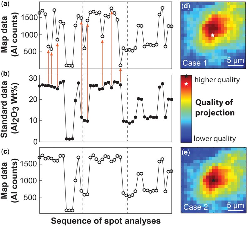
(d, e) Matrixes of correction factors (in %) used to correct the X-ray maps of Si Kα and Al Kα respectively. In both cases, the drift correction is lower than 1%.Downloaded from http://sp.lyellcollection.org/ by guest on April 9, 2019 54 P. LANARI ET AL. Fig. 6. Positions of spot analyses (internal standard) for the map shown in Figure 5 are tested and corrected using the SPC module of XMapTools. (a) Case 1: X-ray intensity signal of the Al Kα map pixels corresponding to the original position of the spot analyses obtained from the EPMA coordinates. (b) Al2O3 mass concentration of the spot analyses (internal standards). This trend is used as a reference to evaluate the quality of the projection. The red arrows mark the pixels showing a poor match with (a). (c) X-ray intensity signal of the Al Kα map pixels corresponding to the corrected position of the spot analyses. (d) Synthetic map of the quality of the projection for Case 1. The best position of the spot analyses (internal standard) on the map is calculated as described in the text. In this example, the correlation coefficients were calculated for a 21 × 21 pixels window centred on the original position (white star). The original position is shifted from the optimal position and may be corrected by moving the internal standard position on the map. (e) Synthetic map of the quality of the projection for Case 2. After the correction, the position (black star) corresponds with the best match. It is interesting to notice that even a shift of 2 µm can significantly affect the quality of the match and thus of the standardization. the intensity data for different X and Y positions is the quality of the projection by c. 20%), the standard calculated for each element. All maps are then com- position correction is crucial to obtain a reliable bined to produce a synthetic map evaluating the standardization overall quality of the projection. Examples of good and bad position of standards are shown in Figure 6. Advanced procedure for internal In the first case (Case 1 in Fig. 6a, d), the comparison standardization reveals a shift in the position of the spot analyses, corrected using the Standard Position Correction In the XMapTools software, analytical standardi- (SPC) tool by shifting vertically the positions of zation is performed using high-precision spot ana- the spot analyses by of 2 µm. In the second case, lyses as internal standards (Lanari et al. 2014b) to the quality of the projection was recalculated after obtain numerical concentrations. To be accurate, the correction (Fig. 6c, e). The match between standard X-ray maps need to be corrected for background (see values (in wt%, Fig. 6b) and the pixel intensity (in equation 6) prior to standardization. The background counts, Fig. 6c) is greatly improved. The projection correction is usually applied by using background in Case 2 plots in the optimal quality field of the values of the spot analyses (De Andrade et al. resulting synthetic map. Considering that a shift of 2006). However, it is not applicable if the map and few pixels can affect the quality of the match (i.e. spot analyses are acquired with different spectrome- in the example in Fig. 6, a shift of 2 µm decreases ter configurations. For high intensity:background
Downloaded from http://sp.lyellcollection.org/ by guest on April 9, 2019
QUANTITATIVE COMPOSITIONAL MAPPING BY EPMA 55
ratios, where Ii / Ii∗ − Ii . 20, the background cor- the standards (ΔC in Fig. 7a) to fit the slope of the
rection is not applied. The spot analyses are indeed calibration curve and to approximate the correspond-
already corrected for background and the map ing background (equation 6, see the star in Fig. 7a).
background effects on the calibration curve are For this approximation to be accurate, the spot anal-
negligible. On the contrary, for elements with low yses need to capture the majority of the composi-
intensity:background ratios, the background signifi- tional variability of the (zoned) minerals. This
cantly affects the slope of the calibration curve and pseudo-background correction is not applied to
a background correction is required (see below). homogeneous phases where ΔC is small (case 1 in
The acquisition of lower and upper background Fig. 7b). For trace elements, the compositional vari-
maps would triple the measurement time. Hence, ability can only be captured by the spot analyses
an advanced standardization and correction strategy (case 2 in Fig. 7d), showing that the measured ele-
has been implemented to overcome this problem and ment is below the detection limit for the mapping
is described in the following. This calibration does conditions (Lanari et al. 2014b). As previously men-
not require any background measurements and is tioned, the difference between a calibration using a
thus extremely powerful at low count rates where background correction and a calibration assuming a
the background correction is critical and not always fixed background value of zero decreases with
accurately predicted by MAN models (see Fig. 1 in increasing intensity:background ratios (Fig 7c). It
Wark & Donovan 2017). is also important to notice that this advanced tech-
The advanced standardization technique imple- nique can only be applied in absence of significant
mented in XMapTools 2.4.1 uses the variability matrix effects in the mineral phase. Matrix effects
commonly observed in the mass concentrations of generally occur if a strong compositional zoning is
Fig. 7. Advanced standardization technique based on internal standards. (a) The calibration curve for a given element
in a mineral phase is defined using the ranges in oxide mass concentration (ΔC) and in the X-ray intensity (ΔI). The
intercept values define the background correction to be applied to the phase of interest. (b) Internal standardization of
homogeneous phase (case 1) or of an element below the detection limit in mapping conditions (case 2). (c) Evolution
of the difference between standardizations with and without background correction with the oxide mass concentration.
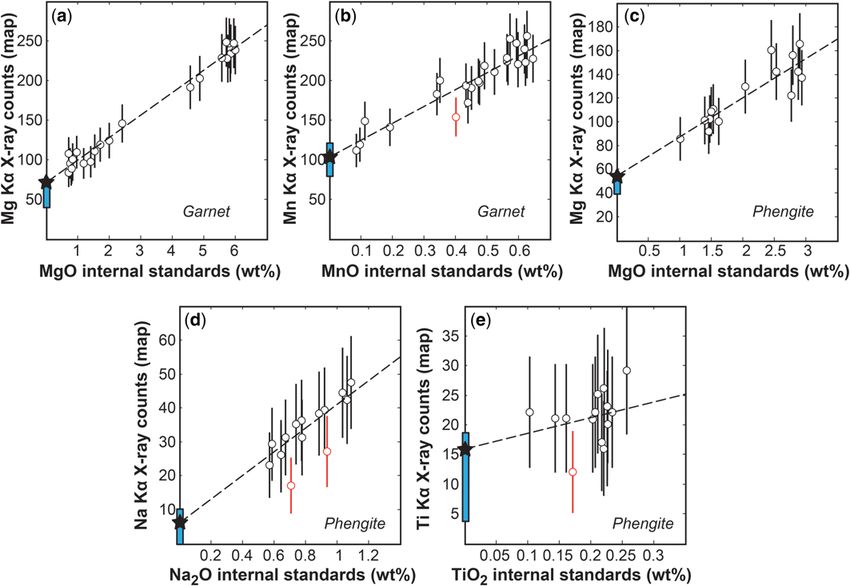
(d) Matrix effects in a single mineral (here garnet) causing changes in the slope of the calibration curve.Downloaded from http://sp.lyellcollection.org/ by guest on April 9, 2019 56 P. LANARI ET AL. Fig. 8. Example of standardization of garnet for Al, Mn and Mg. (a–c) Compositional diagrams showing the compositional ranges observed in the garnet pixels of the X-ray maps (histograms), the internal standards (white dots) with 2σ uncertainty and the calibration curves. The continuous lines are the calibration curves assuming no background, the dashed lines are the calibration curves of the advanced standardization method involving a pseudo-background correction. (d–g) Calibrated maps of MnO and MgO without background correction (d, f) and with background correction (e, g). The colour scale is identical for both images of the same element. (h, i) Difference maps in weight percentage.
Downloaded from http://sp.lyellcollection.org/ by guest on April 9, 2019

                           QUANTITATIVE COMPOSITIONAL MAPPING BY EPMA                                         57

observed between the core and the rim of a dense          observed compositional variability in Mn and Mg.
mineral such as garnet. In this case, it may be neces-    The absence of background correction (continuous
sary to apply several distinct standardizations one for   lines in Fig. 8b, c) significantly affects the standard-
each garnet composition (Fig. 7d). The matrix differ-     ized maps with relative differences up to 17% in
ences affect the slopes of the calibration curves (e.g.   MnO and 27% in MgO (Fig. 8d–g).
Lanari et al. 2014b) by underestimating the back-             To evaluate the reliability of this advanced stand-
ground value (see the continuous line in Fig. 7d).        ardization technique and especially the validity of
    An example of garnet standardization is given in      the background predictions, a phengite, chlorite
Figure 8. The investigated sample is a garnet-,           garnet-bearing metasediment from the Zermatt-Saas
kyanite- and staurolite-bearing metasediment from         Zone has been compositionally mapped at the Insti-
the Central Alps (Todd & Engi 1997). A millimetre-        tute of Geological Sciences of the University of Bern
sized garnet crystal has been compositionally             using a JEOL 8200 superprobe instrument with six
mapped at the Institute of Geological Sciences of         separate acquisitions of the same map area, two for
the University of Bern using a JEOL 8200 superp-          the peak measurements and four for the off-peak
robe instrument. Accelerating voltage was fixed at         background measurements. Background maps have
15 keV, specimen current at 100 nA, the beam and          been calculated assuming a linear background distri-
step sizes at 6 µm and the dwell time at 100 ms.          bution between the lower and upper background val-
The compositions of garnet core (MnO > 1 wt%)             ues. The measured background values have been
and rims (MnO < 0.7 wt%) are reported in Table 2.         compared with the predicted ones for garnet (Mg,
The standardization of aluminium does not require         Mn, see Fig. 9a, b) and phengite (Mg, Na, Ti see
any background correction (Fig. 8a), as the inten-        Fig. 9c–e). The predicted and measured background
sity:background ratio is typically higher than 60 for     values are in line within 2σ uncertainty for all the
almandine-rich garnet. The intensity:background           elements above detection limits for the mapping
ratios are much smaller for Mn and Mg (c. 3 for           conditions and with low intensity:background ratios
both cases) and thus a background correction is           (see Fig. 10). The measured background values for
required. For both elements the background values         Mn, Mg, Ca and Ti were also compared with the
have been approximated using the technique pre-           X-ray intensities measured in quartz. This test
sented above (see results in Fig. 8b, c). In this exam-   shows that the background maps were correctly mea-
ple the spot analyses captured a large range of the       sured off-peak and that the background values reflect
                                                          only the contribution of the X-ray bremsstrahlung.
Table 2. Average compositions and standard                To conclude, the advanced standardization tech-
deviation of garnet                                       nique provided in XMapTools can successfully cor-
                                                          rect the X-ray maps for background during the
              Garnet core              Garnet rim         standardization.
               (n = 825)               (n = 1282)

…          Average        SD       Average        SD      Local bulk compositions, structural formulas
                                                          and P–T maps
SiO2        37.54       1.092       37.804       1.061
TiO2         0.076      0.056        0.07        0.052    The standardized maps can be either merged to gen-
Al2O3       20.751      0.736       21.022       0.736    erate mass concentration images and extract local
FeO         32.78       1.076       31.823       1.062    bulk compositions (Lanari & Engi 2017) or treated
Fe2O3        0          0            0           0
                                                          separately to compute maps of elemental distribu-
MnO          1.11       0.095        0.59        0.083
MgO          2.107      0.292        2.873       0.344    tions in number of atoms per formula units or maps
CaO          4.917      0.264        5.086       0.283    of P–T conditions (De Andrade et al. 2006; Vidal
Na2O         0.035      0.047        0.036       0.05     et al. 2006; Lanari et al. 2014b).
K2O          0.052      0.032        0.055       0.05
Structural formula (12 anhydrous oxygen basis)
Si            3.031     0.055       3.03         0.054    Standards for data reporting
Al            1.975     0.062       1.986        0.062
Mg            0.254     0.035       0.343        0.041    A sufficient amount of information must be included
Fe2+          2.215     0.071       2.135        0.069    in publications (1) to enable the independent replica-
Mn            0.005     0.007       0.006        0.008    tion of the analytical measurements, and (2) to dem-
Ca            0.426     0.023       0.437        0.025    onstrate the validity of the proposed interpretations,
XAlm          0.746     0.012       0.722        0.014    including the uncertainty estimates (Potts 2012).
XSps          0.026     0.002       0.014        0.002
XPrp          0.085     0.011       0.116        0.013    As already proposed by Horstwood et al. (2016)
XGrs          0.143     0.008       0.148        0.008    for LA-ICP-MS U–(Th–)Pb data, comprehensive
                                                          details about both data acquisition and data
You can also read