Hillslope and groundwater contributions to streamflow in a Rocky Mountain watershed underlain by glacial till and fractured sedimentary bedrock - HESS
←
→
Page content transcription
If your browser does not render page correctly, please read the page content below
Hydrol. Earth Syst. Sci., 25, 237–255, 2021
https://doi.org/10.5194/hess-25-237-2021
© Author(s) 2021. This work is distributed under
the Creative Commons Attribution 4.0 License.

Hillslope and groundwater contributions to streamflow
in a Rocky Mountain watershed underlain by glacial
till and fractured sedimentary bedrock
Sheena A. Spencer1 , Axel E. Anderson1,2 , Uldis Silins1 , and Adrian L. Collins3
1 Department  of Renewable Resources, University of Alberta, Edmonton, T6G 2G7, Canada
2 Alberta Agriculture and Forestry, Government of Alberta, Edmonton, T5K 1E4, Canada
3 Sustainable Agriculture Sciences, Rothamsted Research, North Wyke, Okehampton, EX20 2SB, United Kingdom

Correspondence: Sheena A. Spencer (sheena.spencer@ualberta.ca)

Received: 2 March 2020 – Discussion started: 16 March 2020
Revised: 26 August 2020 – Accepted: 25 November 2020 – Published: 15 January 2021

Abstract. Permeable sedimentary bedrock overlain by                boundary of the measured sources in September and October.
glacial till leads to large storage capacities and complex sub-    The chemical composition of groundwater seeps followed
surface flow pathways in the Canadian Rocky Mountain re-           the same temporal trend as stream water, but the consistently
gion. While some inferences on the storage and release of          cold temperatures of the seeps suggested deep groundwater
water can be drawn from conceptualizations of runoff gen-          was likely the source of this late fall streamflow. Tempera-
eration (e.g., runoff thresholds and hydrologic connectivity)      ture and chemical signatures of groundwater seeps also sug-
in physically similar watersheds, relatively little research has   gest highly complex subsurface flow pathways. The insights
been conducted in snow-dominated watersheds with multi-            gained from this research help improve our understanding of
layered permeable substrates that are characteristic of the        the processes by which water is stored and released from wa-
Canadian Rocky Mountains. Stream water and source wa-              tersheds with multilayered subsurface structures.
ter (rain, snowmelt, soil water, hillslope groundwater, till
groundwater, and bedrock groundwater) were sampled in
four sub-watersheds (Star West Lower, Star West Upper, Star
East Lower, and Star East Upper) in Star Creek, SW Alberta,        1   Introduction
to characterize the spatial and temporal variation in source
water contributions to streamflow in upper and lower reaches       Forest disturbance from wildfire, pathogens, or forest har-
of this watershed. Principal component analysis was used to        vesting removes the forest canopy, increasing the total pre-
determine the relative dominance and timing of source wa-          cipitation that reaches the forest floor (Williams et al., 2019;
ter contributions to streamflow over the 2014 and 2015 hy-         Burles and Boon, 2011; Boon, 2012; Pugh and Small, 2012;
drologic seasons. An initial displacement of water stored in       Varhola et al., 2010), often altering the dominant flow path-
the hillslope over winter (reacted water rather than unreacted     ways, increasing streamflow quantity, and changing the tim-
snowmelt and rainfall) occurred at the onset of snowmelt be-       ing of flows in forested watersheds (Stednick, 1996; Scott,
fore stream discharge responded significantly. This was fol-       1993; Bearup et al., 2014; Winkler et al., 2017). However,
lowed by a dilution effect as snowmelt saturated the land-         large variability has been observed in streamflow responses
scape, recharged groundwater, and connected the hillslopes         following disturbance due to differences in disturbance type,
to the stream. Fall baseflows were dominated by either ri-         vegetation type, precipitation regimes, and soil moisture stor-
parian water or hillslope groundwater in Star West. Con-           age (Brown et al., 2005; Stednick, 1996). Some studies in Al-
versely, in Star East, the composition of stream water was         berta’s Rocky Mountains have reported little, if any, change
similar to hillslope water in August but plotted outside the       in streamflow following disturbance (Williams et al., 2015;
                                                                   Harder et al., 2015; Goodbrand and Anderson, 2016; An-

Published by Copernicus Publications on behalf of the European Geosciences Union.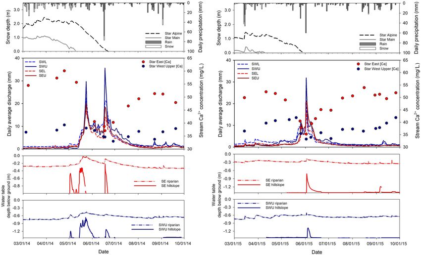
238        S. A. Spencer et al.: Hillslope and groundwater contributions to streamflow in a Rocky Mountain watershed

dres et al., 1987), but the mechanisms and watershed features          While these studies illustrate the influence of permeable or
(e.g., bedrock, surficial geology, and wetlands) potentially re-   fractured bedrock, deep soils, or till on baseflows, few stud-
sponsible for the lack of flow response have received little       ies have explored the combination of these storage zones on
attention. It has been suggested that watersheds exhibiting a      streamflow contributions (Burns et al., 1998; Dalke et al.,
lack of change in streamflow following disturbance might be        2012; Shaman et al., 2004). Burns et al. (1998) character-
associated with a large storage capacity and complex subsur-       ized the difference in deep (bedrock) and shallow (soils and
face flow pathways (Harder et al., 2015), but the higher-order     till) flow systems in the Catskill Mountains in New York,
controls regulating these muted responses remain unclear.          a region with both glacial till and permeable sedimentary
   Runoff generation has been extensively studied in regions       bedrock. Baseflow was maintained by discharge from peren-
with relatively impermeable bedrock overlain by shallower          nial springs which originated from bedrock fractures, rather
soils, which has led to broadly accepted conceptualizations        than contributions from the soil and till flow system (Burns et
of runoff dynamics (e.g., old water contributions to stream-       al., 1998). Conversely, fragipan layers contributed to differ-
flow, macropore flow, and subsurface streamflow generation         ing flow systems under dry vs. wet antecedent conditions in
– McGlynn et al., 2002; fill and spill hypothesis – Tromp-         central New York (state), USA (Dalke et al., 2012). Storm
van Meerveld and McDonnell, 2006; hillslope–stream con-            flow was generated from deep flow pathways below the
nectivity – Jencso et al., 2009). However, these conceptual-       fragipan during dry conditions and near surface flow path-
izations may not apply to regions with more complex struc-         ways during wet conditions. Comparatively little research
tural controls on runoff such as permeable bedrock, deeper         on runoff generation processes has been conducted in the
soils, or where multiple subsurface systems interact. Runoff       Canadian Rocky Mountains, in part due to deep snow that
generation in Alberta’s Rocky Mountains has added com-             is present for much of the year (October–May). While some
plexity because of the combination of both permeable sed-          studies have shown the importance of groundwater contribu-
imentary bedrock (highly fractured and faulted) and an over-       tions to streamflow in alpine watersheds in the Rocky Moun-
lying layer of deep, heterogenous glacial till (3 m deep, on       tains (Hood and Hayashi, 2015; McClymont et al., 2010),
average, and up to 10 m deep; AGS, 2004; Waterline Re-             the additional complexity imposed by highly heterogeneous
sources Inc., 2013). This is in contrast to regions such as the    glacial till and permeable bedrock in sub-alpine and upper
southern Rocky Mountains in Colorado (Sueker et al., 2000;         montane watersheds has limited more extensive research on
Cowie et al., 2017) and Montana (Jencso et al., 2009, 2010;        runoff dynamics of this region. As a first attempt to con-
Nippgen et al., 2015) that are often dominated by less per-        ceptualize runoff generation in Alberta’s Rocky Mountains,
meable metamorphic or igneous bedrock and thinner soils.           Spencer et al. (2019) quantified storage and precipitation–
While runoff generation processes may differ from these re-        runoff relationships from hydrometric data. Results indi-
gions, some inferences can be drawn from studies in regions        cated that runoff generation was strongly governed by the
with either permeable bedrock or deep soils alone. Water-          interaction of two zones of storage – soil and till storage
sheds with high bedrock permeability have been associated          and bedrock storage. The alpine region and sub-alpine/upper
with longer subsurface flow pathways and the slow release of       montane region were also identified as two separate hydro-
stored water to streams during baseflow (Uchida et al., 2006;      logic response units that differed in timing and flow pathways
Liu et al., 2004; Pfister et al., 2017). Uchida et al. (2006)      for runoff response. While Spencer et al. (2019) developed a
reported that a watershed with greater bedrock permeabil-          conceptualization of runoff generation for this region, they
ity had larger aquifer storage, and the subsequent release of      concluded that coupled flow and tracer approaches would be
stored water maintained baseflow later in the year. Similarly,     needed to reduce uncertainty in estimated flow contributions
Liu et al. (2004) showed that the recession limb of the annual     from each storage zone.
hydrograph in the Colorado front range Rocky Mountains                 Chemical signatures of source water (rain, snowmelt, soil
was driven by baseflow released from fractured bedrock, but        water, hillslope groundwater, till groundwater, and bedrock
Cowie et al. (2017) also stressed the importance of talus          groundwater) and stream water can be used to determine
slopes as a source of streamflow in the same alpine water-         which sources are contributing to streamflow during different
shed. Deep soils and till deposits with large storage capacities   flow conditions using end-member mixing analysis (EMMA;
have also been shown to sustain baseflows during drier peri-       Christophersen and Hooper, 1992). The key assumptions for
ods (Floriancic et al., 2018; Shanley et al., 2015). Deep sedi-    EMMA are that (1) the tracers are conservative, (2) the mix-
ment deposits in the Poschiavino watershed, in Switzerland,        ing process is linear, (3) source chemistry does not change
were associated with greater storage capacity and higher win-      temporally or spatially over the period or area studied (In-
ter baseflows compared to watersheds with shallow sediment         amdar, 2011; Hooper, 2003), and (4) all sources have been
deposits (Floriancic et al., 2018). Similarly, deep basal till     identified and have the potential to contribute to streamflow.
in the Sleepers River watershed in Vermont was associated          Many studies have used EMMA to conceptualize when dif-
with large storage capacity and low permeability that pro-         ferent geologic components are contributing to the stream
moted the extended maintenance of baseflow (Shanley et al.,        (e.g., James and Roulet, 2006; Cowie et al., 2017; Ali et
2015).                                                             al., 2010). However, this approach has been most successful

Hydrol. Earth Syst. Sci., 25, 237–255, 2021                                          https://doi.org/10.5194/hess-25-237-2021
S. A. Spencer et al.: Hillslope and groundwater contributions to streamflow in a Rocky Mountain watershed                      239

in smaller watersheds (1 km2 ) because of more constrained           ages) and exposed bedrock form the upper portion of alpine
variation in source water at smaller spatial scales (Hoeg et         zones in both sub-watersheds (Figs. 1 and 2). Talus slopes
al., 2000). Large watersheds could be characterized based on         terminate in the alpine and transitional forested regions of
smaller sub-watersheds (James and Roulet, 2006) if the sub-          the watershed, but streams or tributary features flowing from
watersheds are homogeneous. Others have concluded that               talus slopes have not been observed. There is also no evi-
where source water displays large variation or assumptions           dence of permafrost, ice lenses, or rock glaciers, unlike in
cannot be met, runoff processes should be described qualita-         other Rocky Mountain regions (Cowie et al., 2017; Clow
tively (Inamdar et al., 2013; Hoeg et al., 2000; Correa et al.,      et al., 2003; Hood and Hayashi, 2015; McClymont et al.,
2019).                                                               2010). Star West has a larger alpine region, with cirque till
   To expand on recent work carried out in the same study            deposits (estimated area of 0.14 km2 ; AGS, 2004), that in-
area by Spencer et al. (2019), this study aims to advance            cludes a narrow marshy area proximal to the stream that
the conceptualization of runoff generation in the Rocky              holds water throughout the summer and drains into the main
Mountains in Alberta, Canada. The objectives of this study           channel that is primarily bedrock in the upper reaches. The
were to (1) characterize how sources of stream water (rain,          Star East alpine region is smaller and more constricted than
snowmelt, soil water, hillslope groundwater, till groundwa-          in Star West (Fig. 2) and is comprised mostly of a grassy
ter, and bedrock groundwater) vary spatially, across four sub-       meadow, with the stream originating from springs where the
watersheds of a Rocky Mountain watershed, and temporally,            water table reaches the soil surface and is incised in collu-
from spring snowmelt to the start of the next year’s snow            vium with large boulders. In the lower reaches, streams in
accumulation period, and (2) determine the relative contri-          both sub-watersheds are composed of a series of step pools
butions of source water to the stream from spring to fall            incised in alluvium and colluvium, with some areas of ex-
for each sub-watershed. This study should help inform the            posed bedrock.
current conceptualization of runoff generation in northern              Two historical streamflow gauging sites exist in each sub-
Rocky Mountain watersheds.                                           watershed – a lower site (Star West Lower – SWL; Star
                                                                     East Lower – SEL) near the confluence of the two sub-
                                                                     watersheds (1540 m a.s.l.) and an upper site (Star West Upper
2   Study site                                                       – SWU; Star East Upper – SEU) located at approximately
                                                                     1690 m a.s.l. in the sub-alpine transition zone (Fig. 1). The
Star Creek watershed (10.4 km2 ; Fig. 1) is located in the east-     sub-alpine and upper montane zones are dominated by sub-
ern slopes of Canada’s Rocky Mountains, a region with frac-          alpine fir (Abies lasiocarpa) and Engelmann spruce (Picea
tured sedimentary bedrock overlain by glacial till. Average          engelmannii) above forests dominated by lodgepole pine
annual precipitation was 720 mm at Star Main (1482 m above           (Pinus contorta) at lower elevations (Dixon et al., 2014;
sea level – a.s.l.) and 990 mm at Star Alpine (1732 m a.s.l.;        Silins et al., 2009). Vegetation in upper and lower watersheds
Spencer et al., 2019). The area-weighted average annual              (Fig. 1) are distinguished by a transition between higher-
precipitation (2005–2018) was 950 mm, using the Thiessen             elevation alpine heath/shrub vegetation and sub-alpine fir-
polygon method and nine precipitation gauges at a range of           dominated forests in the upper watersheds and lodgepole-
elevations in and surrounding Star Creek; 50 %–60 % of the           pine-dominated forest in the lower watersheds.
precipitation falls in the form of snow (Spencer et al., 2019).
Soils are Eutric Brunisols (Canadian System of Soil Clas-
sification; also known as Eutric Cambisols in the Food and           3     Methods
Agriculture Organization system) approximately 1 m deep,
on average. Star Creek is underlain by unsorted and uncom-           3.1    Stream water chemistry
pacted glacial till, which is generally less than 3 m deep with
an estimated total area of 2.4 km2 (AGS, 2004; Fig. 1). Some         Stream water samples were collected from the four stream-
clay-rich till layers, likely from localized glacial ice melt fea-   flow gauging stations (SEL, SEU, SWL, and SWU; Fig. 1)
tures, occur intermittently throughout the watershed, result-        every 2 weeks, from April to October in 2014 and 2015,
ing in heterogeneous and uneven distribution of glacial till         to capture the full range of streamflow chemistry over the
throughout the watershed. Sedimentary geologic formations            hydrologically active period. Plastic bottles of 1 L in vol-
(Upper Paleozoic formation, Belly River–St. Mary Succes-             ume were triple rinsed prior to sample collection. Samples
sion, and Alberta Group formation) are primarily composed            were analyzed for major cations and anions (Na+ , Mg2+ ,
of shale and sandstone (AGS, 2004) and are highly fractured          Ca2+ , K+ , Cl− , and SO2−4 ) and silica (Si as SiO2 ) in the
due to folding and faulting (Waterline Resources Inc., 2013).        Biogeochemical Analytical Service Laboratory (University
   Star Creek includes two main sub-watersheds, namely Star          of Alberta). An inductively coupled plasma–optical emis-
East (3.9 km2 ; 1537–2628 m a.s.l.) and Star West (4.6 km2 ;         sion spectrometer (iCAP 6300; Thermo Fisher Scientific)
1540–2516 m a.s.l.). Unvegetated talus slopes (0.50 km2 in           was used to measure Na+ , Mg2+ , Ca2+ , and K+ with an an-
Star East and 0.53 km2 in Star West, digitized from orthoim-         alytical precision of 1.9 %, 3.0 %, 1.9 %, and 2.4 %, respec-

https://doi.org/10.5194/hess-25-237-2021                                             Hydrol. Earth Syst. Sci., 25, 237–255, 2021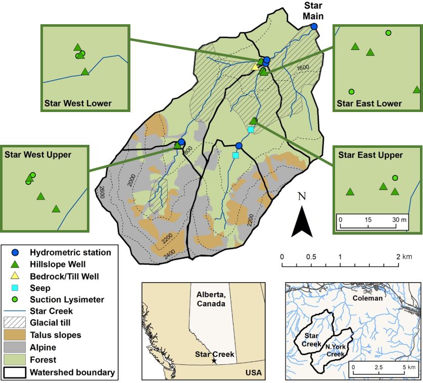
240 S. A. Spencer et al.: Hillslope and groundwater contributions to streamflow in a Rocky Mountain watershed
Figure 1. Star Creek watershed. Suction lysimeter and hillslope groundwater well locations are magnified in green boxes.
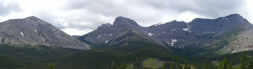
Figure 2. Star East (left) and Star West (right) sub-watersheds. The Star East alpine area is more constrained and smaller than the Star West
alpine area. Both sub-watersheds have steep headwalls with talus slopes in the alpine zone.
tively. An ion chromatograph (Dionex DX 600 and Dionex locimeter (SonTek and Xylem Inc.; San Diego, CA, USA)
ICS-2500) was used to measure Cl− and SO2− 4 , with an ana- from April to October at each site in 2014 and 2015.
lytical precision of 2.4 % and 3.1 %. Flow injection analysis
(Lachat QuikChem 8500 FIA automated ion analyzer) was 3.2 Source water chemistry
used to measure Si, with an analytical precision of 3.4 %.
Continuous stream discharge was estimated from stage–
Stream water sources were a priori hypothesized to consist of
discharge relationships developed at each gauging station.
rain, snowmelt, soil water, hillslope groundwater, till ground-
Stage was measured at a 10 min interval, using a bubbler
water, and bedrock groundwater (seeps used as a proxy for
system (H-350/355 WaterLOG Series; YSI Inc. and Xylem
till and bedrock groundwater), based on field observations
Inc., Yellow Spring, OH, USA) or a pressure transducer
and inferences made from research conducted in this water-
(HOBO U20; Onset Computer Corp.; Bourne, MA, USA).
shed since 2004 (Silins et al., 2016). All source water sam-
Discharge measurements were taken 12–18 times with a ve-
ples were collected in triple-rinsed (with source water) 50 mL
plastic vials and analyzed with the same methods as the
Hydrol. Earth Syst. Sci., 25, 237–255, 2021 https://doi.org/10.5194/hess-25-237-2021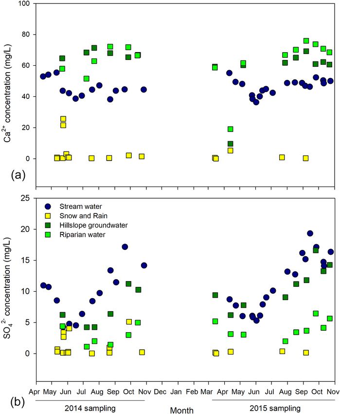
S. A. Spencer et al.: Hillslope and groundwater contributions to streamflow in a Rocky Mountain watershed                    241

stream water samples to support application of end-member        tion to collect the unsaturated soil water above the saturated
mixing analysis. Source water collection and sampling meth-      zone in the hillslope, which was sampled separately.
ods are detailed below.
                                                                 3.2.3   Hillslope groundwater
3.2.1   Rainfall and snowmelt
                                                                 Hillslope wells were installed with a shovel or hand auger
                                                                 to depth of refusal or maximum auger depth (1.5 m) near the
Rain samples were collected in clean buckets rinsed with
                                                                 hydrometric gauging stations at SEL, SEU, SWL, and SWU
deionized water. Buckets were placed in open areas through-
                                                                 (Fig. 1). A site was added at SEU at the end of the sum-
out the watershed or in the nearby townsite (Coleman, AB;
                                                                 mer in 2014, whereas the other sites were established during
within approximately 8 km of the Star Creek watershed) after
                                                                 summer 2013. Wells were installed in three locations at each
a rainstorm began. Locations were chosen opportunistically,
                                                                 site, namely riparian, toe slope, and hillslope positions, to de-
depending on storm timing and site access. Samples were
                                                                 termine the full range in hillslope groundwater. Well depths
collected at the end of the day or once there was enough wa-
                                                                 ranged between 0.5 m (riparian wells) and 1.6 m. Wells were
ter in the bucket to sample to prevent changes in chemical
                                                                 purged, using a hand pump, prior to sampling. Samples were
composition due to dry deposition of dust or evaporation. A
                                                                 collected approximately every 2 weeks, as available, between
total of five, four, and three samples were collected through-
                                                                 April and October in 2014 and 2015. Samples from the up-
out the summers of 2013, 2014, and 2015, respectively. The
                                                                 per hillslope wells were generally only obtained during the
difficulty in capturing large convective storms and the large
                                                                 snowmelt or high flow period; these wells were often dry
frequency of storms of less than 5 mm (Williams et al., 2019)
                                                                 during late summer. Riparian and toe slope wells contained
prevented the collection of more rainfall samples.
                                                                 water for all or most of the year, respectively. Water table
   A total of nine snowmelt samples were collected from the
                                                                 depths were monitored with capacitance loggers (Odyssey,
sub-alpine regions of Star Creek and two from North York
                                                                 Dataflow Systems Ltd., New Zealand) at 10 min intervals to
Creek (an adjacent watershed; Fig. 1) throughout spring and
                                                                 identify the timing of shallow groundwater table responses
early summer in 2014. Three additional samples were col-
                                                                 to infer potential periods when hillslope–stream connectivity
lected in spring 2015, but mid-winter melt of snowpacks
                                                                 occurred.
hindered the collection of more snowmelt samples. Eave-
stroughs, 3 m in length, were installed perpendicular to the
                                                                 3.2.4   Groundwater seeps
stream, with a small overhang off the edge of the hillslope
in Star Creek and North York Creek watersheds in the fall
                                                                 At the onset of this research, a lack of access to backcoun-
prior to snow accumulation. Samples were collected directly
                                                                 try sites restricted the installation of deep bedrock or till
from snowmelt troughs and snow bridges with clearly visi-
                                                                 groundwater wells in upper sub-watersheds. Rather, ground-
ble melt. Snowmelt was sampled, instead of the snowpack,
                                                                 water seeps were used to characterize the possible range in
to better reflect the meltwater signature during the snowmelt
                                                                 groundwater signatures (both bedrock and till groundwater)
period (Johannessen and Henriksen, 1978; Williams et al.,
                                                                 within Star Creek. Seeps are defined here as areas of visi-
2009). The timing of sample collection was based on access
                                                                 ble water seeping from hillslopes proximal to the stream or
to backcountry sites, and samples were taken opportunisti-
                                                                 from small wetland areas further from the stream that form
cally when crews were in the area and were able to observe
                                                                 small tributaries or rivulets that flow into the stream. The
active snowmelt.
                                                                 east and west forks were initially surveyed from the conflu-
                                                                 ence with the main stem to the stream origins in the alpine
3.2.2   Soil water                                               area in July 2013. A total of 25 visible seeps were identi-
                                                                 fied, which ranged in duration and magnitude of their con-
Suction lysimeters were installed between 30–60 cm depth         tributions to streamflow. Some seeps were only active during
using a hand auger in two locations near the toe of the hill-    the snowmelt season and recession period, reflecting stream-
slope in each sub-watershed in early spring 2014 (2015 for       flow dynamics. Other seeps were relatively stable throughout
SEU; Fig. 1). Suction lysimeters consisted of a 0.5 Bar ce-      the entire snow-free period or throughout the winter base-
ramic cup and 38.1 mm PVC pipe to ensure that ample water        flow period. Samples were collected during the following
was collected for chemical analyses. Water from the suction      three flow conditions: high flow (May/June), recession flow
lysimeter was sampled using a hand pump every 2 weeks be-        (mid-July), and baseflow (early September prior to fall rains),
tween April and October in 2014 and 2015. Suction lysime-        in both 2014 and 2015. This sampling campaign required
ters were pumped dry following sampling, and pressure was        more resources than for other sources; as a result, sampling
applied. Thus, soil water was composed of water that was         was completed only three times a year during the hydrolog-
able to pass through the ceramic cup over the 2-week period      ically important extreme flow conditions rather than every
until the lysimeter was at equilibrium pressure with the sur-    two weeks from April to October as for other sources. Wa-
rounding soil. Shallow depths were targeted with the inten-      ter temperature and electrical conductivity were measured

https://doi.org/10.5194/hess-25-237-2021                                         Hydrol. Earth Syst. Sci., 25, 237–255, 2021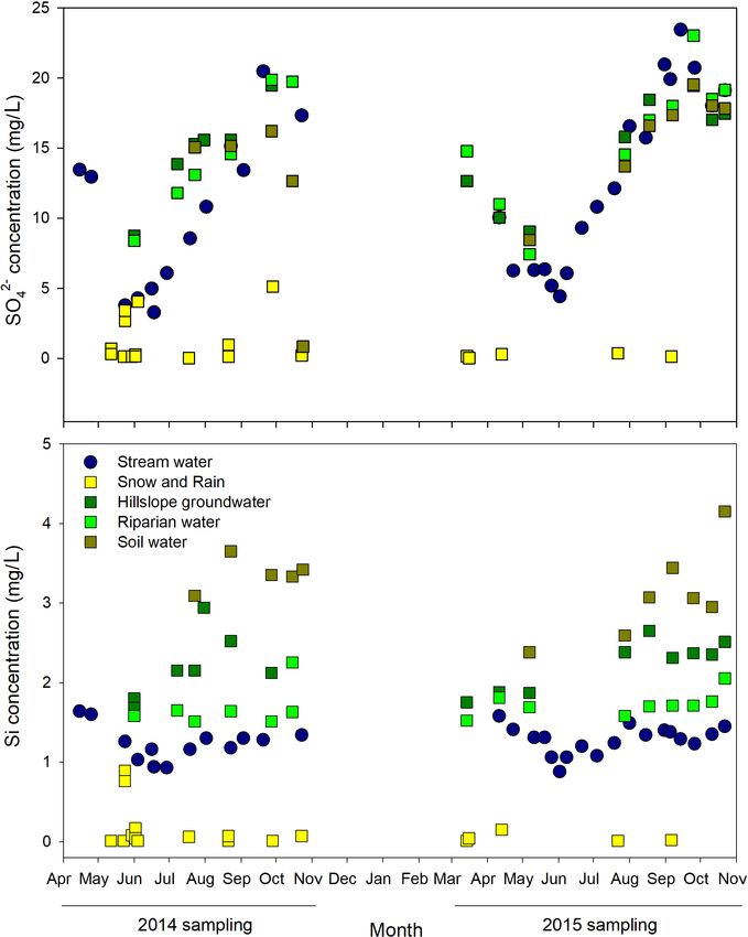
242        S. A. Spencer et al.: Hillslope and groundwater contributions to streamflow in a Rocky Mountain watershed

with a handheld multimeter (YSI85; YSI Inc. and Xylem             4   Data processing
Inc.; Yellow Spring, OH, USA) during sample collection to
aid in differentiating between deep bedrock groundwater, till     End-member mixing analysis (EMMA) was used to visualize
groundwater, and hillslope groundwater.                           multivariate source water and stream chemistry by reducing
                                                                  the dimensionality of the data with principal component anal-
3.2.5   Bedrock and till groundwater                              ysis (PCA; Christophersen and Hooper, 1992). In addition,
                                                                  there were multiple subjective decisions required prior to
Preliminary end-member mixing analysis showed that a wa-          EMMA, such as choosing tracers/ions and defining sources.
ter source was missing from those initially collected (above),    Bivariate plots and tracer variability ratio (TVR) were used
highlighting the need to characterize deeper groundwater.         to determine if tracers were appropriate to use in the analy-
Due to monetary and access limitations, a single borehole         sis. First, a matrix of bivariate plots of stream chemistry data
was drilled to 12 m depth (15.2 cm in diameter) in the to-        (ion concentrations), used most commonly in geographical
pographic ridge between SEL and SWL (approx. 500 m up-            hydrograph separations, was used to determine if ions were
stream from gauging sites) in October 2015 (Fig. 1). Two          conservative in nature (Hooper, 2003). A linear relationship
wells were installed in the borehole, one well in a water-        between tracers can be interpreted as a sign of conservative
baring formation in the bedrock at 11 m depth and a second        relationships. Second, TVR, used most commonly in sedi-
well in the glacial till deposits at 4.5 m depth, to character-   ment source apportionment studies, was used to determine
ize the differences in bedrock and till groundwater chem-         if the difference in ion concentrations between groups was
istry. Both wells had screens that were 1.5 m in length. Sand     larger than the variation within a source group (Pulley et al.,
was used to backfill the borehole around the screened sec-        2015). TVR was calculated using the following equation for
tion of the bedrock groundwater well and was capped with          each tracer and compared between each source group pair:
bentonite clay. Local material removed during drilling was
used to backfill the borehole up to the till layer. The same              x̃max −x̃min
                                                                              x̃min      × 100
method of back filling (sand, bentonite clay, and local mate-                                                                 (1)
                                                                  mean (CVsource 1 , CVsource 2 ) ,
rial) was used for the till groundwater well. Bedrock and till
wells were sampled every 2 to 4 weeks from April to Octo-         where x̃max is the maximum median tracer concentration of
ber in 2016 and 2017. Water in the till well was purged until     either source group, x̃min is the minimum median tracer con-
dry prior to sampling. Water in the bedrock well was purged       centration of either source group, and CV is the coefficient
for 2–5 min prior to sampling because the recharge rate was       of variation (Pulley et al., 2015; Pulley and Collins, 2018).
faster than the pump rate. Water table depth and tempera-         TVR should be greater than two to be considered appropri-
ture were measured continuously with pressure transducers         ate for use in mixing calculations (Pulley and Collins, 2018),
(HOBO U20; Onset Computer Corp., Bourne, MA, USA) at              although, depending on the data set in question, a greater
10 min intervals.                                                 threshold may be adopted to make the tracer selection more
   High concentrations of Na+ , Cl− , and SO2−
                                             4 in till ground-    stringent and to help reduce the numbers of tracers included
water (Fig. 3) and large variability between years suggested      in further data processing.
that the till groundwater well was likely contaminated by            Box and whisker plots and linear discriminant analy-
the bentonite clay used to backfill and seal between layers       sis (LDA) were used to remove the subjectivity of the defin-
(Remenda and van der Kamp, 1997). Slow recharge rates             ing sources (Ali et al., 2010; Pulley and Collins, 2018). Box
(and, therefore, low hydraulic conductivity) of glacial till      and whisker plots were used as a visual means of discrimi-
prevented the removal of three pipe volumes when sam-             nating between sources. LDA was then used to determine if
pling, and the corresponding low hydraulic conductivity re-       the combined sources exhibited sufficiently robust statistical
sulted in little flushing of bentonite contaminants. Faster       separation (Pulley and Collins, 2018). LDA optimizes sepa-
recharge rates (and, therefore, higher hydraulic conductiv-       ration between the centroid of group clusters by partitioning
ity) of the bedrock groundwater would aid in better flushing      the variation across each tracer and weighing that variation
of bentonite contaminants, which would reduce the effects         into two axes (reducing the dimensionality). Other statisti-
on bedrock groundwater chemistry (Remenda and van der             cal classification methods, such as hierarchical clustering or
Kamp, 1997). As a result, the till groundwater samples were       k-means clustering, were not appropriate because source cat-
not included in the analyses herein; however, water table         egories were known a priori. The data were processed in R
depths and water temperature dynamics could still be used to      (R Core Team, 2014), using the lda function in the MASS
understand the differences between till and bedrock ground-       package (Venables and Ripley, 2002) to reduce dimension-
water responses and their roles in runoff generation.             ality and assess the separation visually and the klaR (step-
                                                                  wise function; Weihs et al., 2005) package to model the data
                                                                  and determine the ability to separate groups statistically. The
                                                                  stepwise function models the data while removing individual
                                                                  tracers iteratively. The backwards direction was used in an

Hydrol. Earth Syst. Sci., 25, 237–255, 2021                                              https://doi.org/10.5194/hess-25-237-2021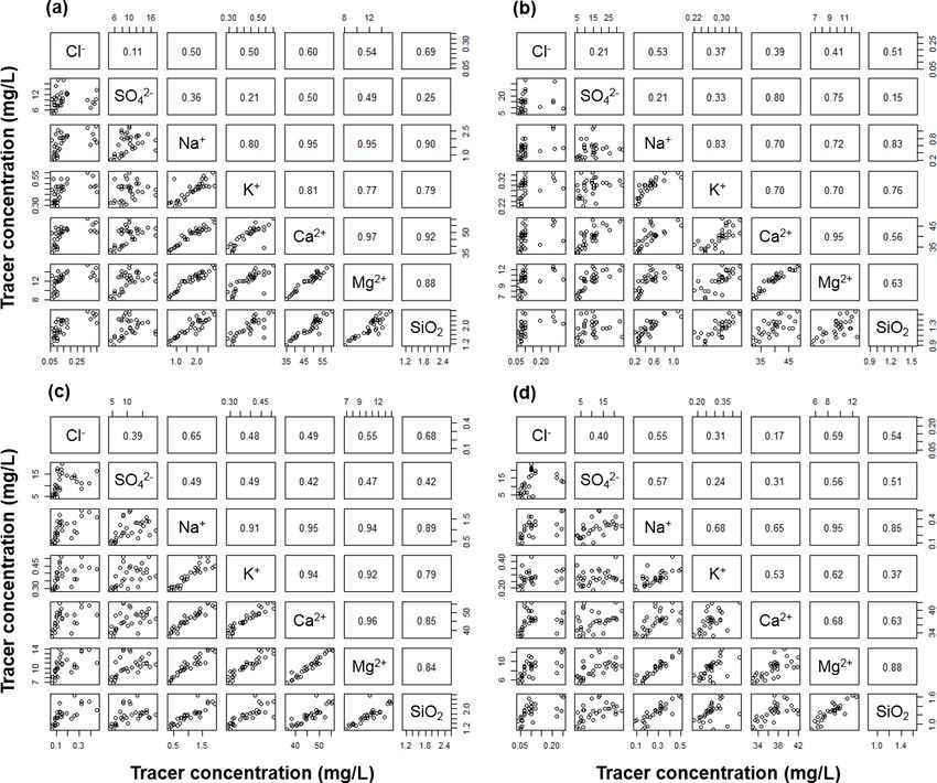
S. A. Spencer et al.: Hillslope and groundwater contributions to streamflow in a Rocky Mountain watershed                      243

Figure 3. Box plots for Star West Upper (SWU), Star East Upper (SEU), Star West Lower (SWL), and Star East Lower (SEL) showing the
ranges in chemistry for potential sources.

attempt to maintain the most tracers with the lda method and       tions. Source water was then standardized, using stream wa-
ability to separate criterion.                                     ter means and standard deviations for each ion, and projected
   After the sources were characterized, the stream water was      into the 2D mixing space as defined by the stream water
processed using principal component analysis (PCA; prcomp          (Christophersen and Hooper, 1992; Hooper, 2003). Stream
function in R; R Core Team, 2014) as a method of dimen-            water sources should create an outer boundary or polygon
sionality reduction to create a two-dimensional (2D) mix-          around all stream water samples if all sources were correctly
ing space (Christophersen and Hooper, 1992). Stream water          identified and adequately sampled.
was standardized (subtracting the mean and dividing by the
standard deviation for each sampling point) for each tracer,
to create equal variance between chemical components, and          5     Results
used to create a correlation matrix. PCA was conducted on
the correlation matrix to calculate eigenvectors and eigenval-     5.1    Tracer and source water group selection
ues. Standardized stream water was then projected into the
end member mixing space by multiplying by eigenvectors.            Bivariate plots were created, and TVR was calculated to de-
Ideally, two principal components (PCs) explained most of          termine which tracers were appropriate for use in EMMA.
the variation in the data and were used to generate a 2D mix-      Pearson correlation coefficients were calculated between all
ing space, which corresponds to three sources in EMMA              stream bivariate plots for stream water at each sub-watershed
(Hooper, 2003). Other studies have used the rule of one            (Fig. 4). These showed that all tracers exhibited acceptable
to determine how many dimensions, and therefore sources,           linear trends with at least one other tracer (Pearson’s r > 0.5;
should be used to create the mixing space (Ali et al., 2010;       p < 0.05) and were thereby likely conservative in nature.
Barthold et al., 2011). For this study, the mixing space was       TVR for almost all tracers at all sites were below two, with
set to two dimensions for ease of visualization but used all       the exception of precipitation group comparisons, which sug-
appropriate sources, as presented by Inamdar et al. (2013),        gested that the within-group variation exceeded the between-
to provide a full description of potential source contribu-        group variation for all subsurface sources. Greater variation
                                                                   within source groups compared to between source groups

https://doi.org/10.5194/hess-25-237-2021                                           Hydrol. Earth Syst. Sci., 25, 237–255, 2021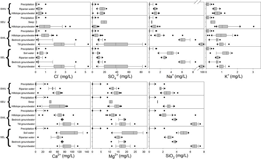
244        S. A. Spencer et al.: Hillslope and groundwater contributions to streamflow in a Rocky Mountain watershed

violates assumption 3 for EMMA (source water does not            The groundwater seeps mentioned above had low variabil-
change) and was considered unacceptable. As a result, rather     ity, like bedrock groundwater, but were cooler, suggesting
than calculating the mixing ratios or percent contribution of    potentially deeper bedrock groundwater sources than in the
sources to stream water on the basis of an unmixing routine      well. Temperatures of some other groundwater seeps were
in EMMA, trends in stream water distribution were described      more similar to bedrock groundwater although more vari-
in relation to source water dynamics and runoff processes.       able, ranging from 3.6 to 5.4 ◦ C (data not shown), while
   The a priori classification of water sources was rain,        others were more similar to till groundwater, ranging from
snowmelt, soil water, hillslope groundwater, till groundwater,   4.8 to 7.1 ◦ C (Fig. 5). The corresponding specific conductiv-
and bedrock groundwater; however, not all sites conformed        ity measurements add further complexity to these patterns.
to these categories. Box and whisker plots showed that the       The cool, temporally more stable seeps had low conductiv-
distribution of rain and snowmelt was too similar for them       ity from April to September, which was not reflective of
to be considered as separate groups. Although riparian wa-       the specific conductivity in the bedrock groundwater well.
ter mixes with stream water and should be chemically dif-        Rather, the other seeps with greater variability in tempera-
ferent from hillslope water as a source, soil water, toe slope   tures had high specific conductivity, which is more consistent
water, and upper hillslope water were grouped with riparian      with the bedrock groundwater wells (Fig. 5). Unfortunately,
water for most sites because the distribution of these sam-      the till-well-specific conductivity could not be used due to
ples were too similar to be considered separate sources. The     the contamination mentioned above, so it was unclear if the
exception was SEL and SWU, in which riparian water was           till groundwater had similar specific conductivity.
considered as a separate source. Final source water groups
are described below for each sub-watershed. LDA plots in-        5.2     Source water characterization
dicated that LD1 and LD2 explained 88.5 % and 11.5 %,
95.3 % and 4.7 %, 81.1 % and 15.5 %, and 77.6 % and 22.4 %       5.2.1    Star West source water
of the variance of the centroids for SWL, SWU, SEL, and
SEU sites, respectively. Stepwise analyses were also used in     Water sources for the SWL sub-watershed were grouped as
attempt to reduce the redundancy of the tracers and to ensure    precipitation (rain and snow), hillslope groundwater (soil wa-
that samples were well separated; on this basis, 99.7 %, 91 %,   ter, riparian water, and toe slope water), and bedrock ground-
98.6 %, and 99.9 % of samples were well separated in SWL,        water and plotted in PCA mixing space (Fig. 6). PC1 was
SWU, SEL, and SEU, respectively. In all sites, all tracers       mainly driven by cations, and PC2 was driven by anions (Ta-
were retained to maximize the ability to distinguish between     ble 1). Minimal variation in chemistry across all precipita-
the source groups. Overall, these results support the conclu-    tion samples (standard deviation (SD) of 2.4 and 1.1 for PC1
sion that there was good separation between the source water     and PC2, respectively) and overlap of snow and rain sam-
groups as they were recategorized for the individual sites.      ples in the mixing space confirmed that it was appropriate to
   At the outset of this research, groundwater seeps were        aggregate all samples (snow and rain) taken across all sites
sampled in lieu of bedrock and till groundwater wells to char-   (Star Creek, York Creek, and Coleman). Hillslope ground-
acterize the variability in the chemical signature of ground-    water exhibited greater chemical variation across samples
water throughout Star Creek. Most ion concentrations of the      (SD of 3.8 and 2.0 for PC1 and PC2, respectively) com-
groundwater seeps were not chemically distinct because they      pared to bedrock groundwater (SD of 2.9 and 4.8 for PC1
were generally similar to stream water or hillslope ground-      and PC2, respectively), but no clear temporal pattern was ob-
water in the PCA analyses (data not shown). However, the         served. Bedrock groundwater chemistry showed slight tem-
water temperature of groundwater seeps from spring to fall       poral variation, with more positive values in PC2 in the
revealed that some seeps were consistently cool while oth-       spring than in the fall.
ers had larger fluctuations in temperature. This suggests that      Water sources for the SWU sub-watershed were simi-
some seeps were potentially groundwater fed and others were      larly grouped as precipitation (rain and snow) and hillslope
fed by shallow subsurface water, respectively. For exam-         groundwater (soil water, toe slope water, and upper hillslope
ple, in SEL, the temperature of a groundwater seep ranged        water), but here riparian water displayed a greater difference
between 2.2 and 3.7 ◦ C throughout the summer (Fig. 5),          from hillslope groundwater and was considered as a sepa-
which is indicative of a bedrock groundwater source be-          rate source (Fig. 6). Bedrock groundwater samples were col-
cause the temperature range was muted and was largely            lected from a lower elevation in the watershed and may not
not influenced by radiative warming (Taniguchi, 1993). In        be representative of higher-elevation groundwater chemical
SEU, the temperature of a groundwater seep ranged from           composition; therefore, they were excluded from the anal-
2.5 to 3.5 ◦ C (Fig. 5), also indicating a bedrock groundwater   ysis for the upper sites. Furthermore, there were only two
source. Temperatures in the till groundwater well ranged be-     seeps identified in the upper watershed, but the temperature
tween 2.7 and 9.7 ◦ C, displaying some radiative heating and     and chemical composition of these seeps were not reflective
cooling, whereas the bedrock groundwater ranged between          of bedrock groundwater. While this did not exclude bedrock
5.1 and 5.8 ◦ C, displaying little radiative effects (Fig. 5).   groundwater contributions to streamflow in the upper regions

Hydrol. Earth Syst. Sci., 25, 237–255, 2021                                        https://doi.org/10.5194/hess-25-237-2021

S. A. Spencer et al.: Hillslope and groundwater contributions to streamflow in a Rocky Mountain watershed                                245

Figure 4. Bivariate plots of stream water chemistry at (a) Star East Lower, (b) Star East Upper, (c) Star West Lower, and (d) Star West Upper.
Top half of plots represents the Pearson’s correlation coefficient (r) for the linear relationship between each solute.

Table 1. Ions that explained the most variation in PC1 and PC2 for       of the watershed, it showed the chemical composition of the
each sub-watershed in Star Creek.                                        bedrock well, and the two seeps may not have been represen-
                                                                         tative of the bedrock groundwater chemistry in the Star West
            PC1        PC2                  PC1        PC2               Upper sub-watershed. Precipitation clustered tightly in one
   SEL      Mg (−)     SO4 (−)     SWL      Na (−)     K (−)             location, except for four snow samples and one rain sample,
            Si (−)     Cl (+)               Mg (−)     SO4 (+)           which increased the SD for precipitation (SD of 2.7 and 2.3
            Ca (−)                          Ca (−)     Cl (+)            for PC1 and PC2, respectively). All sources showed sim-
            Na (−)                          Si (−)                       ilar variation in precipitation; hillslope groundwater had a
            K (−)                                                        SD of 4.3 and 2.7 for PC1 and PC2, respectively, and ripar-
   SEU      Mg (−)     SO4 (−)     SWU      Mg (−)     Cl (+)            ian water had a SD of 3.0 and 2.0 for PC1 and PC2, respec-
            Ca (−)     Si (+)               Na (−)     Ca (−)            tively. A temporal pattern was observed for hillslope water
            Na (−)                          Si (−)     K (−)             in which hillslope water became less like precipitation from
            K (−)                                      SO4 (+)           spring to fall (Fig. 7). Temporal variation was also observed
                                                                         across months for riparian water and in which SO2− 4 concen-
                                                                         trations increased from spring to fall (Fig. 7).

https://doi.org/10.5194/hess-25-237-2021                                                  Hydrol. Earth Syst. Sci., 25, 237–255, 2021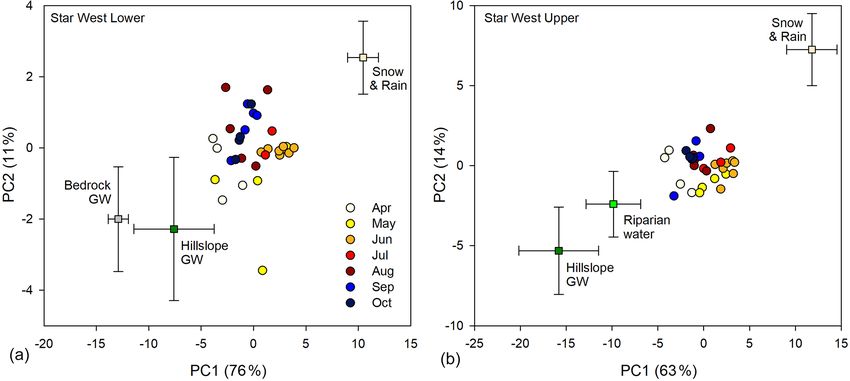
246 S. A. Spencer et al.: Hillslope and groundwater contributions to streamflow in a Rocky Mountain watershed
Figure 5. Box and whisker plot of groundwater, seep, and stream water temperature (a) and specific conductivity (b). Solid line indicates the
median, and the dashed line indicates the mean. The box indicates the 25th and 75th percentiles, the whiskers indicate the 90th percentiles,
and the circles indicate points within the 5th and 95th percentiles. Other seeps are shown here as an example of the temperature and specific
conductivity in many of the other seeps that were identified in the watershed but not used in the PCA biplots.
Figure 6. The first two principal components (PCs) of variation in stream water chemistry in Star West Lower (a) and Star West Upper (b)
from April to October (values in parentheses indicate the percent of variation explained by each PC). Square symbols indicate the mean
chemical composition (±1 SD – standard deviation) of stream water sources for each sub-watershed.
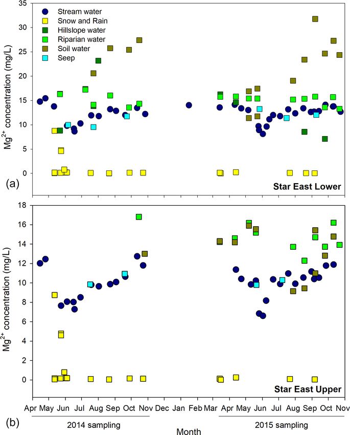
5.2.2 Star East source water water and varied from spring to fall (increased Ca2+ and
Mg2+ concentrations; Fig. 9). Riparian water was most simi-
Water sources for the SEL sub-watershed were grouped lar to stream water and did not vary over the season. A single
as precipitation (snow and rain), soil water, riparian water, groundwater seep that was chemically similar to stream wa-
groundwater seep, and bedrock groundwater (Fig. 8). Pre- ter, but for which temperatures were consistently cool, was
cipitation (SD of 1.4 and 1.1 for PC1 and PC2, respectively) retained to aid in the explanation of stream water dynamics
and bedrock sources (SD of 1.0 and 0.9 for PC1 and PC2, (Fig. 8).
respectively) were the same as those used in SWL. Hills- Water sources for the SEU sub-watershed were grouped
lope groundwater samples were initially grouped together as as precipitation (rain and snow), hillslope groundwater (soil
a single source, but high standard deviations and clustering water, riparian water, and toe slope water), and ground-
within the group suggested the separation of riparian water water seep (Fig. 8). Precipitation displayed little variation
(SD of 1.0 and 1.5 for PC1 and PC2, respectively) and soil (SD of 2.4 and 1.1 for PC1 and PC2, respectively). Large
water (SD of 4.3 and 1.5 for PC1 and PC2, respectively) into variation was observed for hillslope groundwater (SD of 9.3
individual sources. Soil water was most different from stream and 7.3 for PC1 and PC2, respectively). Toe slope water and
Hydrol. Earth Syst. Sci., 25, 237–255, 2021 https://doi.org/10.5194/hess-25-237-2021S. A. Spencer et al.: Hillslope and groundwater contributions to streamflow in a Rocky Mountain watershed 247
5.3.1 Star West stream water
The first two principal components (PCs) from the PCA anal-
ysis explained 87 % and 77 % of the variation in stream water
chemistry in SWL and SWU streams, respectively. Temporal
variation in stream water chemistry was constrained within
the broader multivariate mixing space created by the varia-
tion in source water chemistry but not within the more con-
strained mixing space of the mean composition (±1 SD) of
these sources (Fig. 6). In April, stream water was most simi-
lar to the hillslope groundwater (and riparian water in SWU).
Stream water transitioned through May to become the most
similar to precipitation source water in June (and July in
SWU). In SWL, stream water was slightly more similar to
hillslope groundwater and bedrock groundwater in July. In
August–October, stream water chemistry was more variable
and was similar to precipitation and hillslope and bedrock
groundwater. The temporal pattern associated with variation
in stream water chemistry through the fall was perpendicular
to the direction of the bedrock temporal pattern, suggesting
that hillslope groundwater (soil water, toe slope water, and ri-
parian water), rather than bedrock groundwater, was driving
the variation in stream water chemistry in the fall in SWL.
Time series of Ca2+ and SO2− 4 show that hillslope ground-
water was most similar to stream water (Fig. 10). Stream wa-
ter in SWU was again more chemically similar to hillslope
Figure 7. Time series of Si and SO2−
4 concentration in Star West groundwater and riparian water through August–October, but
Upper stream and source water in 2014 and 2015.
stream water chemistry differed slightly from its chemical
composition in the early summer months. Riparian water
riparian water had some chemical dissimilarities but were not chemistry had a similar temporal shift from April to Octo-
different enough from each other, or soil water, to be consid- ber as stream water chemistry, whereas hillslope groundwa-
ered as different groups. Some temporal variability was ob- ter and soil water had greater temporal variation (Fig. 7). Fur-
served in riparian water compared to SEL; however, soil wa- thermore, water table depth in the hillslope well indicates that
ter had much larger temporal variability than riparian water the upper hillslope is largely disconnected from the stream in
(Fig. 9). A single groundwater seep was identified in SEU. the fall in both SWL and SWU (Fig. 11), so it is more likely
The seep was chemically similar to stream water but tem- that the riparian area is contributing flow to the stream in the
peratures were consistently cool and indicative of a deep fall.
groundwater source, so it was retained to aid in the expla-
nation of stream water dynamics (Figs. 8 and 9). 5.3.2 Star East stream water
5.3 Stream water characterization Temporal patterns of variation in stream water chemistry ob-
served for SEL and SEU were very consistent with each
Stream water chemistry for all four sites showed high tem- other, again with the exception of the bedrock groundwater
poral variation throughout the months of open-water flow well, which was only sampled at a lower elevation site and,
(April–October) but little variation between years. As a re- therefore, not included in the PCA analysis in SEU. How-
sult, the temporal pattern of stream water was character- ever, seeps that displayed temporal stability in water tem-
ized for each site, in general, for 2014 and 2015 combined. perature typically characteristic of deep groundwater (Fig. 5)
Furthermore, due to the lack of source water samples dur- were used in the analysis for both SEL and SEU. The first two
ing winter months, the temporal pattern of stream water PCs explained 86 % and 83 % of the variation in stream wa-
was characterized from April to October, which represents ter chemistry in SEL and SEU, respectively (Fig. 8). For both
the most dynamic hydrologic period from the beginning of sub-watersheds, temporal variation in stream water chem-
snowmelt through to the start of the next year’s snow accu- istry was mostly constrained within the mixing space pro-
mulation period. Hydrologic characteristics of the 2014 and duced by the variation in source water chemistry, except dur-
2015 water years are indicated in Table 2. ing September/October when stream water plotted outside
this boundary. In April, stream water was most similar to the
https://doi.org/10.5194/hess-25-237-2021 Hydrol. Earth Syst. Sci., 25, 237–255, 2021248 S. A. Spencer et al.: Hillslope and groundwater contributions to streamflow in a Rocky Mountain watershed
Figure 8. The first two principal components of variation in stream water chemistry in Star East Lower (a) and Star East Upper (b) from
April to October (values in parentheses indicate the percent variation explained by each PC). Square symbols indicate the mean chemical
composition (±1 SD – standard deviation) of stream water sources for each sub-watershed.
Table 2. Streamflow and precipitation metrics for 2014 and 2015 water years.
2014 2015
SW SE SW SE
Annual precipitation (mm) 1149 1089 1091 1090
Annual discharge (mm) 944 648 719 468
Proportion of discharge May–July 0.69 0.74 0.45 0.54
Peak discharge (m3 s−1 ) 1.20 0.75 1.14 0.72
Average daily discharge∗ (m3 s−1 ) 0.14 (±0.20) 0.08 (±0.12) 0.10 (±0.10) 0.06 (±0.07)
∗ Standard deviation in parentheses.
riparian/hillslope water (or bedrock groundwater for SEL). 6 Discussion
The chemistry of stream water transitioned through May and
was most similar to precipitation in June. In July and Au- Twice monthly stream water and source water samples col-
gust, stream water became dissimilar from precipitation and lected in Star Creek, from April to October in 2014 and 2015,
was once again similar to riparian/hillslope water or bedrock have been used here to conceptualize runoff generation in
groundwater. In September and October, stream water was Alberta’s Rocky Mountains. Results from this study allow
less similar to riparian/hillslope water and plotted outside for a detailed examination of temporal patterns in source
the mixing space of the identified sources. Since stream wa- water chemistry and a qualitative description of source wa-
ter was not contained within the boundary created by the ter contributions to stream water. While our intention was a
source water, it is likely that an additional source was not quantitative estimate of source water contributions to stream-
captured by field sampling. However, the temporal variation flow using an unmixing routine, two of the key assumptions
in the chemistry of the groundwater seep followed the same for EMMA, the chemical composition of sources does not
pattern as the September/October stream water in both sub- change (1) over the timescale considered or (2) with space
watersheds, suggesting the same source water for the ground- (Hooper, 2003; Inamdar, 2011), were violated in this data
water seep and late fall baseflow (Fig. 8). Consistently cool set. Source water chemistry varied greatly across the water-
temperatures of the seep in SEL (2.2–3.7 ◦ C) and SEU (2.5– sheds. For example, when all hillslope samples from each
3.5 ◦ C) suggest a deeper groundwater source. sub-watershed were projected into the mixing space created
by stream water at the watershed outlet (SM), large vari-
ability was evident between sites (Fig. 12). While there was
some overlap between some sites (SWL and SEU), SWU
was clearly different than the other hillslope samples. As a
result, source water from within individual sub-watersheds
Hydrol. Earth Syst. Sci., 25, 237–255, 2021 https://doi.org/10.5194/hess-25-237-2021S. A. Spencer et al.: Hillslope and groundwater contributions to streamflow in a Rocky Mountain watershed 249
Figure 10. Time series of Ca2+ and SO2− 4 concentration in Star
Figure 9. Time series of Mg2+ concentration for Star East
West Lower stream and source water in 2014 and 2015.
Lower (a) and Star East Upper (b) stream and source water in 2014
and 2015.
of some tracer selection methods. Other studies have often
was used to reduce the uncertainty associated with large spa- used the selection criteria presented in Barthold et al. (2011),
tial variability in source water chemistry. However, the vari- but the unmixing routine is required for this method. Rather,
ability within sites was also quite large. The CV of source the TVR and LDA have been presented as effective param-
water tracer concentrations was often larger than the CV of eters to subjectively determine if tracers are included in the
the stream water tracer concentrations (there should be lit- analysis and if sources are well separated or grouped appro-
tle to no variation in source water over time; James and priately, respectively (Pulley et al., 2015, Pulley and Collins,
Roulet, 2006; Inamdar, 2011), particularly for K+ . The oc- 2018, and others – see the comprehensive review in Collins
casions where source water CV was smaller than stream wa- et al., 2017).
ter CV for most ions were for seeps in SEU and SEL, bedrock Despite the violation of assumptions, notable temporal
groundwater in SWL and SEL, and hillslope and riparian wa- trends in source water chemistry were observed in snowmelt,
ter in SWU. Chemical signatures of source water have been riparian water, hillslope and soil water, and bedrock ground-
shown to vary seasonally and annually (Rademacher et al., water and their contributions to stream water can be gener-
2005) and spatially across sub-watersheds in southern Que- alized for all sub-watersheds in Star Creek in a number of
bec, Canada (James and Roulet, 2006). As a result, James and ways. The water that was stored in the hillslope over win-
Roulet (2006) suggested that only source water from within ter (or reacted water) was likely the first to reach the stream
individual sub-watersheds of interest should be used in un- in the early spring prior to high flow as snowmelt started to
mixing calculations. Inamdar et al. (2013) further argued that saturate the landscape (Figs. 6 and 7). Temporal patterns in
mixing proportions should not be calculated because multi- stream water chemistry also showed a spike in concentra-
ple assumptions are often violated and can lead to significant tions of some ions (e.g., Ca2+ concentration in Fig. 11) in
errors in unmixing proportions. Rather, temporal and spatial the stream in the early spring, as this reacted water mobi-
variation in stream water and source water should be exam- lized prior to the onset of the snowmelt freshet. Although
ined and used to describe or to develop a physically based three snowmelt samples in 2014 showed similar ionic pulses
conceptualization of runoff mechanisms. early in the snowmelt season to those reported in the Col-
The inability to run the unmixing routine (stream water fell orado Rocky Mountains (Williams et al., 2009), the concen-
outside the bounds of the source water) also hindered the use trations were notably less than from all other sources and,
https://doi.org/10.5194/hess-25-237-2021 Hydrol. Earth Syst. Sci., 25, 237–255, 2021250 S. A. Spencer et al.: Hillslope and groundwater contributions to streamflow in a Rocky Mountain watershed
Figure 11. Observed inputs (snow depth and daily precipitation – estimated snow and rain proportions) and responses (stream discharge,
stream Ca2+ concentration, and shallow groundwater wells – hillslope and riparian) for Star Creek sub-watersheds in 2014 (left) and
2015 (right). Precipitation phase was separated into snow and rain after Kienzle (2008).
thus, not likely an important source of the observed early
season increase in stream water concentration of some ions.
Rather, the delivery of reacted water to the stream at the on-
set of snowmelt is likely similar to the flushing mechanism
observed in the Turkey Lakes watershed in central Ontario,
Canada (Creed and Band, 1998), where high nitrogen con-
centrations were observed prior to peak streamflow. McG-
lynn et al. (1999) observed the displacement of old water to
the stream at the onset of snowmelt in the Sleepers River re-
search watershed in Vermont, USA, and suggested this was
due to a small volume of snowmelt being added to a large
storage of water already in the subsurface.
This initial displacement of reacted water was followed by
a dilution effect, where large volumes of low-concentration
snowmelt mixed with soil water and contributed to stream-
flow. Snowmelt was the major event that produced a water
table response in all hillslope wells and connected the hill-
slopes to the stream (Fig. 11; Spencer et al., 2019). The initial
Figure 12. Hillslope groundwater from all sub-watershed sites in snowmelt period was also the only time that overland flow
2D mixing space, which was derived from a principal component was observed at the study site. Other studies have also re-
analysis of Star Main (Fig. 1) stream water. PC1 and PC2 represent
ported that snowmelt creates a dilution response in the stream
the first and second principal components.
(Rademacher et al., 2005; Cowie et al., 2017). Conversely,
the opposite has been observed whereby a previously dis-
connected source was connected to the stream and caused an
Hydrol. Earth Syst. Sci., 25, 237–255, 2021 https://doi.org/10.5194/hess-25-237-2021You can also read