The INSIEME seismic network: a research infrastructure for studying induced seismicity in the High Agri Valley (southern Italy) - Earth System ...
←
→
Page content transcription
If your browser does not render page correctly, please read the page content below
Earth Syst. Sci. Data, 12, 519–538, 2020
https://doi.org/10.5194/essd-12-519-2020
© Author(s) 2020. This work is distributed under
the Creative Commons Attribution 4.0 License.

        The INSIEME seismic network: a research infrastructure
                for studying induced seismicity in the
                    High Agri Valley (southern Italy)
        Tony Alfredo Stabile1 , Vincenzo Serlenga1 , Claudio Satriano2 , Marco Romanelli3 , Erwan Gueguen1 ,
              Maria Rosaria Gallipoli1 , Ermann Ripepi1 , Jean-Marie Saurel4 , Serena Panebianco1,5 ,
                                       Jessica Bellanova1 , and Enrico Priolo3
       1 Istitutodi Metodologie per l’Analisi Ambientale, Consiglio Nazionale delle Ricerche, Tito (PZ), 85050, Italy
             2 Université de Paris, Institut de physique du globe de Paris, CNRS, UMR 7154, 75238 Paris, France
              3 Centro di Ricerche Sismologiche, Istituto Nazionale di Oceanografia e di Geofisica Sperimentale,

                                                    Sgonico (TS), 34010, Italy
             4 Université de Paris, Institut de physique du globe de Paris, CNRS, UMS 3454, 75238 Paris, France
                 5 Università degli Studi della Basilicata, Dipartimento di Scienze, Potenza (PZ), 85100, Italy

                               Correspondence: Tony Alfredo Stabile (tony.stabile@imaa.cnr.it)

                                        Received: 28 June 2019 – Discussion started: 5 July 2019
                            Revised: 31 January 2020 – Accepted: 4 February 2020 – Published: 4 March 2020

      Abstract. The High Agri Valley is a tectonically active area in southern Italy characterized by high seismic
      hazard related to fault systems capable of generating up to M = 7 earthquakes (i.e. the 1857 Mw = 7 Basili-
      cata earthquake). In addition to the natural seismicity, two different clusters of induced microseismicity were
      recognized to be caused by industrial operations carried out in the area: (1) the water loading and unloading op-
      erations in the Pertusillo artificial reservoir and (2) the wastewater disposal at the Costa Molina 2 injection well.
      The twofold nature of the recorded seismicity in the High Agri Valley makes it an ideal study area to deepen
      the understanding of driving processes of both natural and anthropogenic earthquakes and to improve the current
      methodologies for the discrimination between natural and induced seismic events by collecting high-quality seis-
      mic data. Here we present the dataset gathered by the INSIEME seismic network that was installed in the High
      Agri Valley within the SIR-MIUR research project INSIEME (INduced Seismicity in Italy: Estimation, Moni-
      toring, and sEismic risk mitigation). The seismic network was planned with the aim to study the two induced
      seismicity clusters and to collect a full range of open-access data to be shared with the whole scientific commu-
      nity. The seismic network is composed of eight stations deployed in an area of 17 km × 11 km around the two
      clusters of induced microearthquakes, and it is equipped with triaxial weak-motion broadband sensors placed at
      different depths down to 50 m. It allows us to detect induced microearthquakes, local and regional earthquakes,
      and teleseismic events from continuous data streams transmitted in real time to the CNR-IMAA Data Centre. The
      network has been registered at the International Federation of Digital Seismograph Networks (FDSN) with code
      3F. Data collected until the end of the INSIEME project (23 March 2019) are already released with open-access
      policy through the FDSN web services and are available from IRIS DMC (https://doi.org/10.7914/SN/3F_2016;
      Stabile and INSIEME Team, 2016). Data collected after the project will be available with the permanent network
      code VD (https://doi.org/10.7914/SN/VD, CNR IMAA Consiglio Nazionale delle Ricerche, 2019) as part of the
      High Agri Valley geophysical Observatory (HAVO), a multi-parametric network managed by the CNR-IMAA
      research institute.

Published by Copernicus Publications.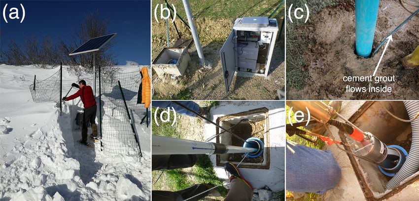
520                                                                          T. A. Stabile et al.: The INSIEME seismic network

1   Introduction                                                    ing the 1857 Mw = 7.0 Basilicata earthquake (Mallet, 1862;
                                                                    Burrato and Valensise, 2008), which was one of the most de-
Anthropogenic seismicity has been documented since the              structive historical earthquakes in Italy with 11 000 casualties
1920s when the subsidence due to the exploitation of the            and extensive damage throughout the Basilicata, Campania,
Goose Creek oil field (USA) was responsible for felt earth-         Apulia, and Calabria regions. It has also been estimated from
quakes (Pratt and Johnson, 1926). Today it is commonly              GPS velocity and strain rate field data (D’Agostino, 2014)
accepted that the term “induced seismicity” is synonymous           that the extensional opening in the axial part of the southern
with anthropogenic seismicity; therefore, in this paper the         Apennines is about 3 mm yr−1 .
two terms are considered interchangeable.                              The INSIEME seismic network was designed and devel-
   Considering the strong socioeconomic impact of induced           oped in the framework of the research project INSIEME (IN-
seismicity (for a complete review see National Research             duced Seismicity in Italy: Estimation, Monitoring, and sEis-
Council, 2013; Ellsworth, 2013; Grigoli et al., 2017; Foul-         mic risk mitigation), which was funded in 2015 by the SIR
ger et al., 2018; Keranen and Weingarten, 2018; Lee et al.,         (Scientific Independence of young Researchers) programme
2019), the current research in this field has twofold impor-        of the Italian Ministry of Education, Universities and Re-
tance: (a) from a social and economic point of view it is use-      search (MIUR) and ended on 23 March 2019. Two Italian
ful for addressing the range of issues related to the induced       test sites have been selected for the project’s research activ-
seismicity, including the development of specific “best prac-       ities: (a) the Collalto area in the municipality of Susegana
tice” protocols, monitoring strategies and traffic light sys-       (Veneto region, northeastern Italy), a site exploited by Edi-
tems, the correct definition of the associated hazard and risk,     son Stoccaggio S.p.A. for the storage of natural gas, and
and the discrimination between natural and induced seismic-         (b) the High Agri Valley (Basilicata Region, southern Italy)
ity; (b) from a purely scientific point of view the research is     hosting the biggest onshore oil field in western Europe, man-
fundamental for better understanding the processes involved         aged by Eni S.p.A., and the Pertusillo water reservoir. The
in earthquake generation; the interactions among rock, faults,      Collalto site has already been monitored since 2012 by a
and fluids as a complex system; and how perturbations of            dense network of 10 seismic stations and one permanent
the stress field, even of small size, may affect the stability of   GNSS geodetic station (https://doi.org/10.7914/SN/EV, Is-
faults over time. In order to achieve these two main goals, ad-     tituto Nazionale di Oceanografia e di Geofisica Sperimen-
equate monitoring networks should be deployed in the study          tale, 2012), which was the first Italian network providing data
area with the aim to obtain accurate earthquake locations and       with open-access policy (http://oasis.crs.inogs.it, last access:
to lower the completeness magnitude for generating huge mi-         January 2020; as reported in Priolo et al., 2015).
croseismic catalogues (Grigoli et al., 2017).                          In this paper, we present the INSIEME seismic net-
   On these grounds, in 2016 a dense seismic network                work and a detailed description of the acquired data which
(named INSIEME) was installed in the High Agri Valley               are released through open access. The broadband seis-
(hereinafter HAV), a NW–SE-trending intermontane basin              mic network has been registered at the International Fed-
formed during the Quaternary age along the axial zone of            eration of Digital Seismograph Networks (FDSN, http://
the southern Apennines thrust belt chain of Italy (Patacca          www.fdsn.org, last access: January 2020) with code 3F
and Scandone, 1989). Indeed, the area hosts energy tech-            (https://doi.org/10.7914/SN/3F_2016, Stabile and the IN-
nologies that cause two clusters of anthropogenic seismic-          SIEME Team, 2019). Section 2 details the seismic network
ity. More specifically, one of the two clusters (cluster A in       from its layout to the acquisition, transmission, and prelim-
Fig. 1) is continued-reservoir-induced seismicity (Ml ≤ 2.7)        inary processing of data. Section 3 is focussed on the de-
linked to the seasonal water level fluctuation of the artificial    scription of acquired seismic signals from the data quality of
Pertusillo Lake (Valoroso et al., 2009; Stabile et al., 2014a,      continuous data streams to the waveforms of recorded seis-
2015; Telesca et al., 2015; Vlĉek et al., 2018); the other clus-   mic events. Section 4 provides information on data availabil-
ter (cluster B in Fig. 1) is fluid-injection-induced seismicity     ity. Finally, our discussions and conclusions are reported in
(Ml ≤ 2) due to the disposal of the wastewater produced dur-        Sect. 5.
ing the exploitation of the biggest onshore oil and gas field in
western Europe at the Costa Molina 2 (CM2) injection well
(Stabile et al., 2014b; Improta et al., 2015, 2017; Wcisło et       2   The INSIEME seismic network
al., 2018). Furthermore, the HAV is one of the areas of Italy
with the highest seismic hazard with an expected maximum            The INSIEME seismic network has been designed to achieve
acceleration (referring to average hard ground conditions) for      two main purposes: (a) to study the seismic processes re-
an exceedance probability of 10 % in 50 years within 0.25           lated to the occurrence of events belonging to the two clusters
and 0.275 g according to the national reference seismic haz-        of anthropogenic seismicity and (b) to provide the scientific
ard model (Gruppo di Lavoro MPS, 2004). Indeed the Italian          community with new open-access high-quality seismic data
historical seismicity catalogue CPTI11 (Rovida et al., 2011)        for studying such phenomena and for developing method-
reports seven earthquakes with Mw ≥ 4.5 in the HAV, includ-         ologies useful to discriminate between natural and anthro-

Earth Syst. Sci. Data, 12, 519–538, 2020                                             www.earth-syst-sci-data.net/12/519/2020/
T. A. Stabile et al.: The INSIEME seismic network                                                                                       521

Figure 1. Layout of the INSIEME seismic network in the High Agri Valley. Cyan triangles represent the eight broadband seismic stations
of the network. Yellow and orange triangles represent stations belonging to private (i.e. the Eni Company) and public seismic monitoring
networks, respectively. The CM2 injection well is depicted with a black dot inside a grey circle. Natural and anthropogenic earthquakes are
represented with red circles (2002–2012 seismicity from Serlenga and Stabile, 2019). Anthropogenic seismicity is classified as seismicity
induced by continued reservoir (clusters A) and fluid injection (cluster B). The map was drawn using Matplotlib Python library (Hunter,
2007), which incorporates the ArcGIS REST Services freely available at http://server.arcgisonline.com/arcgis/rest/services (last access: Jan-
uary 2020).

pogenic events. The following points provide details of the                   the event depth (Havskov et al., 2012). These two condi-
network from its layout to the data acquisition and process-                  tions allow for a good control of event depth estimation.
ing.
                                                                            – High-quality sites, possibly on hard bedrock and there-
                                                                              fore without local ground effects, should be selected.
2.1   Seismic network layout

The INSIEME network is composed of eight stations cover-                    – Recommended station locations must be as far as pos-
ing an area of about 17 km × 11 km, organized in two groups                   sible from strong noise sources such as main roads,
of four stations around each of the two clusters of anthro-                   town centres, industrial, and quarry activities which are
pogenic events (red circles in Fig. 1). All the stations are                  largely diffused in the HAV.
equipped with broadband sensors installed in non-toxic PVC
(polyvinyl chloride) casings at different depths down to 50 m.              – Station sites must be accessible for drilling operations.
Network layout and design definition were driven by several
constraints, hereafter summarized.                                          – In areas belonging to the national park “Val d’Agri –
                                                                              Lagonegrese”, which covers large portions of the HAV
  – Seismic stations must be deployed around the two clus-                    territory (see file “INSIEME-network.kmz” provided in
    ters of induced events with as uniform as possible az-                    the Supplement), it is not possible to drill boreholes.
    imuthal distribution.
                                                                            – Station sites should be covered by the 3G mobile com-
  – Taking into account that the studied clusters are charac-                 munication link.
    terized by shallow events of about 4–5 km focal depth
    (Serlenga and Stabile, 2019), the epicentral distance of                – Seismic stations should guarantee continuous data ac-
    the closest station must be less than the focal depth of                  quisition in all weather conditions, even in the winter
    events belonging to such seismicity clusters, and the av-                 season when the snow coverage could reach up to 1.5–
    erage distance between stations should not exceed twice                   2.0 m thickness for a couple of weeks.

www.earth-syst-sci-data.net/12/519/2020/                                                    Earth Syst. Sci. Data, 12, 519–538, 2020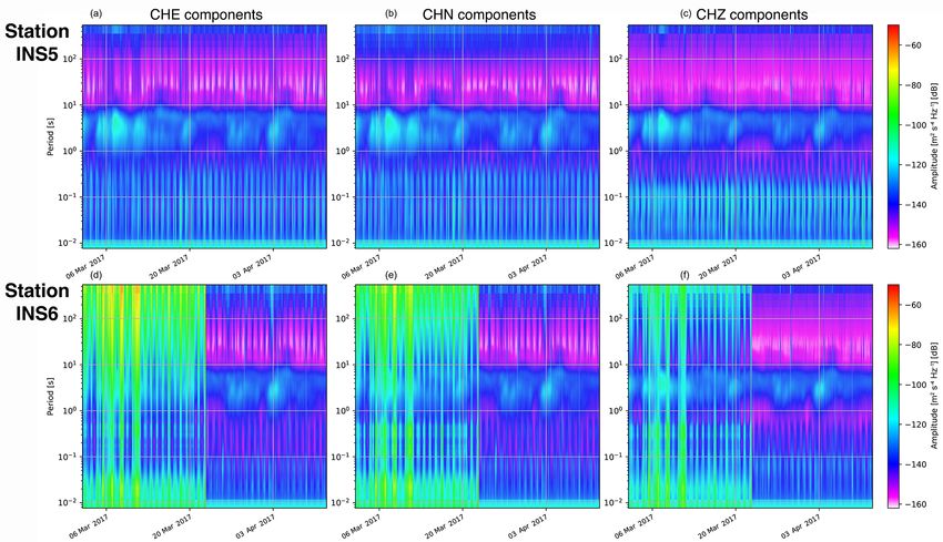
522                                                                         T. A. Stabile et al.: The INSIEME seismic network

  – With the aim to provide an effective added value to the
    seismic monitoring of the HAV, station locations should
    not overlap existing stations of operating public and pri-
    vate seismic networks.

We performed seismic ambient noise measurements and geo-
logical surveys in order to find the most suitable sites accord-
ing to these constraints, and we verified the access to the site
(also for drilling operations of the shallow boreholes), data
transmission conditions, and unexpected potential sources of
local noise. We evaluated the network performances follow-
ing the approach proposed by Stabile et al. (2013) by con-
sidering different configurations of the potential sites that
have met as many constraints as possible. The final net-
work configuration is reported in Fig. 1. It is worth noting
that the minimum distance between station (cyan triangles in
Fig. 1) ranges between 2.7 km (INS6 and INS7 stations) and
                                                                   Figure 2. Amplitude and phase response curves for the INS1 station
5.4 km (INS1 and INS4), the distance of the closest station to     (blue curves), equipped with a 0.0083–100 Hz TCPH seismometer,
each cluster is less than 4–5 km (the focal depth of induced       and for the INSX station (orange curves), equipped with a 0.05–
events), and the INSIEME stations do not overlap stations be-      100 Hz TCPH seismometer. The sensor sensitivity at 1 Hz is also
longing to other public (orange triangles in Fig. 1) and private   reported. The vertical dotted green line indicates the Nyquist fre-
(yellow triangles in Fig. 1) seismic networks. Only the INS8       quency of 125 Hz.
station falls in the national park Val d’Agri – Lagonegrese
area and, therefore, the sensor of this station was installed on
the surface.                                                       Cemetery, power supply for all stations is provided by solar
                                                                   panels and batteries. Each station is equipped with a 270 W
2.2   Seismic stations                                             solar panel and two 12 V, 100 Ah batteries connected in se-
                                                                   ries to output 24 V, which allow the instruments to work with
Considering that the main target of the INSIEME network is         less current. Solar panels are installed on 2 m high poles
to detect and locate the anthropogenic microseismicity in the      in order to prevent snow covering during the winter season
HAV (Ml ≤ 2.7), the seismic stations were equipped with tri-       (see Fig. 3a). The solar charge controller, the two batteries,
axial weak-motion broadband sensors: six 0.05–100 Hz and           the power supply circuit, the data logger, and the router are
two 0.0083–100 Hz Trillium Compact Posthole (TCPH) seis-           housed in a small cabin (Fig. 3b). Corrugated cables allow
mometers. The data loggers are Centaur digital recorders           the passage of sensor cables from the cabin to the borehole
with a dynamic range of 140 dB. All seismometers and data          (Fig. 3b). Each borehole is closed by a manhole (Fig. 3b) and
loggers are manufactured by Nanometrics Inc. (see Table 1).        the PVC casing is coupled to the soil by cement grout filling
Continuous acquisition of digital waveforms is provided by         the space between the hole and external surface of the PVC
the INSIEME network at a 250 Hz sampling rate. This choice         casing from the bottom to the surface (Fig. 3c). The PVC
allows data acquisition with a Nyquist frequency of 125 Hz         casing is not in the manhole in order to leave room for in-
(Fig. 2), which is greater than the upper frequency bound          stalling sensors on the surface (Fig. 3d). A 2 m high netting,
of the broadband sensors (100 Hz), thus avoiding the appli-        surrounding an area of about 2.5 m×2.5 m, protects each sta-
cation of temporal anti-aliasing filters to the acquired sig-      tion from wild or grazing animals.
nals and taking advantage of the high-frequency bound pro-            The broadband seismometers installed in boreholes are
vided by the sensors useful to capturing the full spectra          equipped with a coupling system (Fig. 3e), developed by the
content of small earthquakes. The amplitude and phase re-          National Institute of Oceanography and Experimental Geo-
sponses of the two versions of broadband sensors are shown         physics of Italy (OGS), which fastens the sensor to the bore-
in Fig. 2: blue curves refer to the INS1 station (equipped with    hole wall. The inclination of each borehole from the sur-
a 0.0083–100 Hz TCPH seismometer) and orange curves                face to the bottom has been measured with an in-place in-
refer to the INSX station (equipped with a 0.05–100 Hz             clinometer (Jewell Instruments, model 906 “Little Dipper”).
TCPH seismometer). The first installed station of the net-         We found that the five shallow boreholes of 6 m depth (sta-
work was INSX (in operation between 1 April 2016 and               tions INS2, INS3, INS4, INS5, and INS6) have inclination at
24 January 2017) whereas the other stations have been in-          the bottom of less than 1◦ and one of the two 50 m deep bore-
stalled since 23 September 2016 (see Table 2).                     holes deviates 1.6◦ at the bottom (station INS1). Concerning
   With exception of the INS1 station which was initially          the second 50 m deep borehole (station INS7), the inclina-
connected to the electric power grid of the Montemurro             tion of the borehole becomes greater than 2◦ at depths greater

Earth Syst. Sci. Data, 12, 519–538, 2020                                             www.earth-syst-sci-data.net/12/519/2020/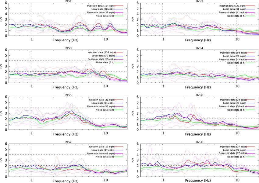
T. A. Stabile et al.: The INSIEME seismic network                                                                                     523

Table 1. Geographic coordinates and elevation of the INSIEME broadband seismic stations with indication of the sensor type installed at
each station (TCP: Trillium Compact Posthole).

                                  Station      Latitude     Longitude    Elevation     Sensor
                                  name              ◦N            ◦E      (m a.s.l.)   type
                                  INSX       40.305686      15.989105          806     20 s–100 Hz TCP
                                  INS1       40.305790      15.988603          802     120 s–100 Hz TCP
                                  INS2       40.342090      15.951559         1043     20 s–100 Hz TCP
                                  INS3       40.328033      16.034446          880     20 s–100 Hz TCP
                                  INS4       40.278168      16.040405          652     20 s–100 Hz TCP
                                  INS5       40.275704      15.906211          602     20 s–100 Hz TCP
                                  INS6       40.229581      15.887608          745     20 s–100 Hz TCP
                                  INS7       40.221487      15.917465          881     120 s–100 Hz TCP
                                  INS8       40.241083      15.972221          882     20 s–100 Hz TCP

Table 2. Position of the broadband sensors during time for each station with the indication of the sensor depth when it is installed in the
borehole.

                      Station name                Surface                         Borehole              Sensor depth
                                       Installation   Uninstallation    Installation   Uninstallation
                      INSX            2016-04-01          2017-01-24             –                 –              –
                      INS1                     –                   –    2016-10-12                 –           50 m
                      INS2            2016-09-23          2017-03-22    2017-03-22                 –            6m
                      INS3            2016-08-26          2017-03-22    2017-03-22                 –            6m
                      INS4            2016-08-26          2017-03-22    2017-03-22                 –            6m
                      INS5            2016-08-26          2016-10-13    2016-10-13                 –            6m
                      INS6            2016-08-26          2017-03-22    2017-03-22                 –            6m
                      INS7            2017-03-02          2017-03-23    2017-03-23                 –           14 m
                      INS8            2017-03-02                   –             –                 –              –

than 20 m. Indeed, at 14 m depth we measured an inclination             station by applying a methodology similar to that proposed
of 1.7◦ , increasing up to 2◦ between 16 and 20 m, and over             by Zheng and McMechan (2006), based on the maximization
6◦ beyond 24 m depth. Since the two deeper boreholes host               of the cross-correlation among the horizontal traces of adja-
the 0.0083–100 Hz TCPH seismometers which operate with                  cent sensor pairs. Of course, for each pair of adjacent sen-
a maximum tilt of 2◦ , we installed the seismometer of sta-             sors we assume the condition of plane wave approximation
tion INS1 at 50 m depth whereas the INS7 one was installed              which is satisfied if the distance d between sensors is much
at 14 m depth. Table 2 indicates the sensor depths of each              less than the dominant wavelength λ of the recorded signal
borehole station.                                                       (d  λ). Therefore, the signals recorded by the two sensors
   The seismometers at 6 m depth were installed by a mod-               must be filtered with a cut-off frequency fc  V d −1 , with V
ular non-rotating pipe system developed by OGS in or-                   the lowest seismic velocity of the medium.
der to control the orientation of the horizontal components                For each angle θ ranging from 0 to 360◦ with a step size of
(Fig. 3d). The non-rotating system consisted of a set of con-           0.5◦ , we computed the normalized cross-correlation between
nectable, light, and rigid pipes, 3 m long and 50 mm outside            the north component of the signal recorded by the reference
diameter, equipped with a mating joint at the velocimeter end           station (SrN ) and the first horizontal component of the signal
and a reference mark at the top, thus allowing us to push the           recorded by sensor with unknown orientation and rotated an-
sensor sled and, at the same time, set the correct azimuthal            ticlockwise by the angle θ (Suθ1 ). In addition, we computed
angle. After the installation was completed we released the             the normalized cross-correlation between the east component
joint by lifting and removing the tubes, and the sensor stands          of the signal recorded by the reference station (SrE ) and the
were undisturbed. For the two seismometers placed at 14 and             second horizontal component of the signal recorded by sen-
50 m depth, respectively, the orientation of their horizontal           sor with unknown orientation and rotated anticlockwise by
components was unknown because of the impossibility of                  the angle θ (Suθ2 ). For each angle θ , the maximum values of
using a longer non-rotating pipe system. In this case we esti-          the cross-correlation between SrN and Suθ1 (Aθ ) and between
mated their azimuthal orientation with respect to a reference           SrE and Suθ2 (B θ ) were retrieved. Then, the sensor orienta-

www.earth-syst-sci-data.net/12/519/2020/                                                     Earth Syst. Sci. Data, 12, 519–538, 2020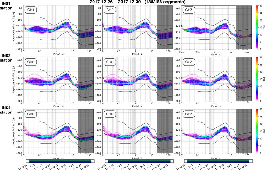
524 T. A. Stabile et al.: The INSIEME seismic network
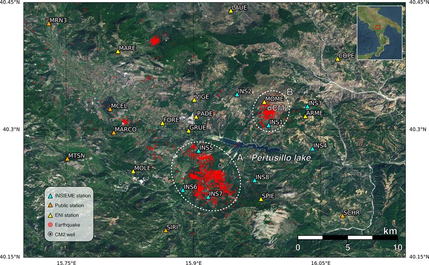
Figure 3. Details of a typical seismic station of the INSIEME network: (a) the solar panel is installed on a pole of 2 m height in order to
prevent it being covered by snow during the winter season; (b) all the instruments of a station are housed in a small cabin which is connected
to the borehole where the seismometer is installed inside a PVC casing; (c) the PVC casing is coupled to the soil using cement grout; (d) the
PVC casing is not centred in order to leave space for installing sensors on the surface, and seismometers placed at 6 m depth are installed by
using a non-rotating pipe system; (e) all the broadband seismometers installed in boreholes are equipped with a coupling system.
tion with respect to the reference sensor was given by the angle for the sensor of station INS1 is 307.8±0.4◦ anticlock-
following Eq. (1): wise to the north.
For station INS7 we used as reference the station INS1
θ BEST = θ : Aθ B θ , after its alignment to the north because the two stations are
max (1)
0◦ ≤θ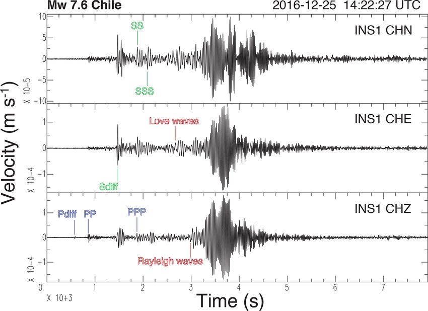
T. A. Stabile et al.: The INSIEME seismic network                                                                            525

tem) whose host name is linked up to the router’s dynamic IP          In the CNR-IMAA Data Centre there is a Linux server for
address. In this way the end user is able to directly reach each   data acquisition, storage, and processing. The server has been
seismic station, for both management and data acquisitions.        equipped with a hardware RAID controller (redundant array
   The use of the dynamic DNS system instead of a VPN              of independent discs), configured as a “RAID 1” disc mirror-
system such as OpenVPN was a technical choice because              ing, to protect the data in case of drive failure. Our configu-
the latter requires a dedicated server and configuration. The      ration features two 4 TB hard discs (i.e. 8 TB RAW space) in
dynamic DNS is also supported by other routers already in          RAID 1 mode, ensuring a N + 1 disc redundancy and a 4 TB
our warehouse (typically TP-LINK, which does not support           total storage capacity. This configuration is an optimal choice
VPN) which can temporally replace a Teltonika in case of           for applications requiring high availability. In the future, we
failure.                                                           will upgrade the system by means of network-attached stor-
   The Nanometrics Centaur digital recorder uses a data            age (NAS) in order to store data as well as to enhance the sys-
streaming protocol called SeedLink (https://ds.iris.edu/ds/        tem performance and availability. Furthermore, on this server
nodes/dmc/services/seedlink, last access: January 2020).           the TCP/IP-based SeedLink standard compliant SeisComP3
This is a transmission protocol system used to make the            (https://www.seiscomp3.org, last access: January 2020) soft-
data available on the Internet, based on the “Internet Pro-        ware runs for seismological data acquisition. It acquires
tocol suite TCP/IP” (Transmission Control Protocol/Internet        data in real time from the INSIEME stations and neigh-
Protocol) standard.                                                bour stations, stores them in a miniSEED file structure, and
   Since it is not uncommon for routers to encounter prob-         is able to make those data available through various stan-
lems causing the interruption of the internet connection, each     dard protocols: SeedLink for real-time flow, ArcLink (https:
station is equipped with two automatic reboot systems. The         //www.seiscomp3.org/doc/applications/arclink.html, last ac-
first one is integrated inside the router and based on a ping      cess: January 2020) and FDSN web services (https://www.
utility: if the system does not ping an external public IP for     fdsn.org/webservices, last access: January 2020) for archived
some time, the router is automatically rebooted. The sec-          data requests. This SeisComP3 software also holds the sta-
ond one is based on an external programmable time switch           tions’ metadata and an event database. A schematic view of
which periodically (in our case once a week) unplugs the           the data flow from the data logger to the data centre is dis-
power supply of the router for a few seconds, thus preventing      played in Fig. 5.
any software bug that could freeze the Teltonika. When the            A dedicated web-based system, WebObs (Beauducel et
router restarts, the Centaur data logger is able to send miss-     al., 2020), is used to plot a numerical strip chart (called
ing data to the CNR-IMAA (National Research Council of             “SefraN”) of a representative subset of the configured sta-
Italy, Institute of Methodologies for Environmental Analy-         tions in near real time. SefraN is used to manually iden-
ses) Data Centre. Despite these precautions, sometimes data        tify any event present in the data (Fig. 6, top panels). It is
gaps may occur due to prolonged temporary absence of the           associated with the Daybook, a database of all the events
3G signal or other minor transmission problems. For this rea-      that have been identified in the data, whether they can be
son, a 16 GB SD memory card is mounted on each Centaur             located or not, based on the availability of both P- and S-
which allows the local storage of about 6 months of data. Af-      wave pickings. Some regional and global events are prefilled
ter a check on data availability using the vertical component      with information gathered from INGV (http://terremoti.ingv.
data stream of each station for the entire period of opera-        it/webservices_and_software, last access: January 2020) and
tion of the INSIEME seismic network (Fig. 4), the available        USGS (https://earthquake.usgs.gov/fdsnws/event/1/, last ac-
data range between 93.8 % (INS6 station) and approximately         cess: January 2020) FDSN event web services. When a new
100 % (INS2, INS3, INS7, and INS8 stations). All the gaps          event is identified, the information is sent to the SeisComP3
due to transmission problems have been filled by using data        database (Fig. 6). The event is then manually picked and lo-
saved on each SD memory card. The unfilled gaps are re-            cated (Fig. 6, bottom panel) with SeisComP3 Origin Locator
lated to a programmed temporary shutdown of a station (e.g.        Viewer (scolv), using the 1-D velocity model from Improta
maintenance, firmware update) or to undesired problems oc-         et al. (2017). The WebObs Daybook displays the event infor-
curring at a specific station. As an example, the missing data     mation collected from the SeisComP3 FDSN web service.
of station INS6 of about 6.2 % (corresponding to a cumu-           A preliminary catalogue of HAV seismicity from Septem-
lative time of about 58 out of 940 d) are due to a miscon-         ber 2016 to March 2019 has been produced and is avail-
figuration of the solar charge controller on which the night       able at https://doi.org/10.5281/zenodo.3632419 (Stabile et
light function was erroneously activated (during sunshine the      al., 2020).
power was switched off). The problem was understood and
definitively solved on 24 January 2017 at 09:52 UTC. After
this configuration correction, the gaps at station INS6 have
become comparable to those observed at the other stations of
the INSIEME seismic network (Fig. 4).

www.earth-syst-sci-data.net/12/519/2020/                                             Earth Syst. Sci. Data, 12, 519–538, 2020
526                                                                               T. A. Stabile et al.: The INSIEME seismic network

Figure 4. Data availability (blue lines) for all stations for the entire period of operation of the INSIEME seismic network. The analysis has
been performed on the vertical component data stream of each station (CHZ channels). The percentage of data availability is reported below
each station name.

Figure 5. Schematic view of the data flow from the data logger of a remote station to the CNR-IMAA Data Centre.

3     Acquired seismic signals                                              It is well known that the background noise is due to sev-
                                                                         eral factors like temperature changes, weather conditions,
3.1    Data quality in terms of background noise level                   and anthropogenic noise. The first two factors generally pro-
                                                                         duce low-frequency noise (< 0.05 Hz) whereas the last usu-
One of the most important goals of a seismic network is to
                                                                         ally contains high frequencies (> 1 Hz). In addition there is
provide high-quality records of a seismic event from a num-
                                                                         also the microseismic noise in the range 4–8 s generated by
ber of stations as large as possible and with a good azimuthal
                                                                         the sea activity (Longuet-Higgins, 1950). Since most of the
coverage; therefore, if the seismic noise is high at different
                                                                         broadband sensors of the INSIEME seismic network have
sites, the benefits of modern equipment with a large dynamic
                                                                         a flat response in the range 0.05–100 Hz (see Table 1) and
range are compromised (Havskov et al., 2012).
                                                                         the seismic network is primarily designed to observe mi-
                                                                         croearthquakes, the main goal of our sensor installations is

Earth Syst. Sci. Data, 12, 519–538, 2020                                                   www.earth-syst-sci-data.net/12/519/2020/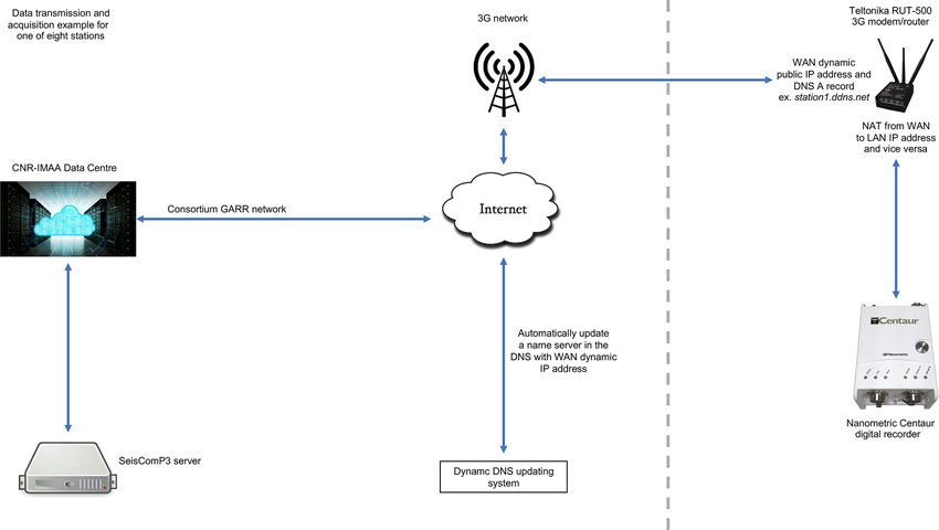
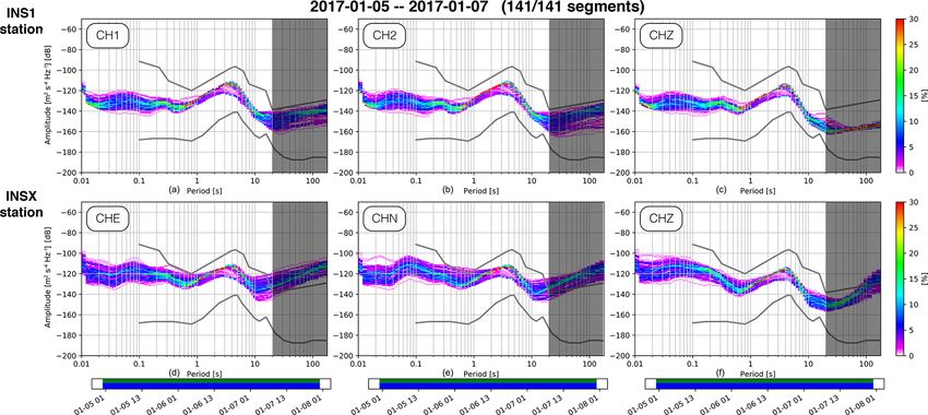
T. A. Stabile et al.: The INSIEME seismic network                                                                                 527

                                                                       5 to 7 January 2017, characterized by high natural and an-
                                                                       thropogenic noise level, we computed the probabilistic power
                                                                       spectral densities (McNamara and Buland, 2004). Figure 7
                                                                       shows the comparison of the probabilistic power spectral
                                                                       densities (hereinafter PPSDs) obtained for each component
                                                                       of INS1 and INSX stations in the period range 0.01–20 s (fre-
                                                                       quency range 0.05–100 Hz). The colour palette indicates the
                                                                       probability (in percentage) of having a certain noise level as a
                                                                       function of the period. The two grey lines in each panel indi-
                                                                       cate the new high- and low-noise models, obtained by Peter-
                                                                       son (1993), which are used as reference. The two horizontal
                                                                       components of INS1 station (CH1 and CH2, according to the
                                                                       SEED channel naming standard; https://ds.iris.edu/ds/nodes/
                                                                       dmc/data/formats/seed-channel-naming, last access: January
                                                                       2020) are compared with the two horizontal components of
                                                                       INSX station (CHE and CHN), and the vertical components
                                                                       (CHZ) of the two stations are compared to each other. It is
                                                                       possible to observe that the noise level is less widespread at
                                                                       50 m depth than at surface and that for periods below 1 s (fre-
                                                                       quencies above 1 Hz) we have a reduction of the noise level
                                                                       of about 10 dB on average and up to 20 dB. In Fig. 7, peri-
                                                                       ods above 20 s (frequencies below 0.05 Hz) are highlighted
                                                                       in grey because in such a period range it is not possible to
                                                                       compare the PPSDs of the two stations since only the sen-
Figure 6. Tools implemented for visualization and processing of
                                                                       sor of the INS1 station has a flat response up to 120 s (see
acquired seismic data. The WebObs system (top panels) is used to
plot a strip chart of recordings at configured stations in near real
                                                                       Table 1) and, therefore, only its PPSD is significant.
time for any event present in the data. When an event is identified,      We also computed the PPSD on continuous data streams
the information is sent to the SeisComP3 database for the manual       acquired by the INS1, INS2, and INS4 stations from 26 to
phase picking and event location (bottom panel) through the Origin     30 December 2017, a period again characterized by high nat-
Locator Viewer tool (scolv).                                           ural and anthropogenic noise levels. It is possible to note (Ta-
                                                                       ble 2) that the INS2 and INS4 stations are equipped with
                                                                       sensors installed at 6 m depth. Figure 8 shows the compar-
to attenuate the anthropogenic noise. Several studies have al-         ison among the PPSDs obtained for the horizontal and verti-
ready focused on the attenuation of such a specific kind of            cal components of each station in the period range 0.01–20 s
noise (Young et al., 1994; Withers et al., 1996) or on the at-         (the sensors of stations INS2 and INS4 are 20 s–100 Hz Tril-
tenuation of the noise over a broader range of frequencies             lium Compact Posthole). In this case we do not observe a
including both low- and high-frequency noise (Hutt et al.,             significant difference of PPSD between a sensor installed at
2017). The results of such studies indicate that a success-            50 m depth (as for the INS1 station) and a sensor installed
ful reduction of the noise is achieved by placing seismic in-          at 6 m depth (as for the INS2 and INS4 stations); hence we
struments at depth within a rock layer. Indeed, surface layers         can argue that installing a sensor at 6 m depth is enough to
above the rock, which have low seismic wave velocities, tend           have a noise reduction in the period range 0.01–20 s similar
to trap the anthropogenic noise and produce site amplifica-            to installing a sensor at 50 m depth.
tion effects. Furthermore, installing seismic sensors at depth            In order to better understand how the installation of sen-
in PVC casing has been demonstrated to be an effective way             sors in PVC casing at least 6 m depth is an effective solu-
to attenuate the diurnal temperature variation (Spriggs et al.,        tion for the seismic noise attenuation, we compared spec-
2014), as we did for our stations.                                     trograms over long-time continuous data streams (41 d from
    With the aim to evaluate the seismic noise attenuation at          2 March and 11 April 2017) acquired by the two seismic
depth for our stations, we first installed the sensors of each         stations INS5 and INS6. As evinced in Table 2, the broad-
station on the surface for a period of about 6 months, and             band sensor of the INS5 station was installed at 6 m depth
subsequently we moved the sensor inside the PVC casing                 during the whole period of observation; on the other hand,
at depth (Table 2). The only exception is the station INS1             the broadband sensor of INS6 station was first placed on the
whose sensor was directly installed at 50 m depth because              surface until 22 March 2017 and then moved into the shal-
the surface station INSX was in operation at the same site un-         low borehole at 6 m depth. Figure 9 shows the comparison
til 24 January 2017 (Table 2). By selecting continuous data            of spectrograms at the two stations over the whole investi-
streams acquired by INS1 and INSX stations for 3 d, from               gated period. The noise attenuation of about 20 dB at station

www.earth-syst-sci-data.net/12/519/2020/                                                 Earth Syst. Sci. Data, 12, 519–538, 2020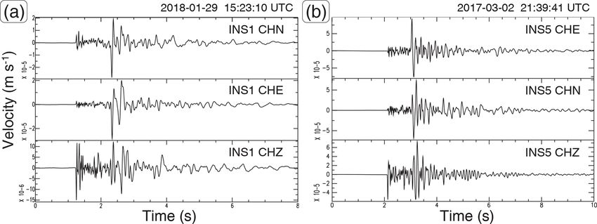
528                                                                                 T. A. Stabile et al.: The INSIEME seismic network

Figure 7. Probabilistic power spectral densities (PPSDs) computed for each component of the station INS1 (a, b, c), with a sensor installed
at 50 m depth, and the station INSX (d, e, f), with a sensor installed at the surface. The colour palettes on the right indicate the probability
(in percentage) of having a certain noise level. The two grey curves in each panel indicate the new high- and low-noise models, respectively,
obtained by Peterson (1993). Below all PPSD panels the data basis is visualized: the top row is coloured in green for available data and in
red (not in this case) for eventual gaps in streams. The bottom row is coloured in blue if the single PSD measurement is included in the PPSD
computation. Periods above 20 s are highlighted in grey because in such a period range it is not possible to compare the PPSD of the two
stations (only the sensor of INS1 stations has a flat response up to 120 s).

INS5 with respect to station INS6 before 22 March 2017 is                 different depths of the sensor are shown in the Supplement
very clear, particularly for the two horizontal components,               (Figs. S1–S8), which also shows with black curves the 5th,
but the noise levels are comparable in the period of time                 the 55th (median), and the 95th percentiles. The PPSD func-
when both stations have their sensors installed at depth. Af-             tions computed over the whole period of operation of the net-
ter 22 March 2017 it is possible to observe that the high-                work confirm that the noise level is more widespread when
frequency (> 1 Hz) day–night succession of INS5 station is                the sensor is installed on the surface with respect to the in-
a little bit more pronounced than the day–night succession of             stallation in shallow boreholes (see 95th percentile curves in
INS6 station because the former is closer to the urban area               Figs. S1–S8) and that there is no significant reduction of the
of Sarconi town than the latter. Finally, it is interesting to ob-        noise level for installation of sensors between 6 and 50 m
serve, as expected, the increase in the microseismic noise in             depth.
the range 4–8 s generated by the sea activity during storms
(e.g. in the period 6–9 March 2017 as effects of a strong mis-
                                                                          3.2    Data quality in terms of local ground effects
tral event in the Tyrrhenian Sea); this phenomenon is masked
by the high noise level when the sensors are placed on the                According to Havskov et al. (2012), local seismic amplifica-
surface.                                                                  tions due to sensor installation on soft ground can greatly af-
   Finally, for a comprehensive analysis of the noise level               fect spectral analyses of low and moderate earthquakes; the
at the different investigated depths, we computed the PPSD                use of broadband recordings may become difficult, and the
over the entire period of operation of the network for all                short period signals may be unrepresentative. The absence
components of all stations. Figure 10 displays the median                 of meaningful site effects was assessed beforehand for prop-
values of PPSD for the vertical components (channel CHZ)                  erly choosing the future locations of each seismic station of
of sensors installed at different depths and locations. It is             the INSIEME network. In order to check the validity of our
worth noting that for frequencies above 1.5 Hz (periods be-               choice and the quality of seismic signals, a further assess-
low 0.6 s) the median curves obtained for sensors installed               ment of the negligible site effect on recorded data has been
on the surface (black lines in Fig. 10) are generally 10 dB               carried out.
higher than the median curves obtained for sensors installed                 To this purpose earthquake data have been selected
at depth (blue, green, and red curves in Fig. 10). The PPSDs              from the preliminary catalogue of HAV seismicity
computed for each component of each individual station at                 (https://doi.org/10.5281/zenodo.3632419; Stabile et al.,

Earth Syst. Sci. Data, 12, 519–538, 2020                                                     www.earth-syst-sci-data.net/12/519/2020/
T. A. Stabile et al.: The INSIEME seismic network 529
Figure 8. Same type of comparison as Fig. 7 but among stations INS1 (sensor installed at 50 m depth), INS2 and INS4 (respective sensors
both installed at 6 m depth).
2020). With the aim to have more accurate locations, In addition to earthquake data, 5 h of seismic noise data
the events have been relocated by means of NonLinLoc (SN hereinafter) were extracted in the time window 09:00–
code (Lomax et al., 2000) in a 3-D velocity model of the 14:00 UTC of 26 November 2018.
area (Serlenga and Stabile, 2019), allowing us to better In order to assess the presence of possible local ground
distinguish three different categories of seismic events. effects at the sites where the stations were installed, the
selected data were analysed by applying the horizontal-to-
a. The first is injection-induced earthquakes (IIEs here- vertical spectral ratio technique (HVSR; Nakamura, 1989),
inafter), whose epicentres belong to the cluster B lo- both to earthquakes and to noise data (HVNSR, where the
cated NE of the Pertusillo lake and close to the CM2 in- letter “N” stands for “noise”).
jection well (see Fig. 1). We also increased the number For this purpose, each component of earthquake data was
of IIEs by using a template-matching algorithm based cut in time windows which allowed us to discard as much as
on the cross-correlation processing for single station possible the pre- and post-signal noise. For IIE, RIE, and LE
data proposed by Roberts et al. (1989). In this way we data we chose 8, 16, and 32 s wide time windows, respec-
were able to use 164 injection-induced earthquakes. tively, with a corresponding minimum frequency of 0.125,
0.0625, and 0.03125 Hz. In order to have reliable estimates
b. The second is reservoir-induced earthquakes (RIEs the spectra were evaluated starting from 10 times the respec-
hereinafter), belonging to the cluster A located SW of tive minimum frequency (i.e. 1.25, 0.625, and 0.3125 Hz).
the lake (see Fig. 1), for a total number of 56 events. The difference in the selected time windows is related to the
dissimilar durations of recorded signals of each category of
earthquakes. Before computing the fast Fourier transform,
c. The third is local earthquakes (LEs hereinafter) located
the mean and the trend were removed from the time series
in the HAV. In particular, only events with a magnitude
and signals belonging to any data category were tapered by
greater than 1.5 were selected, for a total number of 33
applying a Tukey window with 5 % bandwidth. Then, the
events.
www.earth-syst-sci-data.net/12/519/2020/ Earth Syst. Sci. Data, 12, 519–538, 2020530 T. A. Stabile et al.: The INSIEME seismic network
Figure 9. Spectrograms of each component of stations INS5 (a, b, c) and INS6 (c, d, e) computed over continuous data streams of 41 d (from
2 March to 11 April 2017). The sensor of station INS5 was installed at 6 m depth for the whole period of observation whereas the sensor of
station INS6 was first installed on the surface and then moved at 6 m depth on 22 March 2017.
computed spectra were smoothed by means of the Konno–
Ohmachi function (Konno and Ohmachi, 1998), with a band-
width coefficient equal to 40. The HVSR for each earthquake
was retrieved from the arithmetic mean of the horizontal am-
plitude spectral components (EW and NS) over the vertical
amplitude spectral component (Z) of the acquired signal, that
is
EW + NS
HVSR = . (2)
2Z
Finally, the average HVSR for each station and earthquake
category was computed, along with the ±1σ (1 standard de-
viation). The choice of performing such an analysis on dif-
ferent types of earthquakes, characterized by a heterogeneous
location in space, was related to look for possible source and
Figure 10. Median values of PPSD computed for the vertical com- directivity effects on the consequent HVSR measurements.
ponents (channel CHZ) of sensors installed at different depths and The 5 h long SN data, on the other hand, were cut in
locations over the entire period of operation of the INSIEME seis-
130 s wide non-overlapping time windows, which spanned
mic network. Black curves are the median values of PPSD com-
the total temporal extension of the recording, providing a
puted when sensors were installed on the surface; blue, green, and
red curves refer to sensors installed at 6, 14, and 50 m depth, respec- total number of 138 signals with a spectral resolution of
tively. For sensors with a flat response up to 20 s, the median curves 0.007 Hz. The retrieved time series were processed in an
are plotted up to that period. The two grey curves indicate the new analogous way to the one described before for earthquake
high- and low-noise models. data by means of the Geopsy software (Geopsy project;
http://www.geopsy.org, last access: January 2020). For each
time window and station, the HVNSR was retrieved, taking
into account that the horizontal spectrum was computed as
Earth Syst. Sci. Data, 12, 519–538, 2020 www.earth-syst-sci-data.net/12/519/2020/T. A. Stabile et al.: The INSIEME seismic network 531
Figure 11. HVSR and HVNSR curves computed at all the INSIEME network seismic stations. For each dataset, the number of used
earthquakes and the hours of seismic noise are indicated. The solid coloured lines represent the average HVSR and HVNSR curves, whereas
the dashed lines identify the ±1σ standard deviations.
the squared average of the two horizontal (EW and NS) com- indeed, the retrieved HVNSR curves are flatter than HVSR
ponents: ones.
In Fig. 11 we observe very low site amplifications, ex-
s
cept for the INS5 seismic station, where a relevant peak
EW2 + NS2
H= . (3) at about 3.5 Hz can be noticed and for INS6 whose HVSR
2 function has a slight amplification between 0.8 and 3.0 Hz.
Some detailed considerations of the results related to station
Finally, the average HVNSR of each station was computed, INS1 must be taken. Previous analyses performed at the same
along with the ±1σ . site with ambient noise and earthquake data, by using both
The retrieved HVSR and HVNSR are represented in a seismometer and an accelerometer located at the surface,
Fig. 11. We can assert that most of the stations are charac- and with geological and geophysical (electrical resistivity to-
terized by an almost flat H /V curve, independently of the mography) surveys allowed us to approximately estimate the
adopted dataset. Furthermore, we separately verified that the depth of the bedrock at about 50 m (Giocoli et al., 2015). In-
choice of an arithmetic mean or a squared average of the two deed, an amplitude peak between 2 and 3 Hz in the retrieved
horizontal components is almost completely irrelevant to the H /V curves was clearly observable. By looking at Fig. 11,
consequent HVSR or HVNSR measurements. The arithmetic this peak is no longer present, confirming that the installa-
average adopted for earthquake data analysis allowed us to tion of INS1 at 50 m depth allowed us to reach a more rigid
equally weight possible amplitude peaks related to directivity (higher acoustic impedance) layer; in addition, during perfo-
and azimuthal effects in the HVSR computation. On the other ration operations, a sharp lithological change from alluvial
hand, the squared average, which generally overestimates the deposits to the Gorgoglione Formation was clearly observed
arithmetic average and which was adopted for analysing the at that depth. At INS1 seismic station, the low-amplitude
ambient noise data, did not produce higher amplitude peaks:
www.earth-syst-sci-data.net/12/519/2020/ Earth Syst. Sci. Data, 12, 519–538, 2020532 T. A. Stabile et al.: The INSIEME seismic network
peaks at about 4–5, 9, and 11 Hz are observed in HVSR (Ml = 1.4; lat 40.3182◦ N, long 15.9842◦ E; depth =
curves but not in the HVNSR one. We might interpret these 3.50 km; from https://doi.org/10.5281/zenodo.3632419,
differences as the effect of the down-going earthquake wave Stabile et al., 2020). Most detected IIEs have a magni-
field. tude lower than or equal to 1; only two of them are char-
acterized by local magnitude of Ml = 1.1 and Ml = 1.4.
Depending on the earthquake energy, the number of sta-
3.3 Induced microearthquakes, local earthquakes, and
tions that recorded the seismic signals changes from a
teleseismic events
minimum of three for the lowest magnitude event up to
The continuous data acquisition by the INSIEME seismic 16, also taking into account stations belonging to the
network allowed us to manually detect, by a visual inspec- virtual seismic network. The waveforms, usually, have
tion of recordings through the SefraN tool, a total number a duration of less than 7 s at the closest station (INS1),
of 852 local natural and induced earthquakes between and the highest peak ground velocity amplitude (PGV)
September 2016 and March 2019. Then, these were pre- measured at that station is about 0.04 mm s−1 for the
liminarily located (https://doi.org/10.5281/zenodo.3632419; strongest IIE of the catalogue (Fig. 12a).
Stabile et al., 2020) using the 1-D velocity model by
Improta et al. (2017) and Hypo71 algorithm (Lee and b. RIE. A total of 117 reservoir-induced seismic events
Lahr, 1972) embedded in SeisComP3, allowing us to have were manually picked and located, in the range 0 ≤
an initial distinction of the three different categories of Ml ≤ 1.8. The P-wave arrivals are usually first detected
seismic events already introduced in the previous section at the INS5, INS6, or INS7 seismic stations, depending
(Sect. 3.2): IIE, RIE, and LE. In order to better locate on the earthquake location: indeed, such induced events
local events outside the INSIEME network, we build belong to a wider cluster than IIEs and therefore they
a virtual seismic network composed of 11 seismic sta- are more broadly distributed in the southwestern part of
tions of the Italian National Seismic Network (FDSN the seismic network (cluster A in Fig. 1). Their average
codes: IV, https://doi.org/10.13127/SD/X0FXnH7QfY, depth is about 4.5 km and the maximum recorded local
INGV Seismological Data Centre, 2006; MN, magnitude is Ml = 1.8, related to an event that occurred
https://doi.org/10.13127/SD/fBBBtDtd6q, MedNet Project on 2 March 2017 at 21:39:41 UTC (Fig. 12b), located at
Partner Institutions, 1990) managed by the Italian National about 1.9 km epicentral distance from the INS5 station
Institute of Geophysics and Volcanology (INGV), seven (Ml = 1.8; lat 40.2723◦ N, long 15.8840◦ E; depth =
stations belonging to the Irpinia Seismic Network (Weber et 4.51 km; from https://doi.org/10.5281/zenodo.3632419,
al., 2007; Stabile et al., 2013; FDSN code: IX), and MARCO Stabile et al., 2020). Because of the proximity of the sta-
station belonging to the GEOFON network (FDSN code: tions around this seismicity cluster, RIE earthquakes, in
GE, https://doi.org/10.14470/TR560404, GEOFON Data a way similar to IIE, are also characterized by a differ-
Centre, 1993), the last installed south of Tramutola town ence between S- and P-wave arrival times of about 1 s
in the framework of a joint scientific cooperation between at the closest station to the epicentre and short duration,
GFZ Potsdam and CNR-IMAA institutes; all the stations of less than 8 s (e.g. see Fig. 12b). The recorded seismic
the virtual network are located within about 60 km distance event with the lowest magnitude was detected by seven
from the centre of the INSIEME network. stations, whereas the strongest earthquake was recorded
Here we report the main inferred features for each earth- by 12 stations. Finally, the highest peak ground velocity
quake category (IIE, RIE, and LE), in terms of both seismic amplitude recorded up to now for this earthquake cate-
signal properties and hypocentral locations: gory is about 0.08 mm s−1 (Fig. 12b).
a. IIE. A total of 43 injection-induced seismic events were c. LE. A total of 692 local natural earthquakes were man-
manually picked and located. These were identified ually picked and located. The main difference with re-
because they belong to the seismicity cluster induced spect to the IIE and RIE is that they are not clus-
by fluid-injection operations at the CM2 well (clus- tered; they are characterized by a widespread dis-
ter B in Fig. 1). The first recording station of such tribution in the investigated area, and their average
events is INS1, which is the closest receiver, with sig- hypocentral depth of about 10 km is more similar to
nals characterized by a difference between the arrival the typical depth of Apennines crustal earthquakes.
times of S and P waves of about 1 s. The average Most recorded LEs are characterized by a local mag-
depth retrieved from preliminary event location anal- nitude < 2: only 39 seismic events out of 692 have
yses is about 4.5 km and the maximum recorded lo- a greater magnitude. Four earthquakes with a mag-
cal magnitude is Ml = 1.4, related to an induced event nitude greater than 3, included in a radius of about
that occurred on 29 January 2018 at 15:23:10 UTC 40 km from the centre of the INSIEME seismic net-
(Fig. 12a), located at about 1.4 km epicentral distance work, have been recorded. The strongest event close
from the INS1 station with a focal depth of about 3.0 km to the INSIEME network (epicentral distance of 16 km
Earth Syst. Sci. Data, 12, 519–538, 2020 www.earth-syst-sci-data.net/12/519/2020/T. A. Stabile et al.: The INSIEME seismic network 533
Figure 12. (a) The largest injection induced event (Ml = 1.4; lat 40.3182◦ N, long 15.9842◦ E; depth = 3.50 km) recorded by the INS1
seismic station at 1.4 km epicentral distance, and (b) the largest reservoir induced event (Ml = 1.8; lat 40.2723◦ N, long 15.8840◦ E; depth
= 4.51 km) recorded by the INS5 seismic station at 1.9 km epicentral distance. At the top of the figures the seismic event origin time is
reported. For station INS1 the original horizontal components were rotated anticlockwise by an angle of 307.8◦ with respect to the north,
according to the computations described in detail in Sect. 2.2. A ts –tp of about 1 s can be clearly noticed for both the injection and the
reservoir induced events at the correspondent closest station.
from INS5 and INS6 stations) is a Mw = 3.8 earth- 4 Data availability
quake (from http://cnt.rm.ingv.it/event/17474201, last
access: January 2020). The highest peak ground ve-
locity amplitude of more than 3 mm s−1 was recorded The INSIEME network has been registered at the In-
at MTSN station, managed by INGV, which was the ternational Federation of Digital Seismograph Networks
closest station located at 5 km epicentral distance. The (FDSN), which assigned the network code 3F (2016–2019)
earthquake was recorded by the whole INSIEME seis- (https://doi.org/10.7914/SN/3F_2016; Stabile and the IN-
mic network, as well as by all the stations of the virtual SIEME Team, 2016). Open-access policy on these data has
network that were in operation that day (event Ml = 4.0; been adopted under the license CC BY 4.0. Continuous seis-
lat 40.3040◦ N, long 15.7200◦ E; depth = 12.10 km re- mic data are available at IRIS DMC from 1 April 2016 to
ported in https://doi.org/10.5281/zenodo.3632419; Sta- 23 March 2019 (see Fig. 4 illustrating the availability of
bile et al., 2020); in Fig. 13 the vertical components of seismic data for all stations of the network). From IRIS
the 18 stations that have recorded the earthquake are dis- DMC FDSN Web Services (https://service.iris.edu, last ac-
played. cess: January 2020) it is possible to download the standard
StationXML file (service interface “station”) of each station
Concerning teleseismic events, the INSIEME network was of the network which reports comprehensive information of
able to record the most energetic earthquakes that occurred the station including the instrument response, the time se-
worldwide in the period in which the analyses have been car- ries data in miniSEED and other formats (service interface
ried out. In Fig. 14, the recordings at INS1 station of seismic “datalesect”), and the time series data availability (service
waves generated by the Mw = 7.6 Chile earthquake of 25 De- interface “availability”).
cember 2016 are shown. We specifically choose to display The events preliminarily located with the Origin Lo-
the waveforms at INS1 station since it was installed at 50 m cator Viewer (scolv) tool of the SeisComP3 software
depth and it is a 120 s instrument: these elements allowed us are available in the “Preliminary catalogue of High
to clearly see the most important seismic phases generated Agri Valley seismicity (southern Italy) recorded by
by the earthquake and by the effects of propagation inside the temporary INSIEME network” CSV file (available
the Earth. Their theoretical arrival times were computed by at https://doi.org/10.5281/zenodo.3632419; Stabile et al.,
means of SeisGram2k software (Lomax, 2008), which uses 2020). The KMZ file “INSIEME-network.kmz” (Keyhole
the Preliminary Reference Earth Model (PREM) published Markup language Zipped, which can be viewed using Google
by Dziewonski and Anderson (1981). In addition to different Earth), provided in the Supplement, is an interactive exten-
seismic phases, in Fig. 14 we are able to observe the dis- sion of Fig. 1 also showing the layout of the virtual network
persive character of surface waves, with lower frequencies, used to preliminarily locate all the events.
travelling deeper in the Earth and, therefore, faster, arriving Following the end of the SIR-MIUR INSIEME project
at the INS1 station before the higher frequencies. (23 March 2019), the temporary INSIEME network is go-
ing to be updated as a permanent open-access seismic net-
work under the license CC BY 4.0; therefore, acquired data
after 23 March 2019 will be available from the permanent
www.earth-syst-sci-data.net/12/519/2020/ Earth Syst. Sci. Data, 12, 519–538, 2020You can also read