ENGINEERING GUIDELINES FOR THE EVALUATION OF HYDROPOWER PROJECTS - CHAPTER 13 - EVALUATION OF EARTHQUAKE GROUND MOTIONS
←
→
Page content transcription
If your browser does not render page correctly, please read the page content below
ENGINEERING GUIDELINES FOR THE
  EVALUATION OF HYDROPOWER
          PROJECTS

   CHAPTER 13 – EVALUATION OF
  EARTHQUAKE GROUND MOTIONS

                MAY 30, 2018
     FEDERAL ENERGY REGULATORY COMMISSION
                 888 First Street, NC
                Washington, DC 20426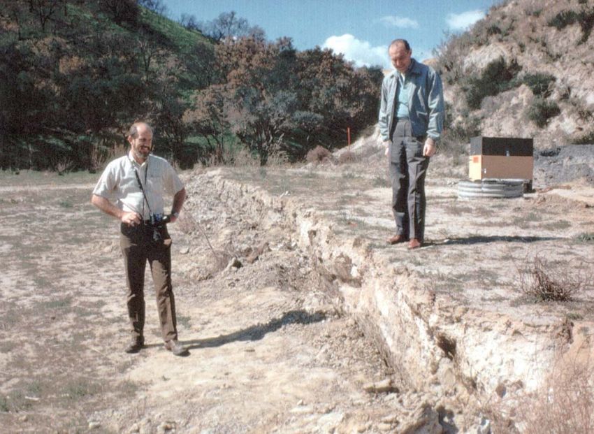
EVALUATION OF EARTHQUAKE GROUND
            MOTIONS

                            Prepared by

    I. M. Idriss, Professor Emeritus, Univ. of California at Davis
          Consulting Geotechnical Engineer, Santa Fe, NM
                       e-mail: imidriss@aol.com

             Ralph J. Archuleta, Professor Emeritus
      Department of Earth Science & Earth Research Institute
            University of California at Santa Barbara
               e-mail: ralph.archuleta@ucsb.edu

                               and
                    Norman A. Abrahamson
       Consulting Engineering Seismologist, Piedmont, CA
     e-mail: naa3@earthlink.net & abrahamson@berkeley.edu

                            Prepared for

              Division of Dam Safety and Inspections
                     Office of Energy Projects
          Federal Energy Regulatory Commission (FERC)
                       888 First Street, N.E.
                     Washington, D.C. 20426

                           May 30, 2018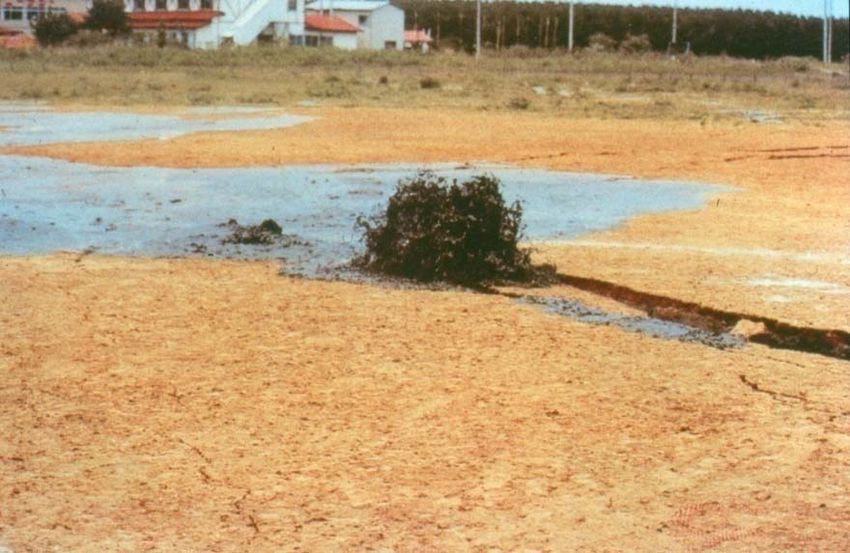
TABLE OF CONTENTS

                                                                                                          Page
1.0        INTRODUCTION                                                                                    1

           1.1 Introductory Comments                                                                        1

           1.2 Organization of the Report                                                                   2

2.0        EARTHQUAKE HAZARDS AND CONSEQUENCES                                                              2

           2.1 General                                                                                      2

           2.2 Fault Rupture                                                                                2

           2.3 Soil Failure                                                                                 5

           2.4 Seiches                                                                                      11

3.0        GEOLOGIC AND SEISMOLOGIC CONSIDERATIONS                                                          12

           3.1 Historical Seismicity                                                                        12

           3.2 Seismographic Record                                                                         12

           3.3 Geologic Studies                                                                             13

           3.4 Earthquake Recurrence Models                                                                 22

           3.5 Other Seismic Sources                                                                        27

4.0        SEISMIC HAZARD EVALUATION                                                                        28

           4.1 Deterministic Seismic Hazard Evaluation                                                      28

           4.2 Probabilistic Seismic Hazard Evaluation                                                      30

5.0        ESTIMATION OF EARTHQUAKE GROUND MOTIONS AT A ROCK                                                32
           OUTCROP

           5.1 General                                                                                      32

           5.2 Empirical Procedures                                                                         33

           5.3 Analytical Procedures                                                                        33

6.0        GUIDELINES                                                                                       34

           6.1 Required Geologic Studies                                                                    34

Evaluation of Earthquake Ground Motions               Page i                                         May 30, 2018
For The Federal Energy Regulatory Commission (FERC)            by I. M. Idriss, R. J. Archuleta and N. A. Abrahamson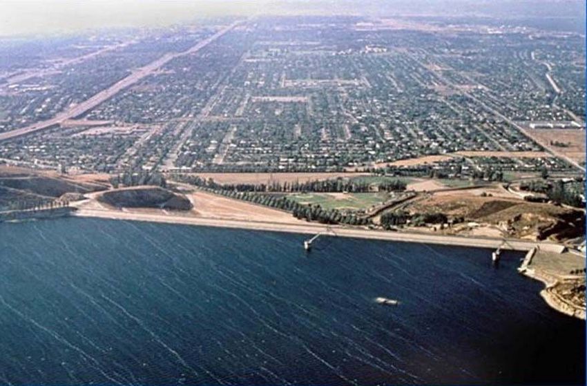
6.2 Required Seismologic Studies                                                                  34

           6.3 Deterministic Development of Earthquake Ground Motions                                        35

           6.4 Probabilistic Development of Earthquake Ground Motions                                        35

           6.5 Minimum Required Parameters for Controlling Events(s)                                         36

7.0        REFERENCES                                                                                        37

APPENDIX A: METHODS FOR ESTIMATING MAXIMUM EARTHQUAKE MAGNITUDE
APPENDIX B: SELECTION OF APPROPRIATE PERCENTILE GROUND MOTION LEVEL
            IN A DETERMINISTIC SEISMIC HAZARD EVALUATION
APPENDIX C: EXAMPLES – PROBABILISTIC SEISMIC HAZARD ANALYSIS
APPENDIX D: EARTHQUAKE GROUND MOTIONS MODELS
APPENDIX E: ANALYTICAL SIMULATIONS TO GENERATE ACCELEROGRAMS AT A
            ROCK SITE
APPENDIX F: SELECTION OF ACCELEROGRAMS FOR SEISMIC ANALYSIS

Evaluation of Earthquake Ground Motions               Page ii                                         May 30, 2018
For The Federal Energy Regulatory Commission (FERC)             by I. M. Idriss, R. J. Archuleta and N. A. Abrahamson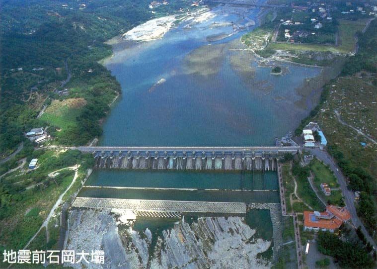
LIST OF TABLES

Table 1            Examples of Slip Rates

                                             LIST OF FIGURES

Figure 2-1         Horizontal (Strike-Slip) Fault Offset of the Imperial Fault in 1940 across the All-
                   America Canal Caused by the 1940 El Centro Earthquake

Figure 2-2         Red Canyon Fault Scarp East of Blarney Stone Ranch Caused by the 1959
                   Montana Earthquake

Figure 2-3         Fault Rupture of San Fernando Fault in 1971; the late Professor H. Bolton Seed
                   was Standing on the Hanging Wall and Lloyd Cluff was Standing on the Footwall
                   (Photograph: Courtesy of Professor Clarence Allen)

Figure 2-4         View of Dam in Taiwan Prior to the Occurrence of the 1999 Chi Chi Earthquake

Figure 2-5         View of Dam after the 1999 Chi-Chi Earthquake Showing Damage to Portion of
                   Dam due to Fault Rupture

Figure 2-6         View of fault rupture adjacent to bridge downstream of the dam, shown in Figures
                   2-4 and 2-5, resulting in formation of falls in river and damage to bridge structure.

Figure 2-7         Aerial View of Austrian Dam

Figure 2-8         Longitudinal and Transverse Cracks in Austrian Dam Caused by Shaking during
                   the 1989 Loma Prieta Earthquake (after Vrymoed & Lam, 1991)

Figure 2-9         Vertical and Horizontal Displacements, in feet, of the Crest of Austrian Dam at
                   Station 6+00 (after Vrymoed & Lam, 1991)

Figure 2-10        Vertical and Horizontal Displacements, in feet, of the Crest of Austrian Dam at
                   Station 2+50 (after Vrymoed & Lam, 1991)

Figure 2-12        San Fernando Dam Complex shortly after the Occurrence of the 1971 San
                   Fernando Earthquake

Figure 2-13        View of Upper San Fernando Dam Showing Horizontal and Vertical Deformations
                   and Cracks in the Upstream Face of the Dam

Figure 2-14        Close-up View of Cracks in the Upstream Face of Upper San Fernando Dam

Figure 2-15        Aerial View Lower San Fernando Dam before the occurrence of the 1971 San
                   Fernando Earthquake showing the Extensive Number of Residences that Would
                   Have Been Affected by a Breach of the Dam (Photograph: Courtesy of David
                   Gutierrez)

Figure 2-16        Photograph of the Lower San Fernando Dam taken a few Hours after the
                   Occurrence of the 1971 San Fernando Earthquake
Evaluation of Earthquake Ground Motions               Page iii                                         May 30, 2018
For The Federal Energy Regulatory Commission (FERC)              by I. M. Idriss, R. J. Archuleta and N. A. Abrahamson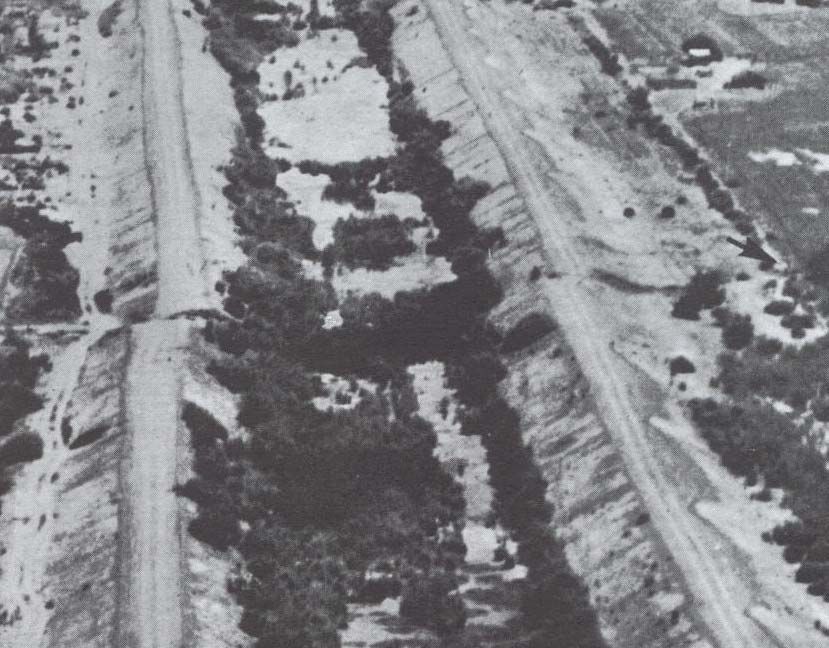
Figure 2-17        Photograph of the Lower San Fernando Dam taken after Partial Emptying the
                   Reservoir Showing the Extent of Lateral Flow of the Upstream Shell and Crest of
                   the Dam

Figure 2-18        View of the Madison River Slide from Earthquake Lake Side; Slide occurred
                   during the 1959 Montana Earthquake

Figure 3-1         Aerial View of San Andreas Fault near Palmdale Reservoir in Southern
                   California (From Richter, 1958)

Figure 3-2         Log of Trench across Fault on which the 1968 Borrego Mountain, California,
                   Earthquake Occurred (From Clark et al., 1972)

Figure 3-3         Schematic Illustration of Four Types of Faults

Figure 3-4         Relation between Moment Magnitude and Various Magnitude Scales (after
                   Heaton et al., 1982)

Figure 3-5         Relationship between M and mbLg

Figure 3-6         Location Map of the South-Central Segment of the San Andreas Fault

Figure 3-7         Plot of Instrumental Seismicity Data for the Period of 1900 – 1980 Along the
                   South-Central Segment of the San Andreas Fault; the Box in the Figure
                   Represents Range of Recurrence for M = 7.5 – 8, Based on Geologic Data (from
                   Schwartz and Coppersmith, 1984)

Figure 3-8         Characteristic Earthquake Recurrence Model for South Central Segment of San
                   Andreas Fault

Evaluation of Earthquake Ground Motions               Page iv                                         May 30, 2018
For The Federal Energy Regulatory Commission (FERC)             by I. M. Idriss, R. J. Archuleta and N. A. Abrahamson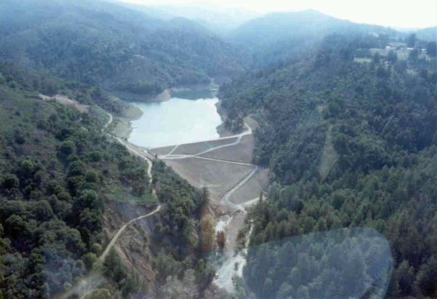
EVALUATION OF EARTHQUAKE GROUND MOTIONS
                                                       by

                   I. M. Idriss, Ralph J. Archuleta and Norman A. Abrahamson

1.0    INTRODUCTION

1.1    Introductory Comments

The Division of Dam Safety and Inspections of the Office of Energy Projects at the Federal Energy
Regulatory Commission (FERC) is responsible for the safety of power-generating stations
throughout the USA. This responsibility includes concern with the effects of earthquakes at these
stations, which typically include dams and appurtenant structures. Accordingly, FERC requested
that the writers prepare this document on "Evaluation of Earthquake Ground Motions" that contains
the main elements that could be utilized by FERC to establish "Seismic Design Criteria" for all
facilities under its jurisdiction.

The purpose of seismic design criteria is to provide guidelines and procedures for obtaining
earthquake ground motion parameters for use in evaluating the seismic response of a given structure
or facility. Presently, there are three ways by which the earthquake ground motion parameters can
be ascertained: (i) use of local building codes; (ii) conducting a deterministic seismic hazard
analysis (DSHA); and (iii) conducting a probabilistic seismic hazard analysis (PSHA). Typically,
local building codes are intended to mitigate collapse of buildings and loss of life, and do not apply
to structures covered in this document. Both deterministic and probabilistic seismic hazard
analyses and evaluations are covered in this document.

The earthquake ground motion parameters discussed in this document pertain to a "rock outcrop".
Thus, these parameters are intended for use as input to an analytical model that would include the
structure under consideration, e.g., a dam-foundation system. Any effects of local site conditions
on earthquake ground motions would then be explicitly accounted for in the analyses. Accordingly,
the effects of local site conditions on earthquake ground motions, which can be very significant,
are not addressed in this document.

To provide the needed basis for estimating earthquake ground motion parameters at a particular
"rock outcrop", it is necessary to incorporate the appropriate geologic and seismologic input and to
utilize the most relevant available procedures for estimating these parameters. The remaining pages
of this document cover these aspects and the appendices include more details regarding specific
aspects of the seismic hazard evaluation procedures.

Evaluation of Earthquake Ground Motions               Page 1                                         May 30, 2018
For The Federal Energy Regulatory Commission (FERC)            by I. M. Idriss, R. J. Archuleta and N. A. Abrahamson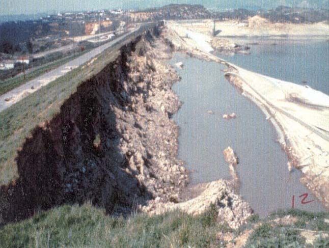
1.2    Organization of the Report

In addition to this introductory section, the report includes six sections and six appendices and a
list of references. The appendices are structured so that they can be updated periodically as new
developments and publications pertinent to each appendix become available.

2.0    EARTHQUAKE HAZARDS AND CONSEQUENCES

2.1    General

This section is included in this document merely to highlight why seismic hazards can be very
important to facilities under the jurisdiction of FERC. Hazards that may affect such facilities
include fault rupture, soil failure, and seiches. Other hazards, such as tsunamis, are not discussed
in this document because all of the facilities under FERC's jurisdiction are inland and are unlikely
to be affected by tsunamis.

2.2    Fault Rupture

Fault rupture is a hazard that must be dealt with whenever a fault traverses a dam site. The potential
for the presence of a fault, or fault traces, at a particular site should be fully investigated to assess
the location, orientation, type, sense of movement … etc.

Typical examples of fault rupturing in historic earthquakes are presented in Figures 2-1 through 2-
6. Possible approaches to allowing for the effects of fault rupture on embankment dams are offered,
for example, in Sherard et al. (1974) and other regulatory documents. The exact method that the
licensee uses must be appropriately documented.

Figure 2-1 Horizontal (Strike-Slip) fault offset of the Imperial Fault in 1940 across the All-
America Canal caused by the 1940 El Centro earthquake.

Evaluation of Earthquake Ground Motions               Page 2                                         May 30, 2018
For The Federal Energy Regulatory Commission (FERC)            by I. M. Idriss, R. J. Archuleta and N. A. Abrahamson
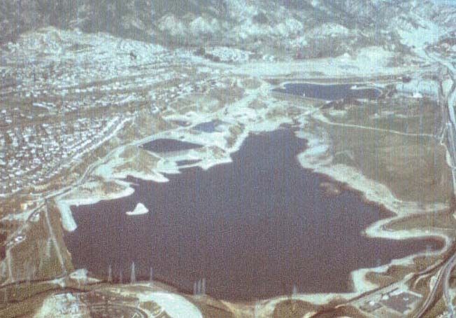
Figure 2-2 Red Canyon Fault Scarp East of Blarney Stone Ranch Caused by the 1959 Montana
Earthquake.

Figure 2-3 Fault Rupture of San Fernando Fault in 1971; the late Professor H. Bolton Seed was
standing on the Hanging Wall and Lloyd Cluff was standing on the Footwall.
                      (Photograph: Courtesy of Professor Clarence Allen)

Evaluation of Earthquake Ground Motions               Page 3                                         May 30, 2018
For The Federal Energy Regulatory Commission (FERC)            by I. M. Idriss, R. J. Archuleta and N. A. Abrahamson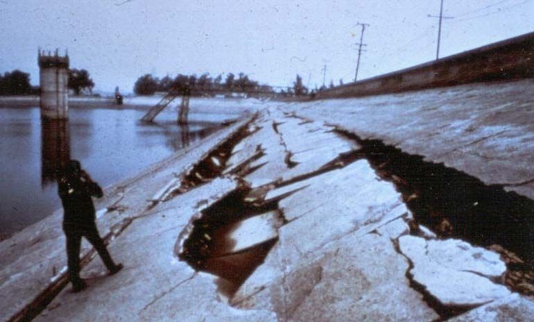
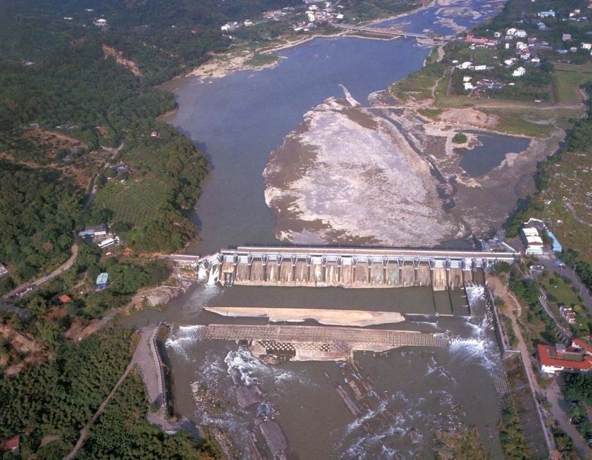
Figure 2-4 View of dam in Taiwan prior to the occurrence of the 1999 Chi-Chi earthquake.

Figure 2-5 View of dam after the 1999 Chi-Chi Earthquake showing damage to portion of the
dam due to fault rupture.

Evaluation of Earthquake Ground Motions               Page 4                                         May 30, 2018
For The Federal Energy Regulatory Commission (FERC)            by I. M. Idriss, R. J. Archuleta and N. A. Abrahamson
Figure 2-6 View of fault rupture adjacent to bridge downstream of the dam, shown in Figures 2-4
and 2-5, resulting in formation of falls in river and damage to bridge structure.
2.3 Soil Failure
2.3.1 Foundation and/or Embankment Soils
Strong earthquake ground motions can induce high pore water pressures and/or high strains in these
soils that could have serious consequences, including:
Settlements, which are mostly abrupt and non-uniform and often lead to longitudinal as
well as transverse cracks.
Loss of bearing support.
Floatation of buried structures, such as underground tanks or pipes.
Increased lateral pressures against retaining structures.
Lateral spreads (limited lateral movements).
Lateral flows (extensive lateral movements).
Examples of settlements leading to cracks coupled with limited lateral movements are illustrated
by the performance of Austrian Dam in California during the 1989 Loma Prieta earthquake as
shown in Figures 2-7 through 2-10.
Evaluation of Earthquake Ground Motions Page 5 May 30, 2018
For The Federal Energy Regulatory Commission (FERC) by I. M. Idriss, R. J. Archuleta and N. A. AbrahamsonFigure 2-7 Aerial view of Austrian Dam. (Photograph: Courtesy of David Gutierrez). Figure 2-8 Longitudinal and transverse cracks in Austrian Dam caused by shaking during the 1989 Loma Prieta earthquake (after Vrymoed & Lam, 1991). Evaluation of Earthquake Ground Motions Page 6 May 30, 2018 For The Federal Energy Regulatory Commission (FERC) by I. M. Idriss, R. J. Archuleta and N. A. Abrahamson
Figure 2-9 Vertical and horizontal displacements, in feet, of the crest of Austrian Dam at Station
6+00 (after Vrymoed & Lam, 1991).

Figure 2-10 Vertical and horizontal Displacements, in feet, of the crest of Austrian Dam at
Station 2+50 (after Vrymoed & Lam, 1991).

Among the consequences of increased pore water pressure is the possibility of triggering
liquefaction in cohesionless soils, such as sands, silty sands and very low plasticity or non-plastic
sandy silt. An example of liquefaction "in progress" is shown in Figure 2-11 – a view captured
during the magnitude 7½ 1978 Miyagi-Ken-Oki earthquake in Japan.

Figure 2-11 Surface evidence of liquefaction triggered during the 1978 Miyagi-Ken-Oki
earthquake in Japan.

Evaluation of Earthquake Ground Motions               Page 7                                         May 30, 2018
For The Federal Energy Regulatory Commission (FERC)            by I. M. Idriss, R. J. Archuleta and N. A. Abrahamson
Examples of lateral spreads (limited lateral movements) and lateral flows (extensive lateral
movements) are provided by what happened to the Upper and Lower San Fernando Dams during
the 1971 San Fernando earthquake, as shown in Figure 2-12. Figures 2-13 and 2-14 provide more
details of the relatively limited lateral movements (lateral spreads) of the embankment of the Upper
San Fernando Dam.

                                                UPPER DAM

                           LOWER DAM

Figure 2-12 San Fernando Dam Complex shortly after the occurrence of the 1971 San Fernando
earthquake.

Figure 2-13 View of Upper San Fernando Dam showing horizontal and vertical deformations and
cracks in the upstream face of the dam.

Evaluation of Earthquake Ground Motions               Page 8                                         May 30, 2018
For The Federal Energy Regulatory Commission (FERC)            by I. M. Idriss, R. J. Archuleta and N. A. Abrahamson
Figure 2-14 Close-up View of Cracks in the Upstream Face of Upper San Fernando Dam. An aerial view of the Lower San Fernando Dam before the occurrence of the 1971 San Fernando earthquake is shown in Figure 2-15. The devastating effects of the earthquake on this dam are presented in Figures 2-16 and 2-17. Note that the lateral flows caused by the ground shaking were initiated because of the liquefaction of the soils in the upstream shell of the dam and the resulting loss of strength of these soils. Figure 2-15 Aerial view Lower San Fernando Dam before the occurrence of the 1971 San Fernando Earthquake showing the extensive number of residences that would have been affected by a breach of the dam (Photograph: Courtesy of David Gutierrez). Evaluation of Earthquake Ground Motions Page 9 May 30, 2018 For The Federal Energy Regulatory Commission (FERC) by I. M. Idriss, R. J. Archuleta and N. A. Abrahamson
Figure 2-16 Photograph of the Lower San Fernando Dam taken a few hours after the occurrence
of the 1971 San Fernando Earthquake.

Figure 2-17 Photograph of the Lower San Fernando Dam taken after partial emptying the
reservoir showing the extent of lateral flow of the upstream shell and crest of the dam.

Evaluation of Earthquake Ground Motions               Page 10                                         May 30, 2018
For The Federal Energy Regulatory Commission (FERC)             by I. M. Idriss, R. J. Archuleta and N. A. Abrahamson
2.3.2    Reservoir Rim

Landslides along the rim of the reservoir can be triggered by the ground shaking during an
earthquake. Such landslides could impact the body of dam negatively, e.g., blocking an intake
tower, generating a wave that may overtop the crest etc. An example of a landslide is the Madison
River Slide in the 1959 Montana earthquake shown in Figure 2-18.

Figure 2-18 View of the Madison River Slide from earthquake lake side; Slide occurred during
the 1959 Montana Earthquake. (from USGS 1964)

2.4     Seiches

A seiche is a standing wave in an enclosed or partly enclosed body of water. Seiches are normally
caused by earthquake activity, and can affect reservoirs, harbors, bays, lakes, rivers and canals. In
the majority of instances, earthquake-induced seiches do not occur close to the source of an
earthquake, but some distance away (possibly as far as 100s of kilometers). This is due to the fact
that earthquake seismic waves close to the source are richer in high frequencies, while those at
greater distances are of lower frequency content which can enhance the rhythmic movement in a
body of water. The biggest seiches develop when the period of the ground shaking matches the
period of oscillation of the water body.

In 1891, an earthquake near Port Angeles caused an eight-foot seiche in Lake Washington; such a
rise in reservoir level could result in overtopping if the free board is not sufficient at the time. The
1964 Alaska earthquake created seiches on 14 inland bodies of water in the state of Washington,
including Lake Union where several pleasure craft, houseboats and floats sustained some damage.

Inland areas, though not vulnerable to tsunamis, are vulnerable to seiches caused by earthquakes.
Additional vulnerabilities include water storage tanks, and containers of liquid hazardous materials
that are also affected by the rhythmic motion.
Evaluation of Earthquake Ground Motions               Page 11                                         May 30, 2018
For The Federal Energy Regulatory Commission (FERC)             by I. M. Idriss, R. J. Archuleta and N. A. Abrahamson
Seiches create a "sloshing" effect on bodies of water and liquids in containers. This primary effect
can cause damage to moored boats, piers and facilities close to the water. Secondary problems,
including landslides and floods, are related to accelerated water movements and elevated water
levels.

The above description was obtained from text available from the following web site:
https://earthquake.usgs.gov/learn/topics/seiche.php

3.0     GEOLOGIC AND SEISMOLOGIC CONSIDERATIONS

Earthquake ground motions at a particular site are estimated through a seismic hazard evaluation.
The geologic and seismologic inputs needed for completing a seismic hazard evaluation consist of
acquiring information regarding the following key elements:

      a. The seismic sources on which future earthquakes are likely to occur;

      b. The size of the possible earthquakes and the frequency with which an earthquake is likely
         to occur on each source; and

      c. The distance and orientation of each source with respect to the site.

This information is obtained from the following sources of data in the region in which the site is
located: (1) The historical seismicity record; (2) the seismographic, or instrumental, record of
earthquake activity in the region; and (3) the geologic history, especially within the past few
thousand to several hundred thousand years.

3.1     Historical Seismicity

A necessary first step in a seismic hazard evaluation is the compilation and documentation of the
historical seismicity record pertinent to the region in which the site is located. It is essential in
assessing this historical seismicity record that local sources of data (e.g., newspaper accounts,
manuscripts written about a specific earthquake, etc.) be critically reviewed and that conflicting
information be resolved. The historical seismicity record in the USA is relatively brief as it extends
only over the past 200 to 400 years. It may be noted, however, that a good deal of the available
historical records for many parts of the country have been compiled and can be accessed. It is also
important to note that much of the historic seismicity record relies heavily (if not exclusively) on
reports of felt ground motions or patterns of damage.

Important as the historical seismicity record is, however, it is not sufficient by itself to estimate the
future seismic activity in a region.

3.2     Seismographic Record

The seismographic, or instrumental, record in a region is also an important tool in a seismic hazard
evaluation. Instrumental records augment the historical records by providing quantitative data
(e.g., size, location, depth, mechanism, and time of occurrence of earthquakes) that are not available
from reports of felt ground motions or patterns of damage.

The seismographic record is available only since the year 1900 and, until recently, only from a
limited number of stations in selected areas worldwide. Significant increases in the number of
Evaluation of Earthquake Ground Motions               Page 12                                         May 30, 2018
For The Federal Energy Regulatory Commission (FERC)             by I. M. Idriss, R. J. Archuleta and N. A. Abrahamson
stations worldwide have been implemented in the past few years and it is expected that the usefulness of the seismographic record will continue to increase in the coming years. 3.3 Geologic Studies In many parts of the world, significant earthquake activity can be directly associated with specific faults. A major earthquake typically leaves a distinct geologic record that can be preserved for thousands, and possibly hundreds of thousands, of years. The faulting associated with an earthquake may displace soil and/or rock strata at shallow depths and may create a fault scarp that remains visible. An example of a fault scarp is shown in Figures 3-1 and 3-2. Figure 3-1 is an aerial view of the San Andreas Fault, and Figure 3-2 is the log of the trench across the fault on which the 1968 Borrego Mountain, California, earthquake occurred. The preserved geologic features along faults can be investigated by geologic and geophysical studies that may include: review of available literature, especially with regard to structural and tectonic history; interpretation of various types of imagery to identify regional structures; reconnaissance of the geology and geomorphology of the region; and the use of trenching, boreholes, age-dating and geophysical techniques. Figure 3-1 Aerial view of San Andreas Fault near Palmdale Reservoir in Southern California (From Richter, 1958). Evaluation of Earthquake Ground Motions Page 13 May 30, 2018 For The Federal Energy Regulatory Commission (FERC) by I. M. Idriss, R. J. Archuleta and N. A. Abrahamson
Figure 3-2 Log of Trench across fault on which the 1968 Borrego Mountain, California,
earthquake occurred (From Clark et al., 1972).

There are various types of faults, as shown in Figure 3-3. In a thrust (or a reverse) fault, the offset
is along an inclined plane and occurs in response to a compressive tectonic strain environment as
shown in Figure 3-3a; examples of major earthquakes on such faults are the 1952 Kern County and
the 1971 San Fernando earthquakes in California, and the 1999 Chi-Chi earthquake in Taiwan. The
offset on a normal fault is also along an inclined plane, but it occurs in response to extensional
strain (Figure 3-3b); examples are the 1954 Dixie Valley, Nevada, and the 1959 Hebgen Lake,
Montana, earthquakes. Offset along a strike slip fault is essentially lateral and occurs along a
vertical, or near-vertical, plane as illustrated in Figure 3-3c; examples are the 1906 San Francisco
earthquake in Northern California and the 1992 Landers earthquake in Southern California. The
types of faults illustrated in Figures 3-3a, 3-3b and 3-3c are designated as crustal faults and the
illustrations presented in the figure indicate that rupture had extended to the ground surface.
Earthquakes have also occurred on crustal faults on which rupture did not extend to the ground
surface; these faults are designated as "blind". Examples of earthquakes occurring on "blind" faults
are the 1983 Coalinga, the 1987 Whittier-Narrows, and the 1994 Northridge earthquakes in
California. The mechanism of each of these earthquakes was a thrust mechanism and the fault
involved is designated as a "blind thrust" (Stein and Yeats 1989)

Subduction zones (Figure 3-3d) occur at the interface between tectonic plates. Examples of
earthquakes occurring in subduction zones are the magnitude 9.2 Alaska earthquake in 1964, the
magnitude 9.5 Chilean earthquake in 1960, the magnitude 8.1 Michoacán, Mexico, and numerous
earthquakes in Japan such the magnitude 8.3 Hokkaido earthquake off the eastern shore of
Hokkaido in 2003, and the magnitude 9.1 Tohoku earthquake off the eastern shore of Japan in 2011.

Evaluation of Earthquake Ground Motions               Page 14                                         May 30, 2018
For The Federal Energy Regulatory Commission (FERC)             by I. M. Idriss, R. J. Archuleta and N. A. Abrahamson
a. Thrust faulting under                      b. Normal faulting resulting
               horizontal compressive strains                     from extensional strains

               c. Strike-slip displacement on a                 d. Under thrust faulting in a
                      vertical fault plane                           subduction zone

Figure 3-3 Schematic illustration of four types of faults.

Over the years, geologists and seismologists have studied the detailed characteristics of faults, and,
until recently, designated each as being a potentially active fault or an inactive fault. This
designation is based on recency of fault displacement, which leads to rigid legal definitions of fault
activity based on a specified time criterion. Typically, the more critical the facility, the longer is
the time criterion specified. For example, the US Nuclear Regulatory Commission considers, for
nuclear plants, a fault active if it shows evidence of multiple displacements in the past 500,000
years, or evidence of a single displacement in the past 35,000 years. For dams, the US Bureau of
Reclamation specifies 100,000 years, and the US Army Corps of Engineers uses 35,000 years.
Faults that have had displacements within these time spans are considered active and those that
have not had displacements are considered inactive.

Classifying faults as either "active" or "inactive" does not provide sufficient information about the
nature of the fault. Instead, geologists and seismologists have recognized that significant
differences exist in the degrees of activity of various faults. These differences are manifested by
several key fault parameters, which are briefly described below.

3.3.1    Key Fault Parameters

The key fault parameters that appear most significant include: rate of strain release, or fault slip
rate; amount of fault displacement in each event; length (and area) of fault rupture; earthquake size;
and earthquake recurrence interval.

Slip Rate: The geologic slip rate provides a measure of the average rate of deformation on a fault.
The slip rate is estimated by dividing the amount of cumulative displacement, measured from
displaced geologic or geomorphic features, by the estimated age of the geological material or
feature. The geologic slip rate is an average value over a geologic time period, and reliable to the

Evaluation of Earthquake Ground Motions               Page 15                                          May 30, 2018
For The Federal Energy Regulatory Commission (FERC)              by I. M. Idriss, R. J. Archuleta and N. A. Abrahamson
extent that strain accumulation and release over this time period has been uniform and responding
to the same tectonic stress environment.
Examples of ranges of slip rates of a few well-known faults are listed in Table 1.
Table 1 – Examples of slip rates on a number of well-known faults
Fault Slip Rate (mm/year)
Fairweather, Alaska 38 to 74
San Andreas, California 20 to 53
Hayward Fault, Northern California 7 to 11
Wasatch, Utah 0.9 to 1.8
Newport-Inglewood, Southern 0.1 to 1.2
California
Atlantic Coast faults 0.0002
The information in Table 1 leads to the following observations: (i) prominent and highly active
faults, such as the San Andreas Fault, have a much higher slip rate than minor faults; and (ii)
uncertainties exist regarding the slip rate and a range of values needs to be considered in specific
application. Observation (ii) pertains to various segments of the fault as well as to a specific
segment of the fault.
Slip Per Event: The amount of fault displacement for each fault rupture event differs among faults
and fault segments and provides another indication of relative differences in degrees of fault
activity. The differences in displacement are influenced by the tectonic environment, fault type
and geometry, pattern of faulting, and the amount of accumulated strain released.
The amount of slip per event can be directly measured in the field during studies of historical
faulting and is usually reported in terms of a maximum and an average value for the entire fault or
for segments of the fault. Displacements for prehistoric rupture events can be estimated for some
faults from detailed surface and subsurface seismic geologic investigations (e.g., Sieh, 1978; Swan
et al., 1980).
It is often difficult to ascertain what value of maximum or average displacement is most accurate
and representative from data available in the literature. Often, reported displacements represent
apparent displacement or separation across a fault. For normal faulting events, scarp height has
typically been reported as a measurement of the tectonic displacement. The scarp height, however,
often exceeds the net tectonic displacement across a fault by as much as two times, due to graben
formation and other effects near the fault (Swan et al., 1980). In the case of thrust faults, the
reported vertical displacement often is actually the measure of vertical separation, and the net slip
on the fault can be underestimated by a significant amount (e.g., Cluff and Cluff, 1984).
Thus, it is very important that the database, from which displacements are determined, be carefully
evaluated before selecting the best estimate of maximum or average displacement from data
available in the literature.
Fault Area: The fault area is critical for both deterministic and probabilistic methods that are used
to estimate the earthquake ground motions. The geometry of the fault controls the distance between
the fault and the site and is used in estimating the magnitude (seismic moment) of the maximum
earthquake.
Evaluation of Earthquake Ground Motions Page 16 May 30, 2018
For The Federal Energy Regulatory Commission (FERC) by I. M. Idriss, R. J. Archuleta and N. A. AbrahamsonEarthquake Size: The earliest measures of earthquake size were based on the maximum intensity
and areal extent of perceptible ground shaking (most of the non-instrumental historical seismicity
record is expressed in terms of these two observations). Instrumental recordings of ground shaking
led to the development of the magnitude scale (Richter, 1935). The magnitude was intended to
represent a measure of the energy released by the earthquake, independent of the place of
observation.
As stated by Richter (1958): "Magnitude was originally defined as the logarithm of the maximum
amplitude on a seismogram written by an instrument of specific standard type at a distance of 100
km. … Tables were constructed empirically to deduce from any given distance to 100 km. … The
zero of the scale is fixed arbitrarily to fit the smallest recorded earthquakes." Mathematically, the
magnitude is expressed as follows:
Magnitude M Log10 A Log10 Ao [1]
in which A is the recorded trace amplitude for a given earthquake at a given distance as written by
the standard type of instrument, and Ao is the amplitude for a particular earthquake selected as
standard. For local earthquakes, A and Ao are measured in millimeters and the standard instrument
is the Wood-Anderson torsion seismograph which has a natural period of 0.8 sec, a damping factor
of 0.8 (i.e., 80 percent of critical) and static magnification of 2800. A magnitude determined in
this way is designated the local magnitude, ML.
For purposes of determining magnitudes for teleseisms, Gutenberg and Richter (1956) devised the
surface wave magnitude, MS, and the body wave magnitudes, mb and mB.
The local magnitude is determined at a period of 0.8 sec, the body wave magnitudes are determined
at periods between 1 and 5 sec, and the surface wave magnitude is determined at a period of 20 sec.
In the past 30 or so years, the use of seismic moment, Mo, has provided a physically more
meaningful measure of the size of a faulting event. Seismic moment, with units of force times
length (dyne-cm or N-m) is expressed by the equation:
M o Af D [2]
in which µ is the shear modulus of the material along the fault plane and is typically equal to 3×10¹¹
dyne/cm2 for crustal rocks, Af is the area, in square centimeters, of the fault plane undergoing slip,
and D, in cm, is the average slip over the surface of the fault that had non-zero slip.
Seismic moment provides a basic link between the physical parameters that characterize the
faulting and the seismic waves radiated due to rupturing along the fault. Seismic moment is,
therefore, a more useful measure of the size of an earthquake.
Kanamori (1977) and Hanks and Kanamori (1979) introduced a moment-magnitude scale, M M ,
in which magnitude is calculated from seismic moment using the following formula:
Log10 M o 1.5 M 16.05
or
[3]
M 2 3 Log10 M o 16.05
Evaluation of Earthquake Ground Motions Page 17 May 30, 2018
For The Federal Energy Regulatory Commission (FERC) by I. M. Idriss, R. J. Archuleta and N. A. Abrahamsonwhere seismic moment is given in dyne-cm. The moment magnitude is different from other
magnitude scales because it is directly related to average slip and ruptured fault area, while the
other magnitude scales reflect the amplitude of a particular type of seismic wave. The relationships
between moment magnitude and the other magnitude scales, shown in Figure 3-4, were presented
by Heaton et al. (1982) based on both empirical and theoretical considerations as well as previous
work by others. The following observations can be made from the results shown in Figure 3-4:
1. Except for moment magnitude, all magnitude scales exhibit a limiting value, or a saturation
level, with increasing moment magnitude. Saturation appears to occur when the ruptured
fault dimension becomes much larger than the wave length of seismic waves that are used
in measuring the magnitude. Moment magnitude does not saturate because it is derived
from seismic moment as opposed to an amplitude on a seismogram.
2. The local magnitude, ML, and the short-period body wave magnitude, mb, are essentially
equal to moment magnitude up to M = 6.
3. The long period body-wave magnitude, mB, is essentially equal to moment magnitude up
to M = 7.5.
4. The surface wave magnitude, MS, is essentially equal to moment magnitude in the range of
M = 6 to 8.
9
MS
8 mB
ML
7
mb
Magnitude
6
5
4 Magnitude Scale
S
M
L
M
ML - Local
MS - Surface Wave
3
mb - Short-Period Body Wave
mB - Long-Period Body Wave
2
2 3 4 5 6 7 8 9 10
Moment Magnitude, M
Figure 3-4 Relation between Moment Magnitude and Various Magnitude Scales (after
Heaton et al., 1982)
Typically, the size of an earthquake is reported in terms of local magnitude, surface wave
magnitude, or body wave magnitude, or in terms of all these magnitude scales. Based on the
observations made from Figure 3-4, the use of local magnitude for magnitudes smaller than 6, and
surface wave magnitude for magnitudes greater than 6 but less than 8 is equivalent to using the
moment magnitude. For great earthquakes, such as the 1960 Chilean earthquake (M = 9.5) and the
Evaluation of Earthquake Ground Motions Page 18 May 30, 2018
For The Federal Energy Regulatory Commission (FERC) by I. M. Idriss, R. J. Archuleta and N. A. Abrahamson1964 Alaska earthquake (M = 9.2), however, it is important to use the moment magnitude to express
the size of the earthquake. In fact, it is best to use the moment magnitude scale for all events.
It should be noted that the magnitude derived using Eq. [3] is defined as the moment magnitude
and given the designation M. This moment magnitude is devised in a way that it is equivalent to
ML for 3 < ML < 6. Another, slightly different magnitude is the energy magnitude, MW, which is
given by the following relationship (Kanamori, 1977):
Log10 M o 1.5 M W 16.1
or
[4]
MW 2 3 Log10 M o 16.1
The magnitudes M and MW are nearly equal and have been used interchangeably in many
applications.
The magnitude scale most often used for central and eastern US earthquakes is mbLg, which was
developed by Nuttli (1973). It is based on measuring the maximum amplitude, in microns, of 1-
sec period Lg waves and was devised to be equivalent to mb. Nuttli initially called this magnitude
mb. To avoid confusion with the true mb, however, this magnitude is usually referred to as mbLg. It
is also called Nuttli magnitude and designated mN (Atkinson and Boore, 1987); it is referred to as
such in the Canadian network.
Boore and Atkinson (1987) derived the following relationship between Nuttli's magnitude and
moment magnitude:
M 2.689 0.252mN 0.127 mN [4]
2
Frankel et al. (1996) also derived a relationship between moment magnitude and mbLg, namely:
M 2.45 0.473mbLg 0.145 mbLg [5]
2
Equations [4] and [5] provide nearly identical values of moment magnitude, M, for the same values
of mbLg as illustrated in Figure 3-5.
Evaluation of Earthquake Ground Motions Page 19 May 30, 2018
For The Federal Energy Regulatory Commission (FERC) by I. M. Idriss, R. J. Archuleta and N. A. Abrahamson9
Atkinson & Boore (1987)
Frankel et al (1996)
8
Moment Magnitude, M
7
6
5
4
4 5 6 7 8 9
Magnitude mbLg
Figure 3-5 Relationship between M and mbLg
The use of magnitude or seismic moment as a criterion for the comparison of fault activity requires
the choice of the magnitude or moment value that is characteristic of the fault. In many instances,
it is not possible to ascertain whether historical seismic activity is characteristic of the fault through
geologic time, unless evidence of the sizes of past earthquakes is available from seismic geology
studies of paleo seismicity. As noted earlier, even a long historical seismic record is not enough
by itself (Allen, 1976). In a few cases, detailed seismic geology studies have provided data on the
sizes of past surface faulting earthquakes (e.g., Sieh, 1978). In general, these data involve
measurements of prehistoric rupture length and/or displacement, and a derived magnitude can be
estimated probably within one-half magnitude.
Methods for Estimating Maximum Earthquake Magnitude: There are several available methods
for assigning a maximum earthquake magnitude to a given fault (e.g., Wyss, 1979; Slemmons,
1982; Schwartz et al., 1984; Wells and Coppersmith, 1994). These methods are based on empirical
correlations between magnitude and some key fault parameter such as: fault rupture length and
surface fault displacement measured following surface faulting earthquakes; and fault length and
width estimated from studies of aftershock sequences. Data from worldwide earthquakes have
been used in regression analyses of magnitude on length, magnitude on displacement, and
magnitude on rupture area. In addition, magnitude can be calculated from seismic moment and a
relationship between magnitude and slip rate has also been proposed. Each method has some
limitations, which may include: non-uniformity in the quality of the empirical data, a somewhat
limited data set, and a possible inconsistent grouping of data from different tectonic environments.
A number of these methods are summarized in Appendix A.
Geological and seismological studies can define fault length, fault width, amount of displacement
per event, and slip rate for potential earthquake sources. These data provide estimates of maximum
magnitude on each source. Selection of a maximum magnitude for each source is ultimately a
judgment that incorporates understanding of specific fault characteristics, the regional tectonic
environment, similarity to other faults in the region, and data on regional seismicity.
Evaluation of Earthquake Ground Motions Page 20 May 30, 2018
For The Federal Energy Regulatory Commission (FERC) by I. M. Idriss, R. J. Archuleta and N. A. AbrahamsonUse of a number of magnitude estimation methods can result in more reliable estimates of
maximum magnitude than the use of any one single method. In this way, a wide range of fault
parameters can be included and the selected maximum magnitude will be the estimate substantiated
by the best available data. To evaluate the possible range of maximum magnitude estimates for a
source, uncertainties in the fault parameters and in the magnitude relationships need to be identified
and evaluated.
Recurrence Interval of Significant Earthquakes: Faults having different degrees of activity differ
significantly in the average recurrence intervals of significant earthquakes. Comparisons of
recurrence provide a useful means of assessing the relative activity of faults, because the recurrence
interval provides a direct link between slip rate and earthquake size. Recurrence intervals can be
calculated directly from slip-rate, as discussed later in this report, and displacement-per-event data.
In some cases, where the record of instrumental seismicity and/or historical seismicity is
sufficiently long compared to the average recurrence interval, seismicity data can be incorporated
when estimating recurrence. In, many regions of the world, however, the instrumental as well as
the historical seismicity record is too brief; some active faults have little or no historical seismicity
and the recurrence time between significant earthquakes is longer than the available historical
record along the fault of interest.
Plots of frequency of occurrence versus magnitude can be prepared for small to moderate
earthquakes and extrapolations to larger magnitudes can provide estimates of the mean rate of
occurrence of larger magnitude earthquakes. This technique has limitations, however, because it
is based on regional seismicity, and often cannot result in reliable recurrence intervals for specific
faults. The impact of such extrapolation on hazard evaluations is discussed in the following section.
3.4 Earthquake Recurrence Models
A key element in a seismic hazard evaluation is estimating recurrence intervals for various
magnitude earthquakes. A general equation that describes earthquake recurrence may be expressed
as follows:
N m f m, t [6]
in which N(m) is the number of earthquakes with magnitude greater than or equal to m, and t is
time. The simplest form of Eq. [6] that has been used in most applications is the well-known
Richter's law of magnitudes (Gutenberg and Richter, 1956; Richter, 1958) which states that the
occurrence of earthquakes during a given period of time can be approximated by the relationship:
Log10 N m a bm [7]
in which 10a is the total number of earthquakes with magnitude greater than zero and b is the slope.
This equation assumes spatial and temporal independence of all earthquakes, i.e., it has the
properties of a Poisson Model.
For engineering applications, the recurrence is limited to a range of magnitudes between mo and
mu. The magnitude mo is the smallest magnitude of concern in the specific application; in most
cases mo can be limited to magnitude 5 because little or no damage has occurred from earthquakes
with magnitudes less than 5. The magnitude mu is the largest magnitude the fault is considered
capable of producing; the value of mu depends on the geologic and seismologic considerations
summarized earlier. The cumulative distribution is then given by:
Evaluation of Earthquake Ground Motions Page 21 May 30, 2018
For The Federal Energy Regulatory Commission (FERC) by I. M. Idriss, R. J. Archuleta and N. A. Abrahamson
FM m P M m | mo m mu
N mo N m [8]
N m o N mu
The probability density function is equal to:
fM m
d
dm
FM m [9]
In Equations [6] through [9], the letters m or M refer to magnitude; the upper case denotes a random
variable, and the lower case denotes a specific value of magnitude.
When the recurrence relationship is expressed by Richter's law of magnitudes, the following
expression is obtained by substituting Eq. [7] into Eq. [8]:
1 10 b m mo
N m A 1 o
b mu m o
1 10 [10]
The parameter Ao is the number of events for earthquakes with magnitude greater than or equal to
mo (i.e., Log10 (Ao) = a - bmo).
Development of Equation [10] requires knowledge of the parameters Ao, b and mu, and a selection
of mo. The parameter Ao and slope b are based on either the historical seismicity record (including
the instrumental record when available) or on geologic data. The slope b, based on regional
historical seismicity records, typically ranges from 0.6 to about 1.1. For most faults, the historical
seismicity record is relatively short and most of the information is for smaller magnitudes (typically
less than 6). Thus, for these smaller magnitude earthquakes, a reasonable fit using Richter's
relationship can be obtained and values of Ao and b can be calculated.
Discrepancies between earthquake recurrence intervals based on historical seismicity and
recurrence intervals based on geologic data are common when applied to a specific fault.
A good example of such a discrepancy is found for the south-central segment of the San Andreas
fault, whose location is shown in Figure 3-6. Schwartz and Coppersmith (1984) compiled the
historical instrumental seismicity for the period 1900-1980 along this segment of the fault. Using
these data, they developed the recurrence curve shown in Figure 3-7, which is represented by the
equation: Log10(N(m)) = 3.30 – 0.88m. The instrumental historical seismicity data available for
this fault include earthquakes only up to magnitude 6±. Also shown in Figure 3-7 is a box that
represents the estimate of recurrence for the magnitude range of 7.5 to 8 based on geologic data
(Sieh, 1978). As can be noted from the plots in Figure 3-7, if the line developed from historical
seismicity is extrapolated to the magnitude range of 7.5 to 8, the recurrence for such magnitude
earthquakes would be underestimated by a factor of about 15 compared to the recurrence estimated
from geologic data.
Evaluation of Earthquake Ground Motions Page 22 May 30, 2018
For The Federal Energy Regulatory Commission (FERC) by I. M. Idriss, R. J. Archuleta and N. A. AbrahamsonFigure 3-6 Location of the South-Central Segment of the San Andreas Fault.
10
Annual Number of Earthquakes with Magnitude m
1
Log N(m) = 3.36 - 0.88m
0.1
0.01
0.001
1900 - 1932
1932 - 1980
1857 aftershocks
0.0001
3 4 5 6 7 8 9
Magnitude, m
Figure 3-7 Plot of instrumental seismicity data from 1900 to 1980 along the south-central
segment of the San Andreas Fault; the box in the figure represents range of recurrence for
M = 7.5 – 8, based on geologic data (from Schwartz and Coppersmith, 1984).
Evaluation of Earthquake Ground Motions Page 23 May 30, 2018
For The Federal Energy Regulatory Commission (FERC) by I. M. Idriss, R. J. Archuleta and N. A. AbrahamsonMolnar (1979) developed a procedure to calculate recurrences based on geologic slip rate and
seismic moment (Eq. 2). The seismic moment rate, or the rate of energy release along a fault, as
estimated by Brune (1968) is given by:
T [11]
M o Af S
And by Molnar (1979):
T mu [12]
M o o n mMo m dm
m
In which S is the average slip rate in cm/year and n m dN m dm . Differentiating Eq. [10],
substituting into Eq. [12], integrating and equating the results to Eq. [11] provides the following:
c b 1 k Af S
Ao [13]
b kM ou M oo
In which Log10 M o 1.5M 16.05, M o and M o are the seismic moments corresponding to
u o
mu and mo, respectively, and k 10
b mu mo .
Equation [13] is also derived on the premise that slip takes place on the fault not only because of
the occurrence of mu, but also during earthquakes with smaller magnitudes, i.e., the strain
accumulated along the fault is released through slip due to the occurrence of all magnitude
earthquakes. Wesnousky et al. (1983) suggest, based on data from Japan, that the accumulated
strain on a fault is periodically released in earthquakes of only the maximum magnitude, mu.
Wesnousky et al. formulated a recurrence model based on this premise, which they designate as
the maximum magnitude recurrence model. The recurrence interval, Tu in years, for the maximum
magnitude is the ratio of the seismic moment (Eq. 3) associated with the maximum magnitude
divided by the seismic moment rate (Eq. 11); thus:
T u 1.5 Log mu 16.05 / A S
10 f
[14]
N m u
1 T u
Earthquakes with magnitude ranging from mo to (mu – X), which constitute foreshocks and
aftershocks to the maximum earthquake, are assumed to obey Richter’s recurrence model with a
slope equal to the regional b. The value of X is typically equal to 1 to 1.5. Note that since the
occurrence of earthquakes with less than or equal to (mu – X) is conditional on the occurrence of
mu, it follows that N(mu – X) = N(mu).
Another model, which has been used in many applications, is the characteristic earthquake
recurrence model (Schwartz and Coppersmith, 1984). This model uses Eq. [7] for the magnitude
range mo to an intermediate magnitude with a slope based on historical or instrumental seismicity.
The recurrence of the maximum magnitude, mu, is evaluated from geologic data using Eq. [14].
The recurrence between the intermediate magnitude and the maximum magnitude using a relation
similar to Eq. [7] but having a slope much smaller than the slope used for the magnitude range mo
to the intermediate magnitude, as illustrated in Figure 3-8.
Evaluation of Earthquake Ground Motions Page 24 May 30, 2018
For The Federal Energy Regulatory Commission (FERC) by I. M. Idriss, R. J. Archuleta and N. A. AbrahamsonThe characteristic recurrence model for the south-central segment of the San Andreas fault is shown
in Figure 3-8.
1
Annual Number of Earthquakes with Magnitude m
Log10 (N(m)) = 3.36 - 0.88m
0.1
Log10 (N(m)) = -0.42 - 0.25m
0.01
Historical Data Range of
1900 - 1932 Geologic
Data
1932 - 1980
1857 aftershocks
0.001
4 5 6 7 8 9
Magnitude, m
Figure 3-8 Characteristic earthquake recurrence model for south central-segment of San
Andreas Fault. This is a plot of the number of earthquakes per year with a magnitude
greater than or equal to the magnitude plotted on the abscissa. For example, there is one
earthquake every 10 years with a magnitude greater than or equal M = 5.
Evaluation of Earthquake Ground Motions Page 25 May 30, 2018
For The Federal Energy Regulatory Commission (FERC) by I. M. Idriss, R. J. Archuleta and N. A. Abrahamson3.5 Other Seismic Sources
The sources described in the previous sections consist of specific faults or fault zones. In many
parts of the world there are no known or suspected faults and hence seismic activity in those parts
cannot be associated with any specific fault or fault zone. In these cases, earthquakes are considered
to occur in a "seismic zone" extending over an area that is typically identified based on felt area
and/or instrumental seismicity during past earthquakes. This approach is usually used in Eastern
North America (ENA).
Even in geologic settings with a number of known faults, an areal source centered on the site is also
considered as a possible seismic source. Often this source is assigned to account for instrumental
seismicity that cannot be associated with any known (or suspected) fault. Such a seismic source is
usually described as a "background zone" or a "random" source. Background seismic zones have
been assigned in many parts of Western North America (WNA) such as Washington, Oregon and
California.
The distance from the site to such areal seismic sources is usually assigned as a "depth" below the
site and typically varies from 5 to 15 km. Data from instrumental seismicity (which would include
the depth of each event) are necessary for assigning this depth. The maximum moment magnitude
considered for such zones is typically M = 6½ ± ¼.
4.0 SEISMIC HAZARD EVALUATION
The purpose of a seismic hazard evaluation is to arrive at earthquake ground motion parameters for
use in evaluating the site and facilities during seismic loading conditions. Coupled with the
vulnerability of the site and the facilities under various levels of these ground motion parameters,
the risk to which the site and the facilities may be subject to can be assessed. Alternate designs,
modifications, etc. can then be considered.
As noted earlier, there are three ways by which the earthquake ground motion parameters are
obtained, namely: use of local building codes; conducting a deterministic seismic hazard
evaluation; or conducting a probabilistic seismic hazard evaluation.
Local building codes contain a seismic zone map that includes minimum required seismic design
parameters. Typically, local building codes are intended to mitigate collapse of buildings and loss
of life, and do not apply to structures covered in this document.
4.1 Deterministic Seismic Hazard Analysis (DSHA)
In a deterministic analysis and evaluation, the current practice consists of the following steps:
a. A geologic and seismologic evaluation is conducted to define the sources (faults and /or
seismic zones) relevant to the site;
b. The maximum magnitude, mu, on each source is estimated (Appendix A) and the
appropriate distance to the site is determined;
c. Recurrence relationships for each source are derived using historical seismicity as well as
geologic data and an earthquake with a magnitude m2 mu is selected for each source
such that the recurrence N(m2) for m m2 is the same for all sources; if, for example,
Evaluation of Earthquake Ground Motions Page 26 May 30, 2018
For The Federal Energy Regulatory Commission (FERC) by I. M. Idriss, R. J. Archuleta and N. A. AbrahamsonN(m2) = 0.005 per year (i.e., a recurrence of 200 years) is used, this earthquake is then
designated the "200-year" earthquake;
d. The needed earthquake ground motion parameters (e.g., accelerations, velocities, spectral
ordinates, etc.) are calculated, using one or more attenuation relationship, or an analytical
procedure, for the maximum earthquake, mu, and for m2 from each source; and
e. The magnitude and distance producing the largest ground motion parameter for mu and for
m2 are then used for analysis and design purposes.
Note that the earthquake having the maximum magnitude (Step b) has often been designated the
"maximum credible earthquake" or MCE. For critical structures, usually the MCE is used for
selecting the earthquake ground motions. Attenuation relationships (earthquake ground motion
models, or GMMs), such as those discussed in Section 5.0 below and in Appendix D, are used to
obtain the values of these motions. Typically, the median values obtained from these attenuation
relationships are used when the seismic source has a relatively low degree of activity. For high slip
rate sources, the 84th-percentile values are used, as discussed in summarized below and described
in more detail in Appendix B.
Appendix B provides an approach for assessing the average slip rate below which the median values
can be used and the average slip rate above which the 84th-percentile values should be used. The
following criteria are derived in Appendix B:
The median (50th percentile) values for faults with slip rates, SR ≤ 0.3 mm/year;
The 84th percentile values for faults with slip rates, SR ≥ 0.9 mm/year.
For SR values between 0.3 and 0.9 mm/year, Equation [B-9], i.e.:
Log10 SR / 0.3 [B-9]
Log10 3
is to be used to estimate the fraction, , of the standard error term as a function of slip rate. This
fraction of the standard error term can then be used to calculate the corresponding percentile
Thus, using Equation [B-9] with SR = 0.3 mm/year, = 0 and, hence, the median values of the
earthquake ground motions are used. With SR = 0.9 mm/year, = 1 and, therefore, the 84th-
percentile values of the earthquake ground motions are used. If SR 0.55 mm/year, 0.5 and
then the 69th-percentile values of the earthquake ground motions can be used.
4.2 Probabilistic Seismic Hazard Analysis (PSHA)
4.2.1 General Approach
A probabilistic seismic hazard analysis (PSHA) involves obtaining, through a formal mathematical
process, the level of a ground motion parameter that has a selected probability of being exceeded
during a specified time interval. Typically, the annual probability of this level of the ground motion
parameter being exceeded, , is calculated; the inverse of this annual probability is return period in
years. Once this annual probability is obtained, the probability of this level of the ground motion
parameter being exceeded over any specified time period can be readily calculated by:
Evaluation of Earthquake Ground Motions Page 27 May 30, 2018
For The Federal Energy Regulatory Commission (FERC) by I. M. Idriss, R. J. Archuleta and N. A. AbrahamsonP 1 exp t [15]
in which P is the probability of this level of the ground motion parameter being exceeded in t years
and is the annual probability of being exceeded.
It may be noted that the term return period has occasionally been misused to refer to recurrence
interval. Recurrence interval pertains to the occurrence of an earthquake on a seismic source having
magnitude m or greater, and return period, RP =1/, is the inverse of the annual probability of
exceeding a specific level of a ground motion parameter at a site.
A probabilistic seismic hazard analysis (PSHA) is conducted for a site to obtain the probability of
exceeding a given level of a ground motion parameter (e.g., acceleration, velocity, spectral
acceleration … etc.). Three probability functions (e.g., Cornell, 1968; McGuire, 1976; Der-
Kiureghian and Ang, 1977; Kulkarni et al., 1979; Idriss, 1985; National Research Council, 1988;
Reiter, 1990) are calculated and combined to obtain the annual probability, , of exceeding a given
ground motion parameter, S. These probability functions are:
n mi : mean number of earthquakes (per annum) of magnitude mi occurring on source
n.
p Rn / mi r j : given an earthquake of magnitude mi occurring on source n, the probability that
the distance to the source is rj.
GS / mi , rj z : probability that S exceeds z given an earthquake of magnitude mi occurring on
source n at a distance rj.
The mean number (per annum) n of exceedance of ground motion z on source n is then given by:
n z n mi . pR / m rj .GS / m ,r z
n i i j
[16]
i j
If there are N sources, then the annual probability of exceeding the value of z is given by:
N [17]
z z
1
and the average return period is given by 1 z .
This approach was first proposed by Cornell (1968) and has been in use since. The development
of procedures to calculate the distance probability function, p Rn / mi r j , by Der Kiureghian and
Ang (1975) significantly enhanced its use incorporating line sources, such as the San Andreas fault.
The mean number of events, n mi , is obtained from the magnitude recurrence relationship
assigned to each source. Section 3.4 of this Report provides more details regarding recurrence
relationships.
Evaluation of Earthquake Ground Motions Page 28 May 30, 2018
For The Federal Energy Regulatory Commission (FERC) by I. M. Idriss, R. J. Archuleta and N. A. AbrahamsonYou can also read