Pentalateral Energy Forum
    Support Group 2

  Generation Adequacy
      Assessment
←
→
Page content transcription
If your browser does not render page correctly, please read the page content below
Pentalateral Energy Forum
Support Group 2
Generation Adequacy
Assessment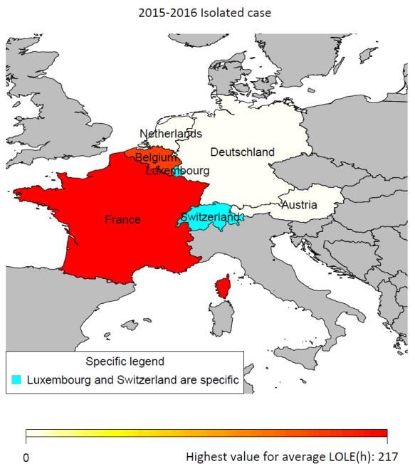
Description           Pentalateral generation adequacy probabilistic assessment
Version               This version of the report is meant for distribution within PLEF SG2 only and not for
                      publication beyond PLEF SG2.
Date                  05. March 2015
Status                    Draft             Final version

Disclaimer:

It must be noted that the conclusions in this report are inseparable to the hypotheses described and can only be
read in this reference framework. The hypotheses were gathered by the TSOs according to their best knowledge
at the moment of the data collection and validated by ministries and regulators. The TSOs emphasise that the
TSOs involved in this study are not responsible in case the hypotheses taken in this report or the estimations
based on these hypotheses are not realised in the future.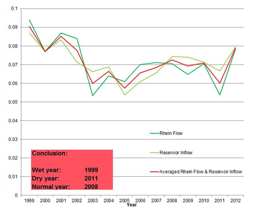
Table of contents
1 Executive summary ........................................................................................................................ 1
2 Approach & Objective .................................................................................................................... 2
3 Methodology ................................................................................................................................. 3
3.1 Advanced tools ......................................................................................................................... 4
3.1.1 Use of multiple models and outputs comparison ..................................................... 5
3.1.2 Assumptions for basic parameters ............................................................................ 6
3.2 Scenario settings ....................................................................................................................... 7
3.3 Data definition .......................................................................................................................... 8
3.3.1 Load........................................................................................................................... 8
3.3.2 Wind, Solar, Other-RES, Other Non-RES ................................................................... 9
3.3.3 Hydro data .............................................................................................................. 10
3.3.4 Thermal units .......................................................................................................... 12
3.3.5 Prices: fuel and CO2 ................................................................................................ 13
3.3.6 Perimeter ................................................................................................................ 13
3.3.7 Import/Export capacity ........................................................................................... 16
3.3.8 Reserves .................................................................................................................. 16
3.4 Analyses conducted ................................................................................................................ 17
3.5 Convergence of the probabilistic assessment ......................................................................... 18
3.6 Adequacy indicators ............................................................................................................... 18
4 Input data .................................................................................................................................... 20
4.1 PLEF region ............................................................................................................................. 20
4.2 Country specifics ..................................................................................................................... 23
4.2.1 Austria ..................................................................................................................... 23
4.2.2 Belgium ................................................................................................................... 24
4.2.3 France ..................................................................................................................... 25
4.2.4 Germany ................................................................................................................. 27
4.2.5 Luxembourg ............................................................................................................ 28
4.2.6 Switzerland.............................................................................................................. 29
4.2.7 The Netherlands ...................................................................................................... 30
4.2.8 Italy, Spain and Great Britain .................................................................................. 32
5 Results of the adequacy assessment ............................................................................................ 36
5.1 Results summary ..................................................................................................................... 36
5.1.1 PLEF Region results reporting ................................................................................. 37
5.1.2 Results reporting for PLEF countries (2015/16 and 2020/21) ................................. 40
5.2 Sensitivity analysis .................................................................................................................. 54
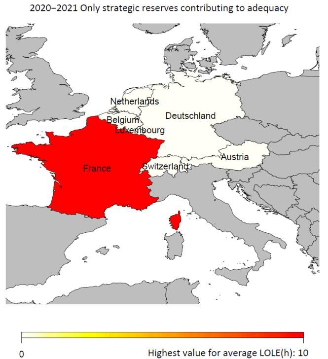
5.2.1 Reserves contribution to adequacy ........................................................................ 54
5.2.2 Results 2012 climate year for 2015/16 and 2020/21 simulations ........................... 57
5.2.3 PLEF region isolated and interconnected ................................................................ 59
5.2.4 Impact of unit decommissioning uncertainty in Belgium for 2015/16 .................... 62
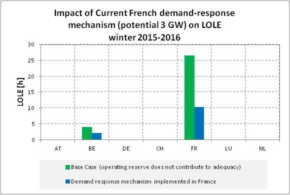
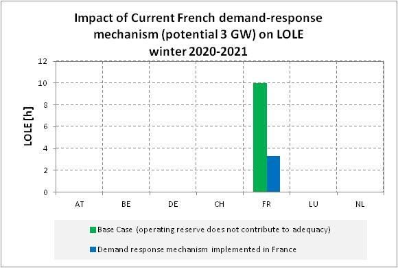
5.2.5 Demand side response 2015/16 and 2020/21 ........................................................ 63
5.3 Conclusions ............................................................................................................................. 65
6 Lessons learnt .............................................................................................................................. 66
7 Next steps .................................................................................................................................... 67
8 Appendix ..................................................................................................................................... 68
8.1 Model descriptions ................................................................................................................. 68
8.1.1 Antares .................................................................................................................... 68
8.1.2 In-house tool Amprion ............................................................................................ 70
9 Glossary ....................................................................................................................................... 72
10 Contact ........................................................................................................................................ 73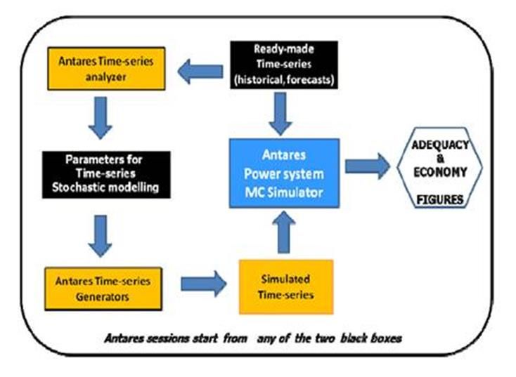
List of figures

Figure 1 Methodology Summary ................................................................................................................................ 3
Figure 2 Use of Multiple Models ................................................................................................................................ 5
Figure 3 Feedback-loops related to the Use of Multiple Models ............................................................................... 6
Figure 4 An Example of Winter Gradient for Switzerland .......................................................................................... 8
Figure 5: An Example of Demand Sensitivity to Several Weather Conditions in France ............................................ 9
Figure 6 Correlation between RoR production and Rhein flow ............................................................................... 10
Figure 7 Correlation between Storage Production and Reservoir Inflow ................................................................ 11
Figure 8 Aggregated Weighted Average of Water Quantity and the Different Hydrological Years ......................... 11
Figure 9 Distribution of Likelihood of Occurrence of the Different Hydrological Years ........................................... 12
Figure 10a Remaining Capacity minus Adequacy Reference Margin 2015 in GW ................................................... 15
Figure 11 Overview of the Modelling Detail of the PLEF and its Surroundings ........................................................ 16
Figure 12 Average Daily Temperature in France ...................................................................................................... 18
Figure 13 Graphical Illustration of the Amount of Monte-Carlo Years Required for Convergence .......................... 18
Figure 14a Generation mix (installed capacities) of PLEF modelled countries [%] 2015-2016 ................................ 20
Figure 15a Installed capacity PLEF countries per fuel type and renewable type [GW] 2020-2021 .......................... 21
Figure 16a Generation mix (installed capacities) of Austria, 2015-2016 ................................................................. 23
Figure 17a Generation mix (installed capacities) of Belgium, 2015-2016 ................................................................ 25
Figure 18a Generation mix (installed capacities) of France, 2015-2016 .................................................................. 26
Figure 19a Generation mix (installed capacities) of Germany, 2015-2016 .............................................................. 27
Figure 20a Generation mix (installed capacities) of Luxemburg, 2015-2016 .......................................................... 28
Figure 21a Generation mix (installed capacities) of Switzerland, 2015-2016 .......................................................... 30
Figure 22a Generation mix (installed capacities) of the Netherlands, 2015-2016 ................................................... 31
Figure 23a Generation mix (installed capacities) of Italy, 2015-2016 ...................................................................... 32
Figure 24a Generation mix (installed capacities) of Spain, 2015-2016 .................................................................... 33
Figure 25a Generation mix (installed capacities) of Great Britain, 2015-2016 ........................................................ 34
Figure 26 Graphical and numerical representation of regional results for year 2015/2016 .................................... 38
Figure 27 Graphical representations (yearly and hourly) of regional remaining capacity for year 2015/2016 ....... 38
Figure 28 Graphical and numerical representation of regional results for year 2020/2021 .................................... 39
Figure 29 Graphical representations (yearly and hourly) of regional remaining capacity for year 2020/2021 ....... 39
Figure 30 Individual country results for year 2015/2016: Austria............................................................................ 40
Figure 31 Individual country results for year 2020/2021: Austria............................................................................ 41
Figure 32 Individual country results for year 2015/2016: Belgium .......................................................................... 42
Figure 33 Individual country results for year 2020/2021: Belgium .......................................................................... 43
Figure 34 Individual country results for year 2015/2016: France ............................................................................ 44
Figure 35 Individual country results for year 2020/2021: France ............................................................................ 45
Figure 36 Individual country results for year 2015/2016: Germany ........................................................................ 46
Figure 37 Individual country results for year 2020/2021: Germany ........................................................................ 47
Figure 38 Individual country results for year 2015/2016: Luxembourg ................................................................... 48
Figure 39 Individual country results for year 2020/2021: Luxembourg ................................................................... 49
Figure 40 Individual country results for year 2015/2016: Switzerland .................................................................... 50
Figure 41 Individual country results for year 2020/2021: Switzerland .................................................................... 51
Figure 42 Individual country results for year 2015/2016: The Netherlands ............................................................ 52
Figure 43 Individual country results for year 2020/2021: The Netherlands ............................................................ 53
Figure 44 Sensitivity results: impact of operational reserves for year 2015/2016................................................... 55
Figure 45 Sensitivity results: impact of operational reserves for year 2020/2021................................................... 55
Figure 46 Sensitivity results: impact of all reserves for year 2015/2016 ................................................................. 56
Figure 47 Sensitivity results: impact of all reserves for year 2020/2021 ................................................................. 56
Figure 48 Sensitivity results: climate year 2012 for year 2015/2016 ....................................................................... 57
Figure 49 Sensitivity results: climate year 2012 for year 2020/2021 ....................................................................... 58
Figure 50 Geographical representation of regional results for year isolated case 2015/2016 ................................ 59
Figure 51 Comparison of results for isolated and interconnected cases for year 2015/2016 ................................. 60
Figure 52 Geographical representation of regional results for year isolated case 2020/2021 ................................ 60
Figure 53 Sensitivity results: effect of decommissioning in BE for year 2015/2016 ................................................ 62
Figure 54 Sensitivity results: effect of DSR in FR for year 2015/2016 ...................................................................... 63
Figure 55 Sensitivity results: effect of DSR in FR for year 2020/2021 ...................................................................... 63
Figure 56 Capacity utilisation on the German French border for year 2015/2016 .................................................. 63
List of tables

Table 1 Definition of the different hydrological years ............................................................................................. 10
Table 2 Probability of the Different Hydrological Years ........................................................................................... 12
Table 3 Raw Input Data for Fuel and CO2 Emission Prices ....................................................................................... 13
Table 4 Derived “RC-ARM” Values for PLEF First and Second Neighbours (2015/16 and 2020) .............................. 14
Table 5 Summary of the Analyses Conducted .......................................................................................................... 17
Table 6 Generation Capacity in the PLEF region ..................................................................................................... 35
Table 7 Overview of results: average LOLE (h) at national and regional level ......................................................... 36
PLEF Adequacy Assessment                                                                          – Final Report –

1     Executive summary

The study mandated by the Pentalateral Forum to the TSOs has been fully and successfully completed. This study
has been a significant step towards a harmonised regional adequacy assessment. It has been performed using a
probabilistic and chronological approach with an hourly resolution for the year 2015/2016 and the year
2020/2021.
The results found in this study are consistent with those found in the corresponding national studies, i.e. poten-
tial adequacy problems are identified for France and Belgium in winter 2015/2016 due to the closure of many
fossil fuel units which are not expected to be upgraded to meet the requirements of the Industrial Emission
                        st
Directive by January 1 2016 or due to mothballing of production units for economic reasons. The adequacy
issues are expected to improve in 2020/2021 due to different measures taken by the affected countries, which
have been in turn integrated into the study through the dataset. Risk exists in France for winter 2020/2021 but
below the national criteria for security of supply. France and Belgium appear as the only countries which require
further investigations through more advanced and specific modelling.
Moreover, the comparison of the results from interconnected and isolated cases reflect how regional exchanges
are vital for security of supply. Yet, a comparison of the adequacy indicators at regional and national level reveals
that most often Belgium and France would experience adequacy risk simultaneously. This result stresses the
added value of studies at regional perimeter as already implemented by Elia and RTE for their own national stud-
ies.
The approach adopted in this study is a tremendous improvement in comparison to the existing deterministic
approaches. Yet, with any simulations, various assumptions must be made for such studies. Some of the most
basic and necessary assumptions include a simplified generation and grid representation (copperplate for each
country except for Luxembourg), system marginal prices solely being marginal costs and perfect insight and fore-
casts in the Day-Ahead markets. Indeed, the methodology employed in this study is similar to the ones already
implemented in Belgium and France, with both probabilistic modelling and regional perimeters, and to the target
one for ENTSO-E as specified in their roadmap for improvement of adequacy assessment in the next few years.
One of the other main achievements of this study is the common regional dataset based on the same scenarios
and assumptions collected and prepared by the PLEF TSOs. For example, it is the first time that a regional-wide
temperature-sensitive load model and harmonised probabilistic hydrological data have been employed. In the
process the TSOs exchanged their technical know-hows of their related systems and adequacy methodologies
and strengthened their collaboration through the regional initiative. Meaningful sensitivity analyses have also
been conducted to evaluate how different important factors can affect the adequacy assessment results. The
extreme cold front in winter 2012 was an important sensitivity which demonstrates how cold weather regional
wide can have severe impact on load and subsequently the ability of the region to match demand and supply.
The sensitivity analyse with different combinations of reserves show how operational and strategic reserves can
have an impact on affected countries. An extra analysis has been conducted for Belgium because two of the
nuclear units have been taken offline unexpectedly during the course of the study.
The potential impact of demand side response (DSR) on adequacy is non-negligible and has been demonstrated
in the sensitivity analyse in which the currently known DSR in France was included in the simulations. However,
cross border exchange of DSR might not always have an impact on the neighbours in need, derived from a con-
clusion coming from the analysis on the usage of interconnection between France and Germany. The analysis
shows that the interconnector would be already completely utilised in times France might have shortages, imply-
ing that any additional available capacity in Germany, e.g. in form of DSR, would not have an impact on the indi-
cators for France.

March 2015                                                                                                  Page 1
PLEF Adequacy Assessment                                                                                      – Final Report –

2      Approach & Objective

Over the past decade, Transmission System Operators (TSOs) significantly improved their cooperation and coor-
dination on security of supply. Within the framework of the Pentalateral Energy Forum1, TSOs cooperate on a
regional basis with governments, regulatory authorities, market parties and power exchanges to improve elec-
tricity markets integration and security of supply. The added value of this regional perspective lies in its ability to
move faster, to reach more specific recommendations and to act as a development centre for new ideas.

The Memorandum of Understanding of the Pentalateral Energy Forum (2007) laid the foundation for a first ade-
quacy forecast for the whole region, by using a bottom-up approach compiling national scenarios. At their meet-
ing on the 7th of June 2013, the Ministers of Energy of the Pentalateral Energy Forum acknowledged the initial
steps on regional adequacy forecasting but also stressed the need to better take into account the current chal-
lenges from the energy transition, with changing generation patterns and market dynamics.

In the Political Declaration of the Pentalateral Energy Forum (2013), the Ministers therefore requested the Penta
TSOs to deliver an enhanced pentalateral adequacy assessment. The analysis should be based on an advanced
new common methodology, including a probabilistic modelling for all hours of the year and enabling a more
consistent assessment of variable renewable energy generation, projected interconnector flows, demand side
management and flexibility in the market.

This Pentalateral Adequacy Assessment offers an essential contribution to the development of a common ap-
proach to security of supply. It provides decision-makers with a more holistic assessment of potential capacity
scarcities in the pentalateral region. And, more importantly, it illustrates the potential support each country can
receive or give resulting from possible economic exchanges arising from the variety of generation mixes in the
region.

In this study an advanced probabilistic adequacy assessment methodology for the PLEF region (AT, BE, CH, DE,
FR, LU, NL) is applied for the first time. Such approach is different from the current methodology applied at the
Pan-European level (ENTSO-E). The latter in comparison is a rather simplistic approach which is based on reserve
margins assessment at only two specific time points in a year, while the PLEF approach provides results on an
hourly basis for the whole year. This study can therefore serve as a pioneer of applying the advanced methodolo-
gy for a wide scale perimeter (regional and pan-European).

The purpose of this report is to describe the methodology and disseminate the results of the adequacy assess-
ment based on this advanced methodology to the Forum, while illustrating the benefits of a common regional
PLEF assessment addressing the requirements of the region.

The layout of the report is given as follows: chapter 1 provides the executive summary of this report. While chap-
ter 2 provides a short description of the approach and objective of the study, the detailed description of the
methodology including the underlying assumptions of the data and parameters is provided in chapter 3. The
description and explanation of the adequacy indicators is also given in this chapter. In chapter 4 the input data
for the PLEF region and its countries are described. The results of the adequacy assessment for the different
scenarios are reported and analysed in chapter 5. The conclusions of the whole study are given at the end of this
this chapter. The lessons learnt in the whole process are summarised in chapter 6 while chapter 7 describes the
possible next steps. In chapter 8, the Appendix, a description of the simulation tools employed in the study can
be found. Glossary is given in chapter 9.

1
  The Pentalateral Energy Forum is the framework for regional cooperation in Central Western Europe towards improved elec-
tricity market integration and security of supply. It was created in 2005 by the Ministers of Energy of Benelux, France and
Germany who aim to give political backing to a process of regional integration of electricity markets. In 2011, Austria joined the
initiative and Switzerland became an observer.

March 2015                                                                                                              Page 2
PLEF Adequacy Assessment                                                                          – Final Report –

3     Methodology

The methodology for this assessment will be characterised by the use of advanced tools. Two different tools will
be used alongside each other. This will enable the analysis of lots of different extreme situations and adequacy
problems will be looked at from different angles. Deterministic as well as probabilistic studies can be covered by
the tools. This topic is described in section 3.1. Another improvement of the methodology lies in the collection of
specific input data for this study. To perform an adequacy study it is important to cover all country specifics. For
the PLEF region this means that temperature sensitivity to load and hydro modelling should be treated with care.
Due to the increasing amount of intermittent energy sources, it is also very important to take this properly into
account. All the input parameters will be elaborated upon in section 3.3.

In order to have a consistent data set, a common scenario is agreed upon. The scenario is based on and built
upon the ENTSO-E scenario A, which is a rather conservative scenario. It is important to detect possible problems
in the region in time, so that necessary actions can be taken. The focus of the study is on two time horizons: the
winter of 2015 and 2020. The scenario settings will be described in section 3.2.

A probabilistic approach: future supply and demand levels are compared by simulating the operations of the
European power system on an hourly basis over a full year. These simulations take into account the main contin-
gencies susceptible of threatening security of supply, including outdoor temperatures (which result in load varia-
tions, principally due to the use of heating in winter), unscheduled outages of nuclear and fossil-fired generation
units, amount of water resources, and wind and photovoltaic power production.

A set of time series, loads on the demand side and available capacity of units generating supply reflecting various
possible outcomes are created for each of the phenomena considered. These series are then combined in suffi-
cient number to give statistically representative results in shortages (risk of demand not being met due to a lack
of generation) and annual energy balances (output of different units and exchanges with neighbouring systems).

Adequacy criteria are often defined on a national level. In this study adequacy indicators are additionally calcu-
lated on a regional level. These indicators will be described in section 3.6.

Although the proposed methodology has some significant improvements over the current ENTSO-E methodology,
the methodology is still open to further improvements, for example flow based modelling or the extension of the
climate database to cover more representative samples of the climatic variations. Some further improvements
will be listed in the next steps. However, the envisaged work with improved parameters for the PLEF region will
be very valuable as a test case for future use on an ENTSO-E scale. A summary of the methodology is shown in
the following figure.

                                         Figure 1 Methodology Summary

March 2015                                                                                                 Page 3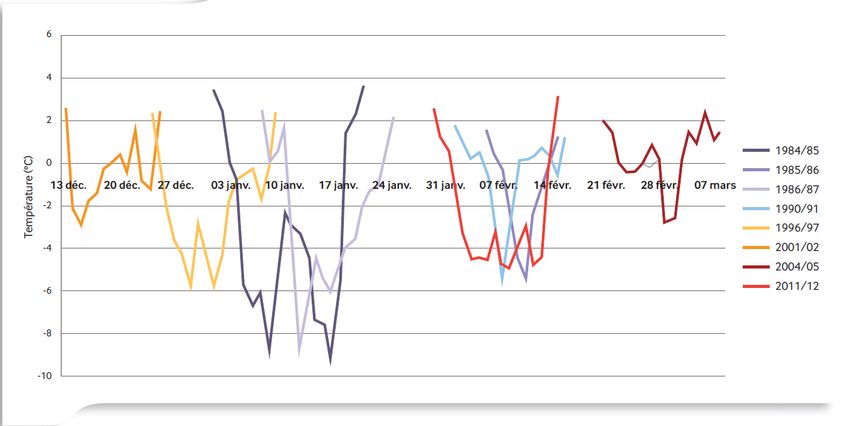
PLEF Adequacy Assessment                                                                             – Final Report –

3.1     Advanced tools

In this section a general description on the tools employed for the PLEF adequacy analyses is given. This includes
the main features one can expect from these tools. For the specific features which come with individual tools
employed in the study please refer to the Appendix, where one could find more detailed description for Antares
and the Amprion’s inhouse tool.

In general the tools employed are built upon a market simulation engine. Such market simulation engine is not
meant for modelling or simulating the behaviour of market players, e.g. gaming, explicit capacity withdrawal
from markets, etc., but rather meant for simulating marginal costs (not prices) of the whole system and the dif-
ferent market nodes. Therefore the main assumption is that the markets function perfectly.

The tools calculate the marginal costs as part of the outcome of a system-wide costs minimization problem. Such
mathematical problem, also known as “Optimal Unit Commitment and Economic Dispatch” is often formulated as
a large-scale Mixed-Integer Linear-Programming (MILP) problem. In other words, the program attempts to find
the least-cost solution in which no operational constraints (e.g. ramping, minimum up/down time, transfer capac-
ity limits, etc.) are violated. In order to avoid infeasible solutions very often the constraints are modelled as “soft”
constraints, which means that they could be violated, but at the expense of a high penalty, i.e. high costs. Most
mathematical solvers nowadays are capable of solving large-scale LP problems with little computation time.
However, with the presence of integer variables it is still common in commercial tools to solve the overall prob-
lem by applying a combination of heuristics and LP.

In the regional study for PLEF, the size of the problem, i.e. the number of variables and constraints could be huge,
i.e. thousands of each of them. The size increases with the optimization time horizon and the resolution. For the
PLEF study the horizon is a week and the resolution is hourly, i.e. given the constraints and boundary conditions
the total system costs are minimized for each week on an hourly basis. The weekly optimization horizon means
that the optimal values for each hour of the whole year are calculated, with the optimization problem broken up
on a weekly basis, in order to reduce the computation time. A weekly optimization horizon is also a common
practice for market simulations at many TSOs for network planning. The latter means that the results such as
generation output of the thermal and hydro plants, marginal costs, etc. are given per hour. This setting of the
parameters is also the common practice for the market simulations which are conducted for ENTSO-E TYNDP.

These tools also have the functionality to include the network constraints to a different degree. Nowadays the
status quo approach pan-European or regional market studies is based on NTC/ATC-Market Coupling (NTC/ATC
MC). This means that the network constraints between the market nodes are modelled as limits only on the
commercial exchanges at the border. This approach is used in this study.

The EU target model is based on Flow-Based Market Coupling (FBMC). In this model the network constraints are
modelled as real physical limits on selected “critical branches”. Most TSO tools nowadays can do FBMC, even
though they have not been thoroughly tested for large-scale applications. There are also tools which can model
the physical network including all the technical constraints such as contingencies, thermal and voltage con-
straints, therefore supporting what is commonly known as OPF (Optimal Power Flow). Such feature is not yet
common in Europe since there is no agreement or plans for a regional scale application of nodal pricing.

Most of the market simulation tools can be used for adequacy analysis purposes. For probabilistic modelling
Monte-Carlo simulation is required. This involves a large number of simulations with random draws (combina-
tions) on the stochastic variables (e.g. climate data, load, hydrological conditions, forced outages etc.) in order to
work out a probability distribution curve of the required outputs (e.g. ENS, LOLE). To facilitate this, the tools
would have features which enable easy handling of these additional inputs and outputs, e.g. multiple time series
of load, solar, wind etc. and the corresponding outputs, in a probability distribution curve, etc. In order to reduce
the time required for this big number of simulations, some tools also have a “quick-run” feature which reduces
convergence time significantly for each run through the simplification of the optimization problem (e.g. removing
integer variables, i.e. the on/off decisions, the ramping constraints, etc.).

It is important to mention that the use of multiple tools with the same dataset as inputs, though more time-
consuming, improves the quality of the results since debugging of the inputs and models as well as the bench-
marking of the results can be facilitated.

March 2015                                                                                                    Page 4
PLEF Adequacy Assessment                                                                        – Final Report –

3.1.1    Use of multiple models and outputs comparison

For this study two different models (Antares and the Amprion’s inhouse tool) were used in parallel. The aim of
the use of different models and the comparison of the model outputs is to create consolidated, representative
and reliable results. The process is shown in Figure 2. The comparison of the results was done for a “reference
year” (2015-2016, weather data 2007-2008, normal hydro conditions) and it was done in four steps:
    -    Preparation of aggregated output data of the models
    -    Visualization of the output data in form of comparison charts
    -    Discussions and analyses within the PLEF TSO group
    -    Specification of actions regarding model or data improvement
The comparison was done three times during the whole course of the project.

                                        Figure 2 Use of Multiple Models

Although the use of multiple models and the output comparison is a lengthy and time consuming procedure,
some major advantages are connected to it e.g.:

    -    Input data quality: Owing to the fact that multiple models are used the input data are checked multiple
         times independently. This way, errors in the input data will be detected more likely and can be correct-
         ed. See also feedback loop no. 3 in Figure 3. This leads to a consistent set of input data and at the same
         time input data of high quality.

    -    Synchronization of input data: Some of the input data are also part of the aggregated output data of
         the models (e.g. PV feed-in, load per country). This way possible input data differences (between the
         different models) can be detected and corrected. The synchronization of the input data is the basis for
         the comparison of the actual results and also helps to gain a common understanding of the input data.
         See also feedback loop no. 2 in Figure 3.

    -    Comparison of results: The identification of differences in the results of the models, enables a discus-
         sion about e.g. how the models work and how the modelling (e.g. of hydro power plants, biofuel units)
         is done. Furthermore it also enables a discussion about the influence of model parameters that are not
         part of the aggregated output data (e.g. fuel and CO2 prices). This leads to an adaptation of the model-
         ling (see feedback loop no. 1 in Figure 3) and subsequently to a better understanding of the influence
         some of the parameters (e.g. outages) have on the system.

March 2015                                                                                                Page 5
PLEF Adequacy Assessment – Final Report –
Figure 3 Feedback-loops related to the Use of Multiple Models
If the described process with its feedback-loops is followed thoroughly a better understanding of the results and
also higher quality results can be obtained. In our case the results of the models converged although some differ-
ences remained. Overall it was possible to increase the confidence in the results.
3.1.2 Assumptions for basic parameters
In this section the assumptions for some of the generic parameters applicable to all tools are briefly described.
The technical details for each of the tools might differ and are described in the user manuals.
Hydro modelling, weekly profiles
Since the optimization horizon in the simulations is on a weekly basis, the information regarding reservoir inflow,
river flow as well as reservoir level is predefined and given as inputs which are treated as constraints in the opti-
mization. In the PLEF simulations the tools are fed with weekly or monthly profiles to define the boundary condi-
tions for the optimization.
Modelling a hydro production system, especially one including storage and pump storage power plants is chal-
lenging due to its complexity and the presence of many stochastic variables, e.g. cascades of reservoir basins and
unclearly defined marginal costs. Therefore some simplifications have to be made. As the optimization horizon of
the simulations is on a weekly basis, the weekly starting and ending levels of the reservoir of annual storages are
treated as constraints in the optimization. These weekly values are either found from interpolation, e.g. for res-
ervoir level, or from equally dividing the monthly values, e.g. for flow quantity. The marginal costs for hydro
production are by default zero. This means that hydro units will be committed before thermal units. But within
the week the simulation tries to reach a minimum system cost using all dispatchable units such as pump storages,
storages and thermal units. In this way hydro dispatch is dependent on market price signals in the whole week,
i.e. opportunistic costs. For reservoir power plants min/max of pumping and turbining capacities are additional
optimization constraints. Natural reservoir inflow per week is also predefined and given in different profiles (time
series) according to different hydrological years (wet, normal, dry). For run-of-river the amount of energy which
has to be produced within the week is predefined.
Therefore, in the PLEF simulations the tools some of the important parameters on a hydro system are based on
historical hydrological values. It should be noted that the weekly reservoir levels and constraints can in theory be
optimized and calculated for each scenario with the aid of a long-term optimization tool. This step has not been
performed for the PLEF studies.
Outages & maintenance draws
Every thermal unit is given a rate of unavailability that is based on the type and fuel of the unit. Those values are
the reference values used in ENTSO-E studies and come from historically observed forced unavailability of units.
The simulation tool will choose which unit will be unavailable based on these rates. Every draw of outages will be
different but the average over a period of time is the same. This method allows the simulation of different com-
binations of outages and extreme events.
March 2015 Page 6PLEF Adequacy Assessment – Final Report –
Interconnector availability
The maximum commercial transfer capacity between different countries is defined by the value of the NTC. In
the annual PLEF simulations two NTC values are used: one for winter and one for summer. In practice however
the NTC values given to the market changes every hour because of different factors such as outages, mainte-
nance as well as temperature affecting the thermal transfer capacity of the transmission lines. The winter and
summer values used for the simulations represent the average of the hourly fluctuating values.
3.2 Scenario settings
Corner stones of the generation adequacy assessment
In order to give a clear picture of the expectations on this adequacy study it should be stated that this study will
model the power system using predefined situations described in scenarios. Also the commissioning and de-
commissioning of generation capacities are given exogenously with the scenario definition. The adequacy as-
sessment study will model how this given production will meet the forecasted demand but should not lead to
statements on whether or not the market works properly or investments will be made in the near future. This
stems especially from the fact that a central optimized dispatch is simulated – not a bottom up market – and the
available generation capacity is given exogenously. Targeted market modelling exercises are more suitable to
derive information such as optimal installed capacity of generation facilities.
PLEF time horizons
The following years have been identified to give a complete overview of the adequacy situation in the short-term
and mid-term time horizon in the countries of the Pentalateral Energy Forum (what is referred to as “PLEF” in the
report).
01.10.2015 – 30.09.2016 – short-term analysis
01.10.2020 – 30.09.2021 - mid-term analysis
Scenario for short-term analysis: PLEF Scenario 2015
For the short-term adequacy assessment (10/2015 – 09/2016;) the scenario “PLEF Scenario 2015” has been de-
fined mostly based on the conservative ENTSO--E Scenario A given in the Scenario Outlook & Adequacy Forecast
2013-2030 (SO&AF). The PLEF scenario 2015 uses generation capacities which are available by 1st of October of
2015.
The PLEF scenario (or conservative scenario) is a bottom up scenario taking into account only confirmed addi-
tional investments in generation to maintain the current level of supply. Only the commissioning of new power
plants which are considered as confirmed according to the information available to the TSOs are taken into ac-
count. The same approach is taken for the decommissioning of existing power plants. Corrections with respect to
closure and temporary shutdown of generation assets will be taken into account if possible.
Contrary to the ENTSO-E Scenario A in the PLEF scenario renewable generation is taken into account on the basis
of the “best estimation” of the TSOs as in the most cases the commissioning of renewables are not confirmed in
an early stage.
Also Load forecasts are the best national estimates available to the TSOs under normal climatic conditions. A
more detailed description on load modelling is given in section 3.1.1.
For the short-term scenario Fuel and CO2 prices are based on the “Current Policies Scenario” used in the IEA
report World Energy Outlook 2013. More description is given in section 3.3.5.
Scenario for mid-term analysis: PLEF Scenario 2020
For the mid-term adequacy assessment (10/2020 – 09/2021) the scenario “PLEF Scenario 2020” has been de-
fined. This scenario is based on the same approach as the "PLEF Scenario 2015".
Harmonization of data for scenarios
In order to improve the quality of the assessment, all scenarios make use of:
a common approach of RES (solar and wind) availability based on historical climate data,
correlated and synchronized hydro data for specific hydrological conditions (“normal”, “dry” and “wet”
years) for Switzerland, Austria and France and Germany,
temperature sensitivity of load with a common approach by using time series of temperature from the
ENTSO-E climate database (correlated to the solar and wind time series)
March 2015 Page 7PLEF Adequacy Assessment – Final Report –
3.3 Data definition
In addition to an improved methodology, TSOs will also use improved data. Correlated weather data on the one
hand, allowing the production of time series of wind and solar generation, and improved hydro data on the other
hand, making it possible to show important correlations with climatic conditions. The temperature sensitivity is
one of the big drivers for this study. More details are described in the following sub-sections.
3.3.1 Load
Load is a very important input parameter in a generation adequacy assessment. A lot of effort is put in calculating
correlated input data between the different countries.
As a starting point the TSOs delivered a normalized load profile (no temperature sensitivity) for the coming years
according to their best estimate of growth rate using the calendar of the year 2007.
As a second step the sensitivity to temperature is added to the load profiles according to common and correlated
data, since weather conditions can significantly affect electricity demand in some countries of the PLEF region. A
widespread use of electric heating is the primary factor explaining the surge in demand observed during cold
spells in winter and leads to high demand fluctuations from one year to the next.
A “temperature-sensitivity-model” was developed and implemented to address this issue. It offers two features:
1. Define the current winter temperature sensitivity for each country
2. Define load time series for each country based on temperature data and the defined temperature sensitivity
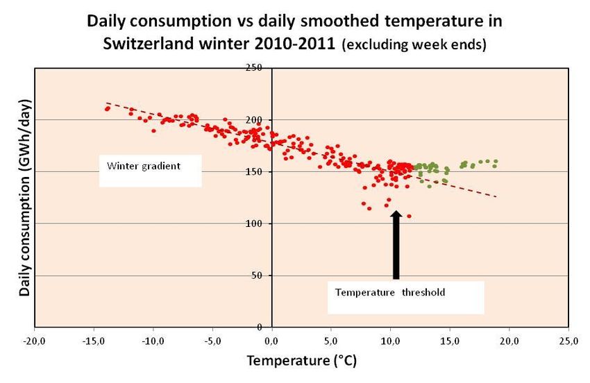
The model determines the current thermo-sensitivity based on historical demand data and corresponding tem-
perature data from the Pan-European Climate Database (PECD). The model is structured around three comple-
mentary concepts: gradient, threshold temperature and smoothed outdoor temperature during the winter
months (see also Figure 4):
Gradient (MW/°C) represents the increase in power demand corresponding to a given drop in temperature
Threshold temperature corresponds to the temperature below which demand becomes sensitive to weather
condition
Smoothing of outdoor temperatures takes into account various phenomena, such as thermal inertia of
buildings, human factors and the influence of cloudiness
Figure 4 An Example of Winter Gradient for Switzerland
All the countries whose sensitivity to temperature is significant used the proposed model to define the winter
gradient.
Based on the demand time series under normal conditions, temperature data from the PECD (Pan European
Climate Database) and estimated winter gradient, load time series under several climatic conditions are built for
several years. As a first approximation we consider that our climate data base covers a representative sample of
the climatic variations. As a consequence normal temperature corresponds to the average temperature of the
PECD. As an example the graph below shows the demand sensitivity to several weather conditions for France.
March 2015 Page 8PLEF Adequacy Assessment – Final Report –
Load for France for one year (starting 1st Oct.)
Red: Load under normal conditions
Blue: Load for the years 2001 – 2011
Figure 5: An Example of Demand Sensitivity to Several Weather Conditions in France
A topic closely related to demand data is interruptible demand capacity or demand response (DSR). TSOs con-
firm that this issue is very relevant for generation adequacy assessment, but also a very difficult one because of
the different contracts that are behind this capacity for different countries. Therefore, simplified modelling of
DSR is taken into account as an extra sensitivity (see chapter 5.2.5)
3.3.2 Wind, Solar, Other-RES, Other Non-RES
The modelling of wind, solar and other renewable capacity and energy in-feed in the adequacy assessment is
challenging mainly due to two reasons: availability of these energy sources in case of scarcity and the uncertainty
of new installed capacity in operation according to the national remuneration policies in place or changing in the
coming years. The RES installed capacity is based on TSO best estimates. Improvements regarding the availability
of these RES units have been used.
Wind/solar
Historical load data coupled with the usage of the PECD (Pan European Climate Database) containing 12 years of
hourly correlated wind, solar and temperature data, enables the correlation of demand, wind and solar in-feed.
Together with TSOs best estimates on the increase of wind and solar capacities in the coming years the hourly
availability or these renewable units can be forecasted assuming that these units will be used in a similar way as
in the past. During this study the available PECD data were updated with weather data of the year 2012. The
beginning of 2012 was distinguished by a cold spell. To improve the results of this assessment the extended PECD
data (wind, solar and temperature) were used for sensitivity calculations.
Other RES / Other non-RES
Other RES (other renewables)
For each market node and scenario the total installed capacities (GW) and hourly time series (MW) of non-
despatchable generation out of all renewables which have not been depicted elsewhere are provided. This cate-
gory is simulated as an inflexible source and is not price-driven. Below a non-exhaustive list of Other RES genera-
tion:
• Tidal generation
• Wave generation
• Geothermal generation
• Biomass
• Waste (renewable)
Other non-RES (other non-renewables)
For each market node and scenario the total installed capacities (GW) and hourly time series (MW) of non-
despatchable generation out of all non-renewables which have not been depicted elsewhere are provided. This
category is simulated as an inflexible source and is not price-driven. Below examples of Other non-RES genera-
tion:
• Combined Heat and Power (CHP)
• Waste (non-renewable)
March 2015 Page 9PLEF Adequacy Assessment – Final Report –
3.3.3 Hydro data
A good probabilistic representation of the hydro generation system is required for the PLEF region because there
is significant amount of hydro installed capacity in three (Austria, France and Switzerland) of the countries in the
region. In the whole region hydro also has a significant role since the total installed hydro capacity amounts to
16% in 2015 (14% in 2020) of the total installed capacity, which ranks the second highest, directly after gas, which
amounts to 21% in 2015 (20% in 2020, followed by 17% of onshore wind). Historical data has shown that the total
annual hydro production can vary up to more than 20% between a dry and a wet year. In particular, in the Alpine
region where seasonal pump-storages are dominant, the hydro electricity production in winter could significantly
reduce in a dry year. This could therefore result in a critical condition when the winter also happens to be cold.
The goal of this exercise is therefore to define suitable hydro profiles which can be used as a common approach
for all PLEF countries taking into account the availability of data. Because of the geographical proximity of these
three countries, it is expected that their hydrological conditions should be closely correlated, i.e. when there is a
dry year in Switzerland, it should also be dry in Austria and France, and vice versa. By applying statistical analyses
three distinctive hydro profiles are derived: “dry”, “wet” and “normal”. To facilitate the probabilistic methodolo-
gy, each of these profiles has to be associated to its corresponding probability, which represents the likeli-
hood/frequency of its occurrence. Each of these profiles contains the weekly values for RoR (Run-of-River), reser-
voir production (storage, pumped storage, and swell power plants) and natural inflow for reservoir.
The definition of the different hydrological years is as follows:
Type of hydrological year Definition
Dry Relatively small amount of aggregated electricity production from all the run-of-
river and reservoir plants
Wet Relatively big amount of aggregated electricity production from all the run-of-
river and reservoir plants, without flooding being caused
Normal Expected amount of aggregated electricity production from all the run-of-river
and reservoir plants
Table 1 Definition of the different hydrological years
To derive these three special hydrological conditions, monthly historical data of the past 14 years (1999-2012) for
the Swiss hydro electricity production from reservoirs, RoR, reservoir levels and pumped consumption were
analysed.
In order to eliminate the influence of the different installed capacities in different years, water quantity, instead
of production, was used (e.g. if installed capacity is increased over time and we would not be able to distinguish if
an increase in production came from the additional installed capacity or from a “wet” year). In order to validate if
this approach – using water quantity instead of electrical production to define the hydrological years - is applica-
ble, the correlation between electricity production and water quantity for RoR and also reservoir power plants
was evaluated. A strong correlation can be found (as shown in the next two diagrams) which leads to the as-
sumption that this approach is feasible.
Figure 6 Correlation between RoR production and Rhein flow
March 2015 Page 10PLEF Adequacy Assessment – Final Report –
Figure 7 Correlation between Storage Production and Reservoir Inflow
In order to use the combined information of river flow rate together with reservoir natural inflow for the deter-
mination of the relevant hydrological years, the weighted average of river flow (Rhein) and reservoir inflow was
calculated and the resulting outcome is shown in the next diagram.
Figure 8 Aggregated Weighted Average of Water Quantity and the Different Hydrological Years
Based on this 1999 was chosen for the wet year, 2011 for the dry year and 2008 for the normal year.
In order to derive a more statistically sound set of probabilities which corresponds to the derived hydrological
years, more historical years needed to be analysed. For this purpose 81 years of RoR river flow was employed. At
the time of the study it was not possible to acquire the same data for water inflow, but instead the RoR data
were representative enough because of the high correlation between the two, as indicated previously. The distri-
bution of the RoR data is plotted in the following diagram.
March 2015 Page 11PLEF Adequacy Assessment – Final Report –
Figure 9 Distribution of Likelihood of Occurrence of the Different Hydrological Years
With this information the likelihood of occurrence of the derived hydrological years was extracted, by comparing
and ranking the amount of hydro quantity of these years among those from the dataset. The representative dry
and wet years were selected based on the probability of about 10% at both sides of the spectrum. The resulting
probabilities are listed in the following table.
Determined Year Probability of occurrence
“Dry” year 2011 10%
“Wet” year 1999 10%
“Normal” Year 2008 80%
Table 2 Probability of the Different Hydrological Years
These values and the hydro data profiles for the different Swiss hydrological years were used in order to derive
the corresponding required input data for the PLEF countries (especially for Austria and France). The probability
of occurrence helped to ensure that the event of having a certain set of conditions (e.g. a dry year) will happen
simultaneously for all the PLEF countries during the Monte-Carlo simulations.
3.3.4 Thermal units
Thermal generation categories and main characteristics
In order to ensure coherency of the market behaviour of thermal units in Europe, and to avoid deviations in the
simulation runs carried out in this study, 22 different categories for thermal power plants were used. These cate-
gories – defined in the guidelines for the Pan European Market Modelling Data Base (PEMMDB) – use standard
values for the main technical and economic characteristics. These thermal categories are dependent on:
fuel (e.g. gas, hard coal, lignite…)
type (e.g. OCGT, CCGT…)
and age (e.g. old 1, old 2, new…), which corresponds to a certain range of efficiency of the power plant.
The despatchable CHPs were assigned to the common used fuel, bearing in mind the consequence on the merit-
order. The fully non-despatchable CHP units were included in the category 'Other RES' (if renewable) or 'Other
2
non RES' (if not-renewable) data set.
2
The CHP operation is an optimisation on its own and it would be difficult to include it in our simulations. Therefore it is mod-
elled with hourly profiles (“Other RES” or “Other non RES”) whenever possible.
March 2015 Page 12PLEF Adequacy Assessment – Final Report –
Considerations
This generation adequacy assessment is carried out on a conservative basis and only takes into account certain
shutdowns or certain commissioning of thermal generation units. With respect to mothballing units:
3
mothballed units will not be considered available to the system and;
only official data will be taken into account .
3.3.5 Prices: fuel and CO2
Fuel and emission prices form part of the basic input dataset required for market simulations. The SO&AF Scenar-
io A dataset defines the installed generation capacity, but unlike the ENTSO-E 2030 visions, it does not include or
give indication on fuel and emission prices. It is therefore necessary to use another known reliable source. For
this the IEA WEO (World Energy Outlook) 2013 edition was chosen, which is also a typical choice for ENTSO-E
TYNDP scenarios.
In the IEA WEO there have been so far seven basic scenarios (with Current Policies, New Policies and 450 ppm
being the most frequently quoted ones). For the PLEF studies the Current Policies Scenario was chosen, which is
defined as follows:
“Current Policies Scenario: A scenario in the World Energy Outlook 2010 (but still being referred to and updated in
later editions) that assumes no changes in policies from the mid-point of the year of publication (previously called
the Reference Scenario)”
The scenarios define the political and economic settings which result in a specific set of fuel as well as emission
prices. In the 2013 edition, however, no data were published for year 2015/2016. Because of that, the values
given in WEO for 2012 and for 2020 were used to interpolate the values for year 2015. The results are shown in
the following table:
Table 3 Raw Input Data for Fuel and CO2 Emission Prices
The values for our simulations are highlighted in red and it is observed that the fuel prices do not vary significant-
ly between the scenarios, except for CO2 prices. The reason for the high value in the 450 ppm Scenario is because
of the limitation on the concentration of greenhouse gases in the atmosphere to about 450 parts per million of
CO2, so that global increase of temperature would be limited to 2 degree Celsius. With the recent development
of CO2 prices this would be an extreme case and therefore is not applicable for the PLEF studies.
When converted to marginal costs, this set of values would result in a typical merit-order (without start-up costs)
which we observe nowadays, i.e. starting from the technology with the lowest cost:
Nuclear < Lignite < Hard coal < Gas < Oil
This is only an indicative merit-order curve, as in the simulation tools the economic dispatch is also determined
by other parameters such as start-up costs, ramping constraints, etc.
3.3.6 Perimeter
The perimeter of the study is not limited to the PLEF region. The so called “ROW“ (Rest Of the World) refers to
the countries which are not in the PLEF region, but are required in the model in order to have a good representa-
tion of the interconnected system between the PLEF countries and the neighbours. Given that data collection is a
very lengthy process and because of our limitation in available resources, we have adopted a pragmatic approach
for the ROW modelling which is described in this section.
All of our first neighbours (i.e. those with a direct electrical connection with the PLEF countries) are modelled, but
in a different degree of detail. For the smaller or less influential countries (see Figure 11: Small 1st neighbours)
we took the ENTSO-E SO&AF (Scenario Outlook and Adequacy Forecast) data and approach. In the SO&AF ap-
3
The TSO do not necessary have information about how long it takes for a mothballed power plant to get back online again. As
the re-activation time might be different for each of the mothballed units TSOs decided to consider these units in the following
way: If a mothballed unit is contracted by a TSO (and can therefore be activated in due time) it is taken into account, if a moth-
balled unit is not contracted by a TSO it will be taken out of the dataset.
March 2015 Page 13You can also read