Trade-Induced Urbanization and the Making of Modern Agriculture
←
→
Page content transcription
If your browser does not render page correctly, please read the page content below
Trade-Induced Urbanization and the Making of Modern Agriculture

                               Yuan Tian, Junjie Xia, and Rudai Yang⇤

                                                June 21, 2021

                                                   Abstract

          Manufacturing growth can benefit the agricultural sector if the outflow of labor from agri-
      culture improves land allocation efficiency and facilitates capital adoption. Using destination
      prefectures’ trade shocks in the manufacturing sector driven by China’s accession to the World
      Trade Organization (WTO) and the origin village’s initial internal migration network, we con-
      struct the exposure to manufacturing trade shocks for a panel of 295 villages from 2001 to 2010.
      We find that villages with larger increases in trade exposure had larger increases in the share of
      non-agricultural laborers, more fluid local land markets, and faster modernization of production
      through the adoption of agricultural machinery. Village-level agricultural productivity improved
      through the allocation of land towards more productive farmers within a village. During the era
      we study, transaction costs declined in the agricultural land market. We use a quantitative model
      to show that the growth in non-agricultural productivity had a larger impact on urbanization
      and agricultural modernization than reductions in transaction costs.
          JEL codes: F16, J24, O14, O4, Q12, Q15.
          Keywords: Land Misallocation, Capital Adoption, Urbanization, Trade Liberalization, Agri-
      culture Modernization

  ⇤
    Tian: University of Nottingham, School of Economics (email: yuan.tian1@nottingham.ac.uk); Xia: Peking Uni-
versity, Institute of New Structural Economics (email: junjiexia@nsd.pku.edu.cn); Yang: Peking University, School
of Economics (email: rdyang@pku.edu.cn). We are grateful to Pablo Fajgelbaum, Brian Kovak, and Adriana Lleras-
Muney for support and guidance. We received valuable feedback from Daniel Berkowitz, Lee Branstetter, Chaoran
Chen, Yi Chen, Karen Clay, Matthew Delventhal, Jingting Fan, Martin Gaynor, Akshaya Jha, Rebecca Lessem,
Bingjing Li, Daniel Nagin, Michael Poyker, Yogita Shamdasani, Allison Shertzer, Lowell Taylor, Xiaodong Zhu, and
participants at various conferences and seminars. All errors are our own.

                                                       1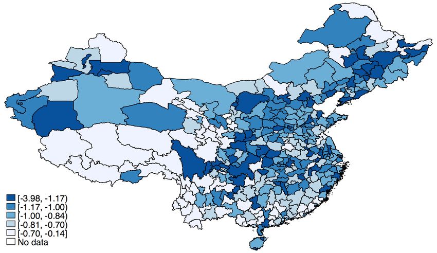
1        Introduction
        No country has achieved a high level of income without a sharp reduction in agricultural em-
ployment and a concomitant modernization of agricultural production.1 The economic literature
on structural transformation hypothesizes two broad explanations on the drivers of this process: i)
technological innovation in the agricultural sector, and ii) increased attractiveness of urban areas
and the manufacturing sector.2 Despite rich theoretical discussions of these two channels, empirical
studies of structural transformation are scarce and focus mostly on the first channel.3
        We fill this gap in the literature by providing empirical evidence on how structural transformation
is initiated by manufacturing growth and reinforced by the development process in agriculture along
a range of dimensions. Using a unique dataset on agricultural households in China, we study how the
manufacturing growth induced by international trade liberalization affected agricultural production
in the context of China’s WTO accession. The pull forces driving migration out of rural areas came
from the reduction in tariffs faced by manufacturing exporters, which resulted in an increase in labor
demand in urban areas. We measure a migrant destination prefecture’s exposure to manufacturing
trade as a weighted average of industry-level tariffs faced by Chinese exporters in their destination
markets, with local industry-level employment as weights. Then, we connect an origin village with
its migrant destination prefectures using the initial prefecture-to-prefecture migration network. A
village was more exposed to manufacturing trade if its destination prefectures on average faced larger
declines in tariffs in export markets.
        We show that increased labor demand in the urban manufacturing sector led origin villages to
shift employment from agriculture to non-agriculture. Rural land markets became thicker, and rental
activity increased. Land allocation efficiency also improved; initially more productive households
operated larger farms, especially in villages that experienced larger destination trade shocks. We
also find that the villages facing larger trade shocks had faster modernization of production through
the adoption of agricultural machinery and increased village-level agricultural productivity.
        As in many other developing countries, rural land markets in China are incomplete, with high
transaction costs of land leasing between farmers.4 The initial land distribution was mostly propor-
tional to household size, no matter how productive an individual or a household was in crop farming.
Yet, before 2000 less than 4% of rural households rented out their land, suggesting that the land
allocation efficiency was low. This situation improved with the substantial growth in manufacturing
trade and fast urbanization after 2000. The share of rural labor working in the non-agricultural
sector increased from 16% in 2000 to 25% in 2010, and the share of households with land rental
    1
     See Lewis [1954]; Schultz et al. [1964]; Taylor and Martin [2001]; Lucas [2004]; and Akram et al. [2017], among
others.
   2
     See Baumol [1967]; Murphy et al. [1989]; Kongsamut et al. [2001]; Gollin et al. [2002]; Ngai and Pissarides [2007];
and Yang and Zhu [2013], among others. Other explanations include the decline in the relative cost of obtaining
non-agricultural skills, as shown in Caselli and Coleman [2001].
   3
     Empirical studies on the channel of technological innovations in the agricultural sector include Foster and Rosen-
zweig [2004, 2007]; Nunn and Qian [2011]; Michaels et al. [2012]; Hornbeck and Keskin [2015]; and Bustos et al.
[2016].
   4
     See Adamopoulos and Restuccia [2014]; de Janvry et al. [2015]; Adamopoulos et al. [2017]; Chen [2017]; and
Restuccia and Santaeulalia-Llopis [2017].

                                                           2
income increased to 13%.
       Our main data set is a nationally representative sample of rural households and villages from the
National Fixed Point (NFP) Survey, with information on agricultural production and rural household
living arrangements. The survey collects information on a panel of around 20,000 Chinese rural
households in 300 villages. We use the 2001–2010 data for the main analysis and the 1995–2001
data to rule out confounding pre-trends.5 We observe household-level occupation choices, land-
in-operation, the amount of land rented from other households, and land transactions during the
year. Using detailed information on output values, labor, capital, land, and intermediate inputs, we
calculate household-level and village-level total factor productivity (TFP) in crop farming.6
       We use cross-sectional variation in the reduction of manufacturing tariffs to generate shocks to
pull-factors for out-migration. Identifying the causal effect of out-migration on agricultural produc-
tion is generally difficult. First, increases in agricultural productivity can lead to more out-migration
if the technological change is labor-saving (Bustos et al. 2016). Second, expansion of rural trans-
portation networks can incentivize out-migration and improve agricultural productivity through
improved input quality. Third, economy-wide productivity shocks can generate correlated produc-
tivity growth in the manufacturing sector and the agricultural sector, and labor can flow out of
agriculture if the manufacturing productivity growth dominates. We overcome these identification
challenges by using the strong forces incentivizing internal migration generated by China’s WTO
accession in 2001 (Facchini et al. 2019; Tian 2020; Zi 2020). We employ a shift-share measure to con-
struct a village’s exposure to destination prefectures’ trade shocks. Following the standard method
in the literature on the local labor market effect of trade liberalization (Topalova 2010; Kovak 2013;
McCaig and Pavcnik 2018; Bombardini and Li 2020; and Tian 2020), a destination prefecture’s expo-
sure to manufacturing trade is measured as a weighted average of industry-level output tariffs faced
by exporters, with each industry’s employment share as weights. A reduction in the average tariff
faced by a prefecture acted as a positive demand shock for the goods produced in the prefecture,
and it resulted in an increase in labor demand in the manufacturing sector.7 An origin village’s
exposure to manufacturing growth is measured as the interaction of its initial migration network
and the destination prefectures’ trade exposures. The prefecture-to-prefecture migration network is
constructed using a sample of one million individuals from the 2000 population census, where an
individual’s residence prefecture in 1995 and current residence prefecture are observed.
       These output tariffs were imposed by importing countries on Chinese exports, and the industry-
level post-WTO tariff reductions were uncorrelated with pre-WTO tariff changes and export growth.
   5
     This is the best available dataset on agriculture production and rural households in China. Adamopoulos et al.
[2017], Kinnan et al. [2018], and Chari et al. [2020], among others, have used different segments of the dataset. To our
knowledge, we are the first to use the full sample of households for a time period that spans before and after China’s
international trade liberalization.
   6
     Our main productivity measure is a Solow residual estimated using a Cobb-Douglas production function. An
alternative measure of agriculture productivity can focus on the labor productivity (Lagakos and Waugh 2013). Our
results on productivity is robust to using the labor productivity.
   7
     Tian [2020] provides evidence on how the output tariff reductions were associated with increased exports at the
industry level in Figure 6, and how the average tariff reductions at the prefecture level led to increased wages in Table
A18.

                                                           3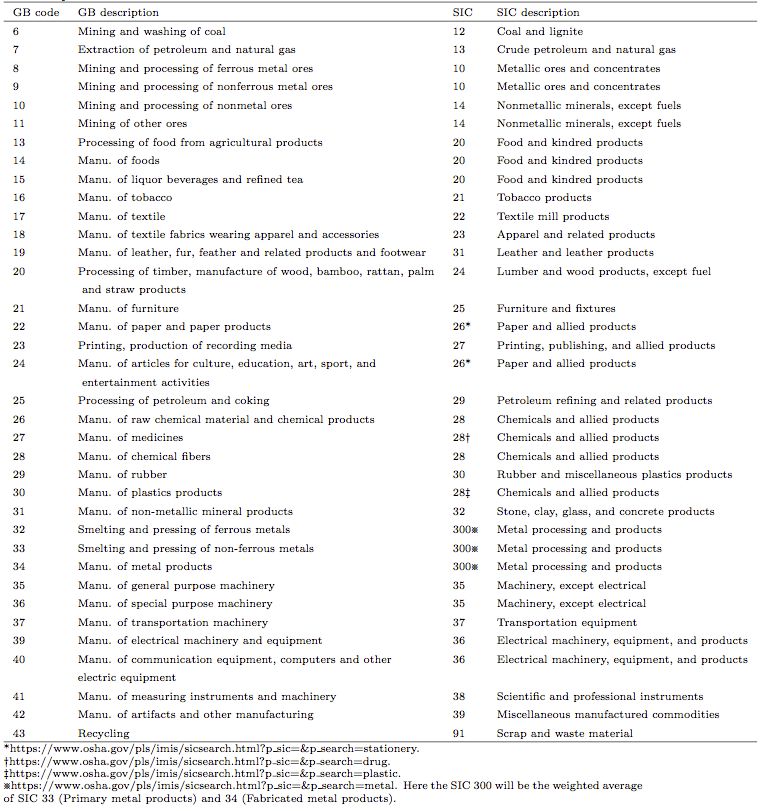
A prefecture’s tariff reduction was uncorrelated with its pre-WTO wage and GDP growth (Tian
2020). We show that empirically, the change in the trade exposure of an origin village from 2001 to
2010 was uncorrelated with changes in the out-migration rate, the share of land leased, the value of
agricultural machinery, and TFP in the 1995–2001 period.
       We first show the impact of an origin village’s trade exposure on rural workers’ occupation choice.
A one-standard-deviation larger decline in destination prefectures’ output tariffs resulted in a three-
percentage-point (or a 0.21-standard-deviation) larger increase in the share of non-agricultural labor
in the origin village. The result is robust to (1) including agricultural trade shocks that could
potentially be correlated with manufacturing trade shocks and affect the agricultural production
directly, (2) using alternative measures of out-migration collected at the village level, (3) controlling
for the initial crop patterns and contemporaneous crop patterns, and (4) controlling for the share of
migrants who moved to the top 10 migrant destinations.8
       The results also imply larger effects for places that were less far along in the process of ur-
banization and agriculture modernization. We find that the effect was larger for villages with less
land per agricultural worker in 2001. The initial land-to-labor ratio in agriculture was positively
correlated with village characteristics that were pro-reallocation, such as the land market fluidity
and the non-agricultural labor share, and was negatively correlated with factors that impeded land
consolidation, such as the ruggedness. Villages with a smaller land-to-labor ratio also had a larger
correlation of the output value and TFP across households, which is a direct measure for allocation
efficiency. Hence, regions with a smaller land-to-labor ratio had larger factor misallocation at the
beginning of the period, and they reacted more strongly to out-migration shocks. This finding is
consistent with the observed irreversibility of urbanization; as pointed out in Lucas [2004], “this
transition is an irreversible process that every industrializing society undergoes once and only once.”
       We then investigate the effect of trade exposure on the rural land market. The land rental market
became more active in the face of the trade shock. A one-standard-deviation larger decline in the
destination prefectures’ output tariffs led to a 26% (or a 0.16-standard-deviation) larger increase in
the stock of land leased, a 76% (or a 0.47-standard-deviation) larger increase in the flow of land
leased within the year, and larger increases in the income from land rental. In addition, the shift
of land from unproductive farmers to productive farms was stronger in villages that experienced
larger shocks. Villages facing a one-standard-deviation larger tariff decline in migrant-destination
prefectures had a 15% larger elasticity of land to TFP at the household level, indicating that the
land allocation efficiency improved more in villages more exposed to the trade shocks.9
   8
      The last exercise intends to address the concern raised in Borusyak et al. [2020] on the how dispersed the migration
network (“shares” in general terms in the shift-share design papers) was and whether the shock-level law of large
numbers applies.
    9
      We measure household-level productivity instead of plot-level productivity since we can only follow households
over time, not plots. An alternative story could be that the plots are heterogeneous in land productivity and TFP
is higher in the most efficient plots. When the outside option of non-agriculture increases, the workers abandon the
village and go to manufacturing, wages in rural areas go up, so the less productive land plots shut down and are
reallocated to more productive plots. This story involves no inefficiency and features Melitz-style reallocation among
efficient producers. Our empirical evidence is not consistent with this story since when farmers move out of the
villages, the land transactions and rents increase instead of decrease.

                                                            4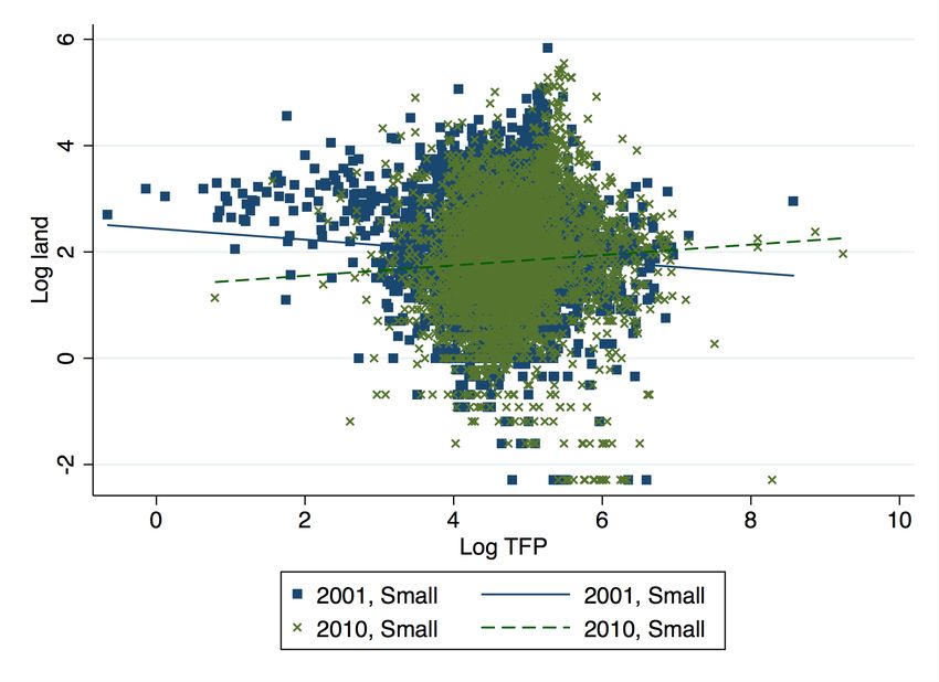
Declines in destination prefectures’ output tariffs encouraged the adoption of agricultural machin-
ery, especially for villages with more between-prefecture migration. There are several explanations
for the increase in agricultural machinery. First, farmers may substitute labor with capital when
labor costs increase (Manuelli and Seshadri 2014). Second, if there are scale-dependent returns to
mechanization due to larger contiguous land areas, farmers may adopt machinery only when the land
size is sufficiently large (Foster and Rosenzweig 2011, 2017). Third, the reduction in land misalloca-
tion can also lead to increased capital adoption, since productive agricultural households are able to
lease in more land and use more capital. Fourth, migrant remittances can ease the household credit
constraint and facilitate capital adoption. We find evidence supporting the first three explanations,
but not the last one.10
    We additionally show that trade shocks increased the output weighted village-level TFP. The
effect came from improved allocation efficiency, with increasingly more output produced by initially
more productive households in villages with larger trade shocks. Migrant selection patterns were
also consistent with the aggregate productivity effects. Using individual-level information from
2003 to 2008, we show that non-agricultural income was positively correlated with factors such as an
individual’s education level and having non-agricultural occupational training, but that these factors
were not good predictors of agricultural productivity. Initially unproductive farming households were
more likely to leave agriculture, and they responded more strongly to the trade shocks.11
    We focus on the output tariff shocks since they generate shocks to pull factors of out-migration for
origin villages; we do not intend to characterize the full impact of the WTO accession on the Chinese
economy. The WTO accession affected manufacturing trade in China through multiple channels,
including the reduction in output tariffs (Tian 2020), reduction in input tariffs (Zi 2020 and Brandt
et al. 2017), and the reduction in trade uncertainty induced by the establishment of the U.S.–China
permanent normal trade relationship (PNTR)(Pierce and Schott 2016; Handley and Limão 2017;
Facchini et al. 2019; and Erten and Leight, Forthcoming). We focus on the reduction in output tariffs
since the output tariff reduction generates intuitive demand shocks to the manufacturing sector. Yet,
when we empirically evaluate the effects of the PNTR shock, we find effects of similar magnitudes
on the land market, capital, and TFP, and insignificant effects on the occupation choice. The PNTR
shock is approximately orthogonal to the output tariff shocks, in the sense that controlling for the
PNTR shock does not affect the coefficient estimates of output tariff shocks (also see Handley and
Limão 2017 and Tian 2020).
    Finally, we present a simple two-sector open-economy model with land market transaction costs
to investigate the role of migrant selection, land market frictions, and sectoral productivity shocks
in determining the patterns of urbanization and agricultural modernization. We calibrate the model
parameters using the NFP Survey data and conduct quantitative exercises. Overall, consistent with
  10
     Overall, the finding on capital adoption is consistent with Hornbeck and Naidu [2014] and Clemens et al. [2018]
with out-migration shocks resulting from natural disasters and labor market policies, respectively. Capital adoption
reinforces the urbanization process: once machines are in place, the production is not likely to revert back to the labor-
intensive mode. Similar transitional paths can be found in the manufacturing sector. See, for example, Acemoglu and
Restrepo [2017].
  11
     We do not find important roles for switching to high-value cash crops or husbandry.

                                                            5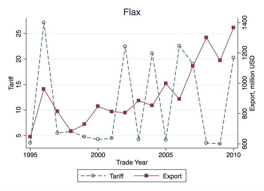
the empirical results, we find a mild positive correlation between an individual’s agricultural and non-
agricultural productivity (0.17). The land market transaction costs were substantial and declined
slightly from 2001 to 2010. In this time period, the economy experienced much faster growth in the
non-agricultural productivity than in the agricultural sector. Despite the large transaction costs in
the agricultural land market, we find that reducing the transaction costs have smaller impacts on
urbanization and agricultural modernization than the growth of non-agricultural productivity.12
    The paper contributes to several strands of literature. First is the literature on structural trans-
formation. Existing research mostly focuses on its initial causes: productivity growth in the agri-
cultural sector (Ngai and Pissarides 2007; Bustos et al. 2016), declines in the prices of agricultural
machinery (Yang and Zhu 2013), and declines in relative cost of obtaining non-agricultural skills
(Caselli and Coleman 2001). To our knowledge, this paper is the first to demonstrate that interna-
tional trade in manufacturing accelerates the development process in agricultural sectors that are
not directly exporters. Second, there is an extensive literature on how land misallocation affects
agricultural productivity. The ambiguity of land rights in developing countries limits land realloca-
tion and creates misallocation (Adamopoulos et al. 2017), and land reforms that clarify land rights
can improve land allocation efficiency and increase agricultural productivity (de Janvry et al. 2015;
Chari et al. 2020). We complement this literature by showing that in addition to the institutional
barriers, the lack of land leasing activity is partially due to the fact that farmers usually do not
have good outside options in non-agricultural sectors. The opportunity to work in the manufac-
turing sector can create a more fluid land market, potentially reducing misallocation. Third, the
existing literature on out-migration of rural residents focuses on its effect on self-insurance (Kinnan
et al. 2018), participation in local risk-sharing networks (Morten 2019), individual migrant outcomes
(Johnson and Taylor 2019), and rural labor markets (Akram et al. 2017; Dinkelman et al. 2017). We
demonstrate that when out-migration is not motivated by income smoothing when facing temporary
shocks, but as a part of the structural transformation, factor markets adjust, leading to productiv-
ity changes. Fourth, the paper contributes to the literature on the impact of international trade
liberalization on the Chinese economy. Most literature discuss the impact of trade liberalization on
manufacturing productivity and exports (Khandelwal et al. 2013; Brandt et al. 2017; Handley and
Limão 2017, among others), migration (Facchini et al. 2019; Zi 2020), sectoral employment shifts
(Erten and Leight, Forthcoming), and reforms in labor institutions (Tian 2020). We show that man-
ufacturing trade affects the development process of the agricultural sector through land reallocation,
capital investment, and worker selection.
    The rest of the paper is organized as follows. Section 2 provides background information on
the land market and the WTO-induced trade shocks in China. Section 3 presents the key data
sources and relevant measurement. Section 4 presents motivating facts linking out-migration to
  12
     Our model follows Adamopoulos et al. [2017] closely, while we explicitly model the source of the land market
misallocation as the transaction cost of leasing. In our model, reductions in the land market transaction cost increase
the land rental price and unproductive farmers leave agriculture, improving the allocation efficiency. Faster growth
in the non-agriculture productivity increases the opportunity cost of remaining in agriculture, and also draws the
unproductive farmers out of agriculture. These mechanisms complement Lagakos and Waugh [2013], where the
subsistence food requirement keeps unproductive farmers in agriculture.

                                                          6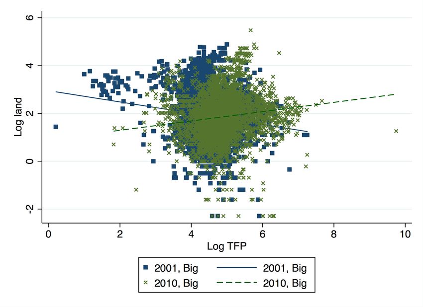
land reallocation and agricultural efficiency. Section 5 shows main empirical findings. Section 6
discusses the selection pattern. Section 7 presents the model and quantitative exercises. The last
section concludes.

2         Background
2.1        The Rural Land Market in China
         Land market conditions are an important aspect of the agricultural sector, since land is an
essential input in agricultural production, and developing countries usually suffer from weak land
right protection. Since the establishment of the Household Contract Responsible System (HCRS) in
the early 1980s, Chinese agricultural land has been collectively owned by the village and contracted
to households within the village commune. The initial land distribution was set mainly based on
household sizes at the time of HCRS establishment. The first round of contracts was set with a
length of about 15 years and they were extended for another 30 years around 1998. Households have
the right to use the contracted land for agricultural production, and the right of leasing the land to
other households within the same village commune was legalized in 1988.13
         However, the rural land market remained very thin before the 2000s. Despite de jure tenure secu-
rity, within-village land reallocation happened, and village leaders had discretion in the reallocation
(Rozelle et al. 2002). In addition, institutions that supported dispute resolution were absent.14 This
insecurity of land rights decreased the incentive of land rental, since households feared that they
could lose their land in the next round of land allocation if they didn’t work on their own land (Ben-
jamin and Brandt 2002; Rozelle et al. 2002; Adamopoulos et al. 2017). If the farmers did not have
stable means of living other than agricultural production, they might not be willing to lease their
land to other households even if other households were more productive, due to the perceived “use
it or lose it” rule. This missing rural land market created misallocation of land across households,
given the initial egalitarian distribution rule.
         The land leasing market became more active alongside with urbanization, since the opportunity
cost of remaining in crop farming became higher. According to decennial population censuses, the
share of population living in urban areas increased from 26% in 1990 to 36% in 2000, and then to
50% in 2010. Meanwhile, the share of households with land lease income increased from about 4%
in the 1990s to 12% in 2010.15

2.2        Internal Migration and the WTO Shock
         Urbanization came alongside with large flows of internal migration. The Chinese household
registration system, i.e., the Hukou system, assigns all residents with a prefecture-sector-specific
    13
     See the full description of timing of the reforms in Appendix A.2.
    14
     The Law of the People’s Republic of China on the Mediation and Arbitration of Rural Land Contract Disputes
was enacted in 2010. Before that, several regulations issued by the central government tried to address the issues of
contract disputes starting from 1992.
  15
     Calculated using the NFP Survey.

                                                         7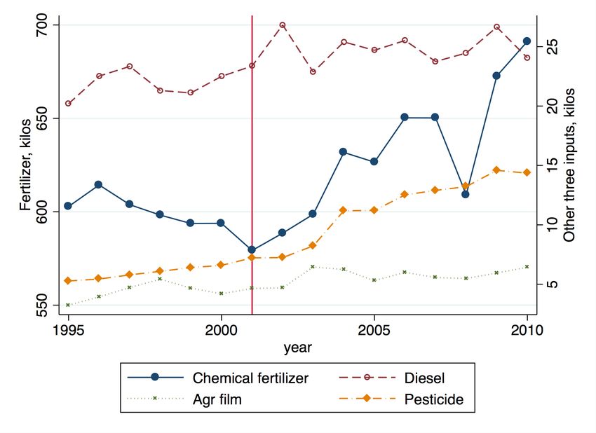
registration status, where a sector is either agriculture or non-agriculture. A person is an internal
migrant when living and working in a prefecture-sector different from their registration. In 2000,
11% of the population were migrants, and the number increased to 20% in 2010. Migration is closely
tied with sectoral employment shifts: 93% of migrants work in the non-agricultural sector.16
       China’s accession to the WTO was an important driver of the fast growth in the manufacturing
sector and increased internal migration (Brandt et al. 2017, Zi 2020, Facchini et al. 2019, and Tian
2020). The WTO accession reduced international trade barriers, with the average tariff on Chinese
exports declined from 3.7% in 2001 to 2.4% in 2010 (Figure 1, the line with solid dots). The average
tariff is the weighted average across industries, using industry export values as weights. Industry
level tariffs are calculated as the weighted average of tariffs on Chinese exports imposed by importing
countries, using the 2001 export values as weights.17 Manufacturing exports from China increased
from less than 400 trillion dollars in 2001 to 1,750 trillions in 2010 (Figure 1, the line with hollow
diamonds). This substantially increased demand for labor in the manufacturing sector, and resulted
in increased internal migration (Tian 2020).18

                                              [Figure 1 about here.]

       Regions varied in the extent of the export demand shock based on their initial industrial com-
position, since the size of tariff reductions were different by industry. Figure 2 uses the 2001–2010
change as an example to show the variation in tariff reductions and export growth by industry.
Similar to Tian [2020], we use the reduction in output tariffs on Chinese exports to measure the
WTO shock. The reduction in tariffs was due to China’s eligibility of the Most-Favored-Nation
status, and a reduction in the output tariff effectively increased the output price. Empirically, the
industry-level tariff changes in the post-WTO period (2001–2007) were uncorrelated with export
growth and tariff changes in the pre-WTO period (1995–2001). We measure the prefecture-level
tariff reductions as the weighted average of industry-level tariffs, using industry-level employment
shares as weights. The prefecture-level tariff reductions in the post-WTO period were uncorrelated
with pre-WTO wage and GDP growth.

                                              [Figure 2 about here.]

       Additionally, one might be concerned that the agricultural sector faced tariff changes on its
output that were correlated with manufacturing sector tariff changes. Overall, the WTO’s direct
impact on the agricultural goods market is less clear. China’s import tariff on soybeans declined
from over 100 percentage points to zero, and soybean imports increased from less than 5 trillion
  16
     Calculated using the 2000 and 2010 population census.
  17
     The export elasticity with respect to tariffs can be estimated using a panel regression of log exports on tariffs
on the industry-year level, with industry fixed effects and year fixed effect. The elasticity estimate is 0.074 using 26
two-SIC code industries and 2001–2010 data. It indicates that a one-percentage point decline in the output tariff is
correlated with a 7.4% increase in exports.
  18
     In addition, Tian [2020] shows that regions with more favorable export shocks started to provide more amenities
for migrant workers, and these changes further increased the incentive to migrate.

                                                          8
dollars in 2001 to 25 trillion in 2010. For other crops, however, imports and exports fluctuated over
time, and there were no clear patterns of tariff changes.19

3     Data and Measurement
3.1    Occupation Choice and Migration
    In order to measure a rural resident’s occupation choice and production activities, we use the
NFP Survey, a longitudinal survey conducted by the Research Center for the Rural Economy under
the Ministry of Agriculture in China. The survey started in 1986 and continues until now. Multi-
stage sampling is used to get a nationally representative sample of around 300 villages and 20,000
households per year. Households and villages are followed with little attrition and are added over
time for representativeness.20 The core module of the household questionnaire remains stable, with
household-level demographic summaries, agricultural production, assets, income, and expenditure.
We use the 2001–2010 data for the main analysis of the post-WTO period and 1995–2001 data to
check pre-trends.21 Our main analysis is based on the household-level information and village-level
measures aggregated from household data, and we supplement it with the village questionnaire and
individual questionnaire.22 An administrative village or subdistrict is the lowest level of government
administration in China, with county, prefecture, and province as successively more aggregate levels
of government.
    One key element of our analysis is the definition of a rural resident’s occupation. There are
broadly three categories: laborer, entrepreneur, and public-sector employee. We focus on laborers
who are wage earners: they are employed outside their own household and work for wages.23 Thus,
a wage earner can be (1) working in his own village and employed by other households, (2) employed
by firms in his own village, (3) working outside the village, but within the same prefecture, or (4)
working in a different prefecture.24
    Empirically, Case (1) is not prevalent in rural China: hired labor days is on average only 2%
of total labor days in any family operations, during the 2001–2010 period. The share of Type (2)
workers is also likely to be small. According to the individual-level data between 2003 and 2010, a
wage earner spends 212 days working outside the village on average. Thus, the majority of the wage
  19
     Oil crop, flax, vegetable and fruit experienced large increases in the value of import, although the scale was much
smaller than soybean. See trade and tariff trends of major crops in Appendix B.5. In Appendix D.5, we show that
our main results are robust to controlling for agricultural trade shocks.
  20
     We provide evidence on the absence of selective attrition in Appendix B.2.1.
  21
     The data is not available in 1992 and 1994. After 2003, demographic informations are collected at the individual
level, and production information is more detailed, with inputs and outputs information by crop.
  22
     The survey intends to get an accurate and consistent picture of agricultural production and rural household life for
the support of policy making. For details of the survey disclosed by the survey center, see http://jiuban.moa.gov.
cn/sydw/ncjjzx/gcdgzdt/gzdtg/201302/t20130225_3225848.htm. Also see Benjamin et al. [2005], Banerjee et al.
[2012] for other descriptives of the data.
  23
     Entrepreneurs are managers of firms and businesses. Public-sector employees include teachers, medical workers,
and civil servants.
  24
     A prefecture is composed of rural villages and village-equivalent urban units (town and districts). See the Chinese
administrative units in Appendix B.1. There are 333 prefectures, and each prefecture has about 2200 villages.

                                                           9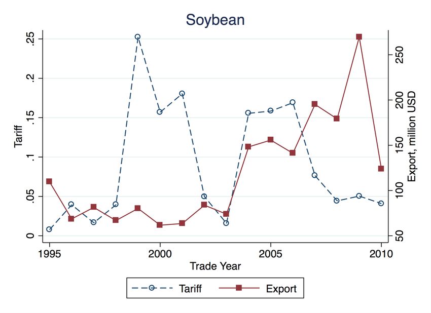
earners are working outside the village, either in the urban areas of their own prefecture, or in other
prefectures. In addition, the wage earners are predominantly working in non-agriculture. As shown
in Appendix B.3 using the individual-level data between 2003 and 2010, 97% of the wage earners
work in the non-agriculture sector.
       Our main measure for the occupation choice is the non-agricultural labor share of a village, and
it is the ratio of the total number of wage earners to the total number of labor in a village, where
both numbers are aggregates from the information in the household questionnaire (Table 1). The
village questionnaire has information on the number of laborers outside the village and decomposes
the number into within-county, between-county, and between-provinces; we use the information in
the robustness checks.25

                                              [Table 1 about here.]

       In order to measure pre-existing migration connections between prefectures, we use the 0.095%
individual sample of the 2000 census to construct the prefecture-to-prefecture migration network.
The census has information on the residence prefecture in 2000 and the residence prefecture in 1995
(Table 1). Thus, we know the number of people who lived in prefecture i in 1995 moved to prefecture
j before 2000 (mij ).26
       We also use the census to construct the share of cross-prefecture migrants out of all migrants. The
share of cross-prefecture migrants is relevant for our analysis, since an origin village’s exposure to
other prefectures’ trade shocks is larger if initially, a larger share of the village residents were working
in those prefectures. The total number of cross-prefecture migrants from prefecture i is mbetween
                                                                                               i      ⌘
P
   j6=i mij . The within-prefecture migrants are identified using the question on the registration place
of Hukou. A person is defined as a within-prefecture migrant if his Hukou registration is in the same
prefecture, but in different counties. Denoting the number of within-prefecture migrants as mwithin
                                                                                            i      ,
we calculate the share of cross-prefecture migrants as

                                                        mbetween
                                                          i
                                            si =                      .
                                                   mbetween
                                                    i       + mwithin
                                                                i

       Given that prefecture is the finest geographical unit we can get for the migration information,
we make the assumption that all villages (v) in a prefecture (i) shares the same migration network
that connects other prefectures. If this assumption is violated, it will drive the empirical results
toward zero. We also assume that the propensity of cross-prefecture migration is the same for all
villages within a prefecture. Thus, sv(i) = si for all villages (v) in a prefecture (i).27
  25
     The village questionnaire is filled by village heads, and we think the village-level aggregates from household
questionnaires are of higher quality, which are what we use in the main analysis.
  26
     See Appendix C for descriptives of the migration network.
  27
     If this assumption is violated, we have measurement errors in the village-to-prefecture migration network. If the
measurement error is classic, the exposure to trade shock will be measured with error, and the effect of trade exposure
on the outcomes will be biased toward zero.

                                                         10
3.2 Regional Trade Shocks
We first construct the prefecture-year level trade exposure in the manufacturing sector. The
output tariff (⌧ ) on exports faced by prefecture i is calculated using applied tariffs from the World
Bank TRAINS dataset on the 2-digit SIC level in the manufacturing sector. The output tariff on
exports is the weighted average of tariffs on Chinese exports imposed by importing countries, with
their 2001 import values as weights. Following Kovak [2013], the regional output tariff in prefecture
i and in year t is
X
⌧ it = ik ⌧kt,
k
1
ik ✓ik
where ik =P 1 , (1)
k0 ik0 ✓
ik0
ik = P Lik is the fraction of regional labor allocated to industry k, and 1 ✓ik is the cost share
k0 Lik0
of labor in industry k. ik and ✓ik are calculated using the 2000 Industrial Enterprises Survey data,
and only manufacturing industries are included.28 ⌧kt is the industry-year-specific tariff. A village
v’s (in prefecture i) exposure to its own prefecture’s output tariff is
own
⌧v(i)t = ⌧it . (2)
Accordingly, its exposure to tariffs in other prefectures is
X mij
other
⌧v(i)t ⌘ P ⌧jt , (3)
j6=i j 0 6=i mij 0
where mij is the number of people who are in prefecture i in 1995 and reside in prefecture j in 2000.
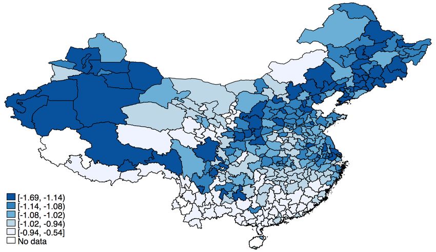
Figure 3 shows the geographic distribution of own prefecture’s output tariff reduction and other
prefectures’ output tariff reduction, using the 2001–2010 change as an example. Panel (a) shows
the distribution of own prefecture’s output tariff reduction, defined as ⌧2010
own own , and Panel (b)
⌧2001
shows the distribution of other prefectures’ output tariff reduction, ⌧2010
other other . Darker colors
⌧2001
represent larger reductions. We can see that the distributions are different for the two types of tariff
reductions. The declines in own prefecture’s output tariff ranged from –3.96 to –0.14 and were rather
scattered across the country. The declines in other prefectures’ output tariff ranged from –1.69 to
–0.54 and were larger in northern China.
[Figure 3 about here.]
28
The 2-digit industry codes in the survey is different from the SIC code, and we provide concordance in Appendix
B.4.
113.3 Total Factor of Productivity (TFP) Estimation
Household TFP In order to track the allocation of land across households with different produc-
tivity levels, we construct household-level TFP. We estimate household-level revenue TFP instead
of quantity TFP due to data constraints. Crop outputs are available in all years in quantities (ki-
los), but the input data varies by year. There are four types of inputs in crop farming: land (in
hectares), labor (in labor days in agriculture), capital (in initial book value), and intermediate inputs
(in value, including seed and seedlings, fertilizers, agricultural films, and pesticides). In our main
analysis, we aggregate across crops to generate household-level outputs and inputs to estimate the
household-level TFP.
The output value is constructed using a common vector of year-specific crop prices and household-
level crop outputs. We include 11 types of crops that are consistently measured in the data: wheat,
rice, corn, soy bean, cotton, oil crops, sugar crops, flax, tobacco, fruits, and vegetables.29 For each
crop, we calculate the sales price in yuan per kilo for all households with positive sales. The price
of a crop in a particular year is calculated as the national average of all households. Then the
household-level output is the sum of crop physical outputs evaluated at the common national prices.
We deflate the household level output using the national output price indices to make output values
comparable across years, using 1995 as the baseline year.30,31
We also make adjustments on the input side. The intermediate input value is the total value
of inputs in all crops, deflated by province-level agricultural input price indices, using 1995 as the
baseline year. The capital stock is recorded in initial book value. To take into account differential
prices across years, depreciation of capital stock, and missing values of capital in some observations,
we use the perpetual inventory method to reconstruct the capital stock at the household level.32
Assuming that agriculture production in crop farming follows a Cobb-Douglas form, we estimate
the production function using the following equation:
log(yh(v)t ) = ↵ log(dh(v)t ) + log(kh(v)t ) + log(lh(v)t ) + log(mh(v)t ) + h(v)t , (4)
where yh(v)t is the output value in crop farming in household h, village v, and year t. Labor days in
agriculture, capital, land, and intermediate inputs are dh(v)t , kh(v)t , lh(v)t , and mh(v)t , respectively.
Cobb-Douglas parameters ↵, , , and represent output elasticities with respect to each input,
and are assumed to be constant over time and across households. We further decompose the log of
TFP as follows:
29
Crop area of these 11 crops comprises 90% of total areas in our data, both as the sample mean for households and
as the aggregate share. Other crops that do not show up in all years include potato, mulberry, tea, herbal medicine.
30
The national output price deflator is the price index of crop farming from the National Statistics Yearbook of
Agriculture. We use the national price deflator instead of province-level price deflators since the latter is only available
after 2003.
31
We use common prices to eliminate the price variation across households. In addition, we want to evaluate a
household’s output value even in the absence of crop sales, since the household may consume the output for food or
for livestock feed.
32
See the details of the method in Appendix B.2.3.
12h(v)t = vt + h + eh(v)t .
Here, a household’s productivity in a given year is comprised of factors common to its village in
the year, vt , such as weather and other aggregate shocks, its intrinsic ability to farm and other
time-invariant household-level factors, h, and idiosyncratic shocks, eh(v)t .
We estimate Equation 4 controlling for village-year ( vt ) fixed effects and household ( h) fixed
effects.33 The log of household TFP is measured as the following residual term,
ˆh(v)t ⌘ log(yh(v)t ) ↵
ˆ log(dh(v)t ) ˆ log(kh(v)t ) ˆ log(lh(v)t ) ˆ log(mh(v)t ). (5)
Village TFP We are interested in measuring the village-level TFP since it is informative about the
overall productivity of the village and reflects the efficiency of local land allocation, an important
aspect of agricultural modernization. The village-level productivity ( vt ) is constructed as the
weighted average of log household TFPs, using the output value (yh(v)t ) as weights,
X X yh(v)t
vt ⌘ wh(v)t ˆh(v)t = P ˆh(v)t . (6)
h h h0 yh0 (v)t
In addition, similar as in Chari et al. [2020], we decompose the village-level TFP in the following
way,
X
vt = vt + (wh(v)t wvt )( ˆh(v)t vt ) ⌘ vt + Evt , (7)
h
P ˆ P
where vt ⌘ 1
Nh h h(v)t and w̄vt ⌘
1
Nh h wh(v)t = 1
Nh represent unweighted means, with Nh as
the number of households in the village-year. The second term Evt is the sample covariance between
the household-level output weights and productivity multiplied by Nh 1. A larger Evt indicates
that the productive household generate more output and have a larger weight in the calculation of
the village-level TFP. Thus, we use it as one measure of allocation efficiency.
4 Key Motivating Facts
4.1 Less Labor, More Land Rental, More Capital, Higher Land and Labor Pro-
ductivity in the Agricultural Sector after 2001
We first present the trends of labor, land, capital markets for the 1995–2010 period, with trend
breaks around 2001. First, more and more households moved out of crop farming and started to
33
See the details of the TFP estimation in Appendix D.2. The estimates for the output elasticity of inputs are
similar as in Chow [1993], Cao and Birchenall [2013], and Chari et al. [2020]. An alternative method is to use the
log value-added as the outcome variable (the output value minus the intermediate input value), and the estimated
TFP is denoted as ˆVhvt . To alleviate the concern that the input choices are correlated with unobserved idiosyncratic
productivity shocks, we use the lagged inputs as instruments for the inputs in the current period. The TFP estimates
with the IV method are very similar to the OLS estimates, so we use the OLS estimates directly.
13work for wages (Figure 4 Panel a). The share of households whose main business were crop farming
declined from 79% in 1995 to 75% in 2001, and further declined to 66% in 2010. This decline
is mirrored by the increase in the share of households where the entire household worked in non-
household business: while the 1995 to 2001 change was less than 2%, the share increased by 5%
afterwards.34
The land rental market became active mostly after 2001 (Panel b). Less than 5% of households
had income from land leasing between 1995 and 2001, and the number increased to 13% in 2010.
The size of land-lease income also grew a lot in the post-2001 period, from 550 yuan per household
to 2500 yuan in 2010.35
[Figure 4 about here.]
Alongside the outflow of labor and land rental activities, the amount of capital increased. The
dotted line in Panel (c) shows that the average value of total capital stock for households in agricul-
ture increased from 4.8 thousand yuan in 2001 to eight thousand yuan in 2010, with a much smaller
change before 2001. Similarly, the value of agricultural machinery had an increase of one thousand
yuan after 2001, while the before 2001 changes was less than 0.5 thousand yuan.36
The patterns of labor and land productivity growth in Panel (d) were consistent with the in-
creased capital input. Land productivity is defined as the log kilos per hectare, and labor produc-
tivity is the log kilo per labor day in agriculture. Take wheat as an example, the land productivity
remained relatively stable before 2001 and experienced a 0.3 log-point increase afterwards, and the
increase of labor productivity was 0.8 log-point after 2001.37
Overall, we find that the agricultural sector experienced outflow of labor, increased land rental
activities, more capital adoption, and higher land and labor productivity through the 1995–2010
period, and the change was accelerated after 2001.
4.2 Tariff Reductions Led to Increases in Internal Migration
We argue that the outflow of labor from agriculture was closely related to the fast growth of
manufacturing exports after 2001. Our main analysis focuses on how increased trade exposures in
34
Households can be either in the family-run business or in non-household business. Family-run business uses
households as the unit of operation, relies entirely or mainly on household members’ labor supply, utilizes family-owned
or contracted factor inputs, directly organizes the production, does accounting independently, and bears its own gains
or losses. There are eight categories for the family-run business: crop farming, forestry, husbandry, manufacturing,
construction, transportation, service.
35
Appendix D.1 shows that household occupation choices were correlated with how much land they decided to work
on. In a household with three laborers, the probability of working on any land was six percentage points smaller
when one more household member worked as a non-agricultural laborer; conditional on non-zero land in agricultural
operation, the land size was 25% smaller.
36
Capital in all years are valued at 1995 yuan using the perpetual inventory method (see Appendix B.2.3 for details).
There are eight types of capital in the survey: draft animals, hand farm tools valued at least at 50 yuan, agricultural
machinery, industrial machinery, transportation machinery, facilities, fixed infrastructure, and other.
37
On average, a household had 0.5 hectare land in 2001 and 0.48 hectare in 2010. In comparison, a household had
1.8 agricultural laborers in 2001 and 1.3 in 2010. Given the outflow of labor and relative stable total agricultural land,
it is reasonable for the labor productivity to increase more than the land productivity. Appendix B.6 shows that the
trends were similar for rice, corn, and soybean.
14migration destinations pulled labor out of villages, i.e., from sending regions’ perspective. Here, we
first provide a mirror evidence from receiving regions’ perspective, i.e., how the declines in the output
tariff in a region pulled in labor. In Figure 5, each dot is a prefecture. The horizontal axis is the
change in output tariffs from 2000 to 2010 (⌧2010
own own ), and the vertical axis is the change in the
⌧2001
share of migrants, calculated using the 2000 and 2010 censuses. The slope is -0.016 and statistically
significant at the 5% level, indicating that a one-percentage point larger decline in output tariffs in
export markets resulted in a 1.6 percentage point larger increase in the share of migrants.
[Figure 5 about here.]
4.3 Larger Trade Shocks, Larger Correlations between Land and TFP within a
Village
We show that the land allocation efficiency increased in villages with bigger trade shocks. In
Figure 6, we split the villages into two group using the size of the trade shock they experienced from
2001 to 2010. The 2001 to 2010 trade shock is defined as the difference between a village’s exposure
to other prefectures’ output tariff in 2001 and 2010, i.e., (⌧2010
other other ) ⇥ s, where s is the share of
⌧2001
cross-prefecture migrant share. The shocks larger than the median magnitude (in absolute values)
are defined as large shocks, and the shocks smaller than the median are defined as small shocks.
Panel (a) shows the correlation between the log land and log TFP for households in the villages with
small shocks. In 2001, the slope was -0.10, indicating that households that had larger productivity
worked on smaller land (the squares and the solid lines). The slope became 0.10 in 2010, which
suggests an improvement in land allocation efficiency (the crosses and the dashed lines). However,
the increase was bigger for villages that experienced an above-median trade shock: the slope was
-0.24 in 2001 and increased to 0.19 in 2010 (Panel b).
[Figure 6 about here.]
In sum, we find evidence that the Chinese agricultural sector experienced large changes after
2001, and the change was connected to the reductions in output tariffs in the manufacturing sector.
We formally investigate this hypothesis in the next section.
5 Main Empirical Results
5.1 Village-Level Results with Trade Shocks: Empirical Specification
Our empirical analysis intends to show the impact of trade shocks on various outcomes in the
agricultural sector. The baseline estimation equation is as follows:
other other own own
yvt = 0 + ⌧v(i)t + ⌧v(i)t + Xvt + Ipt + Iv + ✏vt , (8)
where yvt is the outcome variables, including the share of non-agricultural labor, various measures of
land, the log of agricultural machinery value, and the village-level TFP in village v and year t. ⌧v(i)t
own
15and ⌧v(i)t
other are village v’s exposure to its own prefecture i’s tariff and other prefectures’ output tariff,
respectively. We include a matrix of controls Xvt , including the log total number of laborers, the log
total number of households, and the log government transfers plus one. Province-year fixed effects
Ipt are controlled for to take into account unobserved province-year specific weather conditions and
various government policies that potentially affect sectoral employment choices and land allocation
rules.38 Village fixed effects Iv control for all time-invariant village characteristics such as overall
land quality, climate, other agro-geographical characteristics, and social norms regarding migration
and land allocation. Standard errors are clustered at the province level and at the year level to take
into account correlated shocks within provinces and within years.
other and own are the reduced-form parameters of the impact of tariffs on agricultural pro-
duction. A reduction of output tariffs in the manufacturing sector effectively increases the price of
goods received by exporters. Thus, wages in the manufacturing sector increase, and it acts as a pull
factor for labor to move out of the agricultural sector. Both the trade shocks in one’s own prefecture
and other prefectures can impact the sectoral employment choices. other and own being negative
means that lower output tariffs on manufacturing goods in export markets increase yvt .
Our main parameter of interest is other . If both the own prefecture’s output tariff and other
prefectures’ output tariff affect the agricultural production only through the labor market, we expect
declines in either one leading to increased outflow of labor from agriculture. However, manufacturing
trade can also affect agricultural production through other channels. For example, the positive shocks
to manufacturing trade increase the income of urban residents, and the increase in income leads to
higher demand for agricultural goods with larger income-elasticities. Then agricultural production
is affected by the manufacturing growth through the agricultural goods market. If we assume that
the agricultural goods market is relatively local, then we expect such demand effects to be captured
in own rather than in other . In other words, we think that other is more likely to capture the
labor demand effect.39
The key identification assumption is that the counterfactual changes in the outcome variables are
the same across villages in the absence of trade shocks. Since the counterfactual is not observed, we
use pre-trends to provide suggestive evidence on the exogeneity of trade shocks. The hypothesis is
that there were no village-level trends in the share of non-agriculture labor, land rental, agricultural
capital, and TFP before 2001 that were predictors of post-2001 changes in ⌧v(i)t
own and ⌧ other . We test
v(i)t
this hypothesis empirically by running the following regression,
o o
⌧v(i)t = o + 1 ⌧v(i)2001 + ⇧Zv1995–2001 + Ip + ⇠v , (9)
where o = own, other, t = 2002, ..., 2010, and Zv1995 2001 is a vector of changes of village-level
variables from 1995 to 2001, including changes in the share of non-agriculture labor, land rental,
agricultural capital, and TFP, and Ip are province fixed effects. We find no evidence of differential
38
For example, Chari et al. [2020] shows that provinces implemented the 2003 national land contract law at different
times.
39
In general, prefecture-to-prefecture goods trade and migration can still be correlated due to common costs, such
as transportation.
16trends of key outcome variables for villages with different sizes of trade exposures. The results are
shown in Appendix D.4.
Our second main specification takes into account that regions differ in their share of cross-
prefecture migrants sv(i) out of all migrants. The impact of pull factors of cross-prefecture migration
is larger if in the beginning of the period (2000), a larger share of people moved across prefectures
rather than within prefectures. In other words, sv(i) intensifies the impact of other prefectures’
output tariff on the origin village’s tendency to leave agriculture. Thus, our second main specification
adds an interaction term of other prefectures’ output tariff ⌧v(i)t
other and the share of cross-prefecture
migrants sv(i) ,
other other inter other own own
yvt = 0 + ⌧v(i)t + ⌧v(i)t ⇥ sv(i) + ⌧v(i)t + Xvt + Ipt + Iv + ✏vt , (10)
and we expect the coefficient inter to be negative.
5.2 Village-Level Results with Trade Shocks
Occupation Choice We first investigate the impact of output tariffs on the occupational choice
for rural residents in Table 2. Column (1) regresses the share of non-agricultural labor on other
prefectures’ output tariff, controlling for province-year fixed effects and village fixed effects. The
coefficient for other prefectures’ output tariff is -0.08 and significant at the 1% level, indicating
that a one-standard-deviation larger decline in other prefectures’ output tariff resulted in a 3.5-
percentage-point (or a 0.25-standard-deviation) larger increase in the share of non-agricultural labor.
Column (2) adds own prefecture’s output tariff, and the coefficient of other prefectures’ output tariff
becomes smaller and statistically significant at the 1% level. Column (3) follows the specification
in Equation 8, adding the village-year specific controls (i.e., the log total number of laborers, the
log total number of households, and the log government transfers plus one). The coefficient for
other prefectures’ output tariff remains stable. Column (4) follows the specification in Equation 10,
adding an interaction of other prefectures’ output tariff with the share of cross-prefecture migrants.
The coefficient for the interaction is indeed negative as expected, indicating that villages with larger
share of cross-prefecture migrants were impacted more strongly by other prefectures’ trade exposures.
Overall, we find that trade shocks in other regions pulled labor out of agriculture; more so for villages
with higher shares of cross-prefecture migrants.
[Table 2 about here.]
We also find heterogeneous effects of other prefectures’ output tariff with respect to the initial
land-to-agriculture-labor ratio. Column (5) interacts others prefectures’ tariff with the log agricul-
tural land-to-labor ratio in 2001. The coefficient for other prefectures’ output tariff is –0.16, and
the interaction term is 0.05. The positive interaction means that for villages with a larger land-to-
labor ratio in agriculture, the effect of a decline in other prefectures’ output tariff was smaller. This
message is clearer in Column (6), where we interact other prefectures’ output tariff with quintile
17indicators of a village’s land per agricultural worker in 2001. For villages with the smallest land per
agricultural worker in 2001 (i.e., in the first quintile), a one-standard-deviation larger decline in other
prefectures’ output tariff led to a 8-percentage-point larger increase in the share of non-agricultural
labor. For villages in the fifth quintile, the effect was 3 percentage points.40
We interpret the heterogeneous effect of other prefectures’ output tariff with respect to the land-
to-labor ratio as capturing the role of the extent of factor misallocation at the beginning of the
period. In villages with more active land markets, land is likely to be allocated more efficiently
across households according to their productivity, which allows workers with comparative advantage
in non-agriculture to move out of agriculture. This is also related to the process of urbanization in
general. In regions where the urbanization already took place and people moved out of agriculture,
additional shocks to out-migration had smaller impacts.
This interpretation is supported by the descriptive evidence in Table 3. We regress different
measures of baseline village characteristics in 2001 on the log land per agriculture worker, controlling
for province fixed effects. Columns (1)–(3) use direct measures of land market fluidity as the outcome
variables, and the size of land leased is positively correlated with the log land per agricultural worker.
There are two measures for the land leased. The stock measure comes from the decomposition
of the total land at the end of the year, and the flow is a separate measure on how much land
a household leased during the year. Column (4) shows that a village’s ruggedness is negatively
correlated with the land-labor ratio. An explanation is that land consolidation is harder for villages
with more rugged surface, thus land reallocation is limited.41 Column (5) indicates that the share
of non-agriculture labor is positively correlated with the land-labor ratio. Column (6) provides the
most direct evidence: the allocation efficiency (Ev2001 , which is the covariance between output and
productivity) is positively correlated with the land-labor ratio.
[Table 3 about here.]
The coefficient estimate for own prefecture’s output tariff is positive in all column in Table 2,
indicating that a reduction in own prefecture’s output tariff led to smaller labor outflows from agri-
culture. The positive estimates of the own prefecture’s output tariff impact suggest that there could
be alternative channels through which trade shocks affected the non-agricultural labor share. One
potential channel is through the local demand for agricultural goods. A reduction in manufacturing
output tariffs in prefecture i increased the wage, and the income effect could lead to higher demand
for agricultural goods, especially food such as dairy products, vegetables, and fruits. Thus, it could
be more profitable for farmers to stay in agriculture. We find evidence in Appendix D.10 on how
an increase in own prefecture’s trade exposure led to an increase in the revenue share of cash crops,
although the effect is not statistically significant.
40
Note that the sample sizes are different in Columns (1)–(4) and Columns (5)(6) since not all villages in the
2001–2010 sample show up in the 2001 sample. When we use the 1971 village-year observations to run the baseline
regression as in Column (1), the coefficient for other prefectures’ output tariff is -0.09, which is in between of -0.16
for the first-quintile villages and -0.06 for the fifth-quintile villages.
41
The ruggedness data is from Nunn and Puga [2012] with cells on a 30 arc-seconds grid. The cell-level data is
aggregated to the county level, and our assumption is that villages within a county have the same ruggedness level.
18You can also read