Finite slip models of the 2019 Ridgecrest earthquake sequence constrained by space geodetic data and aftershock locations

Finite slip models of the 2019 Ridgecrest
earthquake sequence constrained by space geodetic
 data and aftershock locations
Zeyu Jin and Yuri Fialko

Institute of Geophysics and Planetary Physics, Scripps Institution of Oceanography,
University of California, San Diego, La Jolla, CA 92023, USA
Corresponding author:
Zeyu Jin
email: zej011@ucsd.edu

Abstract
The July 2019 Ridgecrest, California earthquake sequence involved two large events,
the M6.4 foreshock and the M7.1 mainshock that ruptured a system of intersecting
strike-slip faults. We present analysis of space geodetic observations including Syn-
thetic Aperture Radar (SAR) and Global Navigation Satellite System (GNSS) data,
geological field mapping, and seismicity to constrain the sub-surface rupture geometry
and slip distribution. The data render a complex pattern of faulting with a number
of sub-parallel as well as cross-cutting fault strands that exhibit variations in both
strike and dip angles, including a “flower structure” formed by shallow splay faults.
Slip inversions are performed using both homogeneous and layered elastic half space
models informed by the local seismic tomography data. The inferred slip distribution
suggests a moderate amount of the shallow coseismic slip deficit. The peak moment
release occurred in the depth interval of 3-4 km, consistent with results from previous
studies of major strike-slip earthquakes, and the depth distribution of seismicity in
California. We use the derived slip models to investigate stress transfer and possi-
ble triggering relationships between the M7.1 mainshock and the M6.4 foreshock, as
well as other moderate events that occurred in the vicinity of the M7.1 hypocenter.
Triggering is discouraged for the average strike of the M7.1 rupture (320 deg), but
encouraged for the initial orientation of the mainshock rupture suggested by the first
motion data (340 deg.). This lends support to a scenario according to which the earth-
quake rupture nucleated on a small fault that was more optimally oriented with respect
to the regional stress, and subsequently propagated along the less-favorably oriented
pre-existing faults, possibly facilitated by dynamic weakening. The nucleation site of
the mainshock experienced positive dynamic Coulomb stress changes that are much
larger than the static stress changes, yet the former failed to initiate rupture.

Introduction
The 2019 Ridgecrest, California earthquake sequence initiated on July 4 with a strong
Mw 6.4 foreshock followed by a Mw 7.1 mainshock on July 5. The Mw 7.1 (hereafter, we
drop the subscript w and refer to the earthquake magnitude as to the moment magni-
tude, unless otherwise noted) mainshock was the largest event that struck California

 1

over the last 20 years, since the 1999 Hector Mine earthquake (Barnhart et al., 2019;
Chen et al., 2020; Liu et al., 2019; Ross et al., 2019). The epicentral area of the 2019
earthquake sequence is located between the town of Ridgecrest to the south-west, the
Searles Valley to the east, and the Garlock fault to the south (Figure 1). Faults that
produced the foreshock and the mainshock, as well as their numerous aftershocks, were
not previously recognized as continuous connected features capable of producing a ma-
jor earthquake, but appear to be spatially associated with the Little Lake fault zone.
The latter is in turn part of the Eastern California Shear Zone (ECSZ), a complex
network of active Quaternary faults that accommodates between 10 and 20% of the
relative motion between the Pacific and North American plates (Dokka and Travis,
1990; McClusky et al., 2001; Sauber et al., 1986; Tymofyeyeva and Fialko, 2015). It
has been proposed that the ECSZ represents an incipient plate boundary forming in
response to the development of a major restraining bend in the San Andreas fault
system to the west (Nur et al., 1993). Indeed, all of the major (M 7+) earthquakes
that occurred in southern California over the last 50 years were located in the ECSZ
(e.g., Fialko, 2004; Fialko et al., 2001; Hauksson et al., 2002; Sieh et al., 1993; Simons
et al., 2002).
 The M6.4 foreshock activated a left-lateral northeast (NE) trending fault, and
possibly a 10-20 km long segment of a right-lateral NW trending fault that was sub-
sequently ruptured by the M7.1 mainshock (e.g., Ross et al., 2019). The mainshock
nucleated ∼ 15 km to the NW of the foreshock epicenter and bilaterally propagated
along a system of previously mapped and unmapped right-lateral faults striking NW.
Most of the M7.1 rupture occurred within the boundaries of the US Naval Air Weapons
Station (NAWS) at China Lake. The most recent (prior to 2019) activity in the Ridge-
crest area involved a series of moderate to strong earthquakes in 1995-1996 (Hauksson
et al., 1995), some of which occurred within just a few kilometers from the epicenter
of the mainshock of the 2019 sequence. This clustering of seismic activity, combined
with large volumes of high-quality observations, makes the Ridgecrest sequence a good
target for investigations aimed at improving our understanding of the mechanisms of
spatio-temporal earthquake clustering, stress-mediated earthquake interaction, and
triggering. In this paper we use a rich combination of space geodetic, geologic, and
seismic observations to derive finite slip models of the 2019 foreshock-mainshock se-
quence. We then apply these models to investigate the role of static and dynamic
stress changes and stress heterogeneity in the earthquake triggering.

Data and Methods
The 2019 Ridgecrest earthquakes occurred in the middle of dense instrumental net-
works, including the Plate Boundary Observatory (Herring et al., 2016), and the South-
ern California Seismic Network (Hauksson et al., 2001). They were also well imaged by
a number of currently active satellite missions with Interferometric Synthetic Aperture
Radar (InSAR) capabilities, including C-band Sentinel-1A/B, L-band ALOS-2, and
X-band Cosmo-Skymed (see Figure 1 for data coverage). This, together with nearly-
optimal surface conditions for InSAR (arid semi-desert with sparse vegetation) and a
rapid field response including geologic, geodetic, and seismic components resulted in
a comprehensive data set that makes the 2019 Ridgecrest earthquake sequence one
of the best-documented seismic events to date. Large volumes of high-quality data

 2

enable modeling of the earthquake sources with increasing accuracy and resolution.
In this section we describe the data sets that were used to inform our models of the
Ridgecrest earthquakes.

SAR data
High-quality SAR data from different look directions are in principle sufficient to com-
pletely describe surface displacements due to large shallow earthquakes (e.g., Fialko,
2004; Fialko et al., 2005b; 2001). Such data were acquired over the Ridgecrest area
shortly before and after the foreshock/mainshock sequence by a number of satellite
missions (Figure 1). Because the two largest events occurred within just one day of
each other, the timing of SAR acquisitions allows measurements of combined displace-
ments from the M6.4 and M7.1 events, and not from either event individually. In
Section “Stress changes due to the M6.4 foreshock and possible triggering of the M7.1
mainshock” we show that it may be possible to separate contributions to surface de-
formation from the foreshock and the mainshock given a well-resolved slip model for
the composite event.
 SAR data that most tightly bracket the earthquake dates were acquired by the
Sentinel-1A and 1B satellites of the European Space Agency (see Table 1 and red
frames in Figure 1). Sentinel-1A/B satellites operate using C-band (radar wavelength
of 56mm) in the Terrain Observation by Progressive Scan (TOPS) mode, which allows
for wide (∼ 250km) swaths and short (minimum of 6 day) repeat intervals. Image pairs
that span the earthquake dates are available from both the ascending and descending
satellite orbits, providing different look directions, and a complete coverage of an area
around the earthquake ruptures and beyond (Figure 1). A comparable coverage is also
provided by the ALOS-2 mission of the Japanese Space Agency (Figure 1, blue frames)
that operates in the ScanSAR mode on the ascending tracks. ALOS-2 uses an L-band
radar (wavelength of 0.24m) that can provide a better coherence compared to C-band
in areas affected by decorrelation (e.g., due to vegetation or intense damage near the
surface rupture). We did not find this to be the case for the Ridgecrest sequence,
possibly because the effect of a larger wavelength was offset by longer revisit intervals
(Table 1), resulting in larger temporal decorrelation (e.g., Ahmed et al., 2011).
 Even though the ALOS-2 interferograms do not provide an increased diversity in
look directions compared to the Sentinel-1 data, the former are useful in that they are
affected by errors (mostly, the propagation delays) that are independent from those
in the Sentinel-1 data. We complement the Sentinel-1 and ALOS-2 observations with
SAR data from the Cosmo-Skymed satellites that operate in stripmap mode using
X-band (wavelength of 31mm). Because of the limited swath width and relatively
sparse acquisitions, the Cosmo-Skymed data provide only a partial coverage of the
rupture area (Figure 1, green frames), and are highly affected by decorrelation of
the radar phase. However, a smaller pixel size, especially in the azimuth direction
(by almost an order of magnitude, compared to Sentinel-1 and ALOS-2 data), makes
the Cosmo-Skymed data useful for constraining the north-south component of the
coseismic displacement field that is not well resolved by the Sentinel-1 and ALOS-2
measurements.
 To minimize possible contributions from postseismic deformation (Barbot et al.,
2008b; Gonzalez-Ortega et al., 2014; Johnson et al., 2006; Wang and Fialko, 2014;
2018), we considered post-earthquake scenes that were acquired within 20 days after

 3

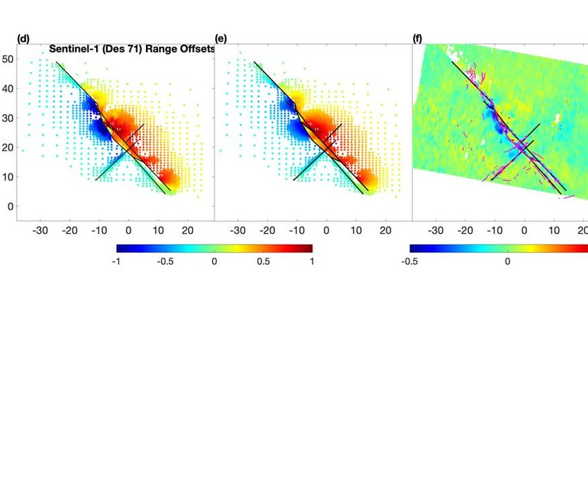
the mainshock. Analysis of the near-field GNSS data indicated that post-seismic
displacements did not exceed a few tens of millimeters in the months following the
earthquakes (Floyd et al., 2020) and are therefore negligible compared to the coseismic
displacements. The pre-seismic scenes were chosen to minimize the time span and
perpendicular baselines of the coseismic pairs. The resulting data set is summarized
in Table 1.
 All interferometric pairs were processed using GMTSAR (Sandwell et al., 2011).
The topography contribution to the radar phase was calculated and removed using
digital elevation data from the Shuttle Radar Topography Mission (SRTM) with 30 m
resolution (Farr and Kobrick, 2000). The images were co-registered using a geometric
alignment. Even in case of a perfect alignment, meter-scale surface displacements near
the earthquake rupture introduce phase discontinuities across the burst boundaries in
Sentinel-1 interferograms. Because the observed phase discontinuities across the burst
boundaries are small, here we simply neglect them. In general, such discontinuities
can be removed using a coseismic model to compute a range- and azimuth-dependent
alignment, similar to corrections for the ionospheric perturbations (e.g., Wang et al.,
2017).
 To avoid artifacts due to unwrapping errors in the near field of the earthquake
ruptures (where the decorrelation noise can be large), we unwrapped the radar phase
using a conservative branch-cut algorithm (Goldstein et al., 1988). The resulting
line of sight (LOS) displacements are shown in Figures 2a-d. To quantify surface
displacements in the near field of the earthquake ruptures where the radar phase
cannot be confidently unwrapped due to decorrelation, we computed range offsets
using Sentinel-1 data (Figure 2e-f), and azimuth offsets using Cosmo-Skymed data
(Figure 2g-h). While the offsets are less accurate compared to the differential radar
phase, they are useful for locating the rupture and constraining the distribution of
slip in the shallow crust. Because the azimuth pixel size for Sentinel-1 TOPS mode is
almost an order of magnitude larger than the range pixel size, the Sentinel-1 azimuth
offsets have a low signal to noise ratio (SNR), and are not used for slip inversions. We
performed a quality check on all of the scenes used in the inversions, and manually
masked out a few areas that were strongly affected by local errors or noise.

GNSS data
The Ridgecrest earthquakes occurred in an area spanned by the Plate Boundary Ob-
servatory, a mature network of continuously recording GNSS sites. This gave rise to a
large set of well-constrained vector coseismic displacements. However, because the av-
erage spacing between continuous GNSS (cGNSS) sites of PBO is on the order of 10-20
km, the cGNSS data primarily constrain integral characteristics of seismic sources such
as the moment tensor and/or the scalar moment. In order to densify the GNSS cov-
erage in the near field, teams from the University of California San Diego, University
of California at Riverside, University of Nevada at Reno, and the US Geological Sur-
vey coordinated a post-event response to occupy existing geodetic benchmarks within
∼ 50 km from the earthquake rupture. Most of the selected benchmarks have been
surveyed multiple times over the last 30 years, and some were surveyed as recently
as several months prior to the July 2019 earthquakes (Floyd et al., 2020). We have
collected post-event data from 7 campaign sites: 0806, INYO, GS11, GS17, GS20,
GS22, and GS48. Some of the surveyed sites had benchmarks consisting of metal rods

 4

driven or cemented into the ground, with center markings, that required a tripod setup
(Figure 3a). At other sites, benchmarks consisted of a threaded pin encastered in a
concrete block. For such sites, a GNSS antenna can be attached directly to a pin,
without the need for a tripod (Figure 3b).
 The data were collected at 15 second sampling intervals, and RINEX files were
archived at UNAVCO (Fialko et al., 2019b). Following the post-event deployment, we
left the sites running to document the early post-seismic deformation transient (Fialko
et al., 2019a). Solutions for coseismic displacements derived from the campaign GNSS
measurements were presented in Floyd et al. (2020). We use the coseismic offsets
derived from campaign as well as continuous GNSS data (Floyd et al., 2020) along
with data described in sub-section “SAR data” in joint inversions for the static slip
models, as described in the next section.

Joint inversions of surface displacement data
In order to prepare the InSAR data for inversions for the sub-surface slip distribution,
we de-trended the interferograms using low-resolution inverse models. A wide-swath
capability of Sentinel-1 and ALOS-2 ensures that coseismic interferograms extend into
areas where coseismic displacements are negligible (Figure 1). The satellite orbits are
known sufficiently well such that the orbital errors should not introduce significant
long-wavelength trends in the data. However, we find that the long-wavelength trends
are often present, possibly due to propagation effects (e.g., regional variations in the
troposphere and/or ionosphere) and need to be accounted for. Even in the absence of
the long-wavelength artifacts, one needs to estimate the phase ambiguity corresponding
to the far-field (“zero”) displacements. We do so by performing inversions for the slip
distribution and the best-fitting linear (or, in case of ALOS-2, higher order) ramps in
the radar phase using coarsely discretized fault models and coseismic interferograms
(e.g., Fialko, 2004). In these preliminary inversions we limited the fault depth to
15 km, based on the depth distribution of seismicity (e.g., Ross et al., 2019) to avoid
trade-offs between spurious deep slip and the ramp coefficients, and assigned relatively
heavy weights to the cGNSS data. The best-fit ramps were subtracted from the radar
interferograms. Because the range offsets represent the same projection of the surface
displacement field as the radar interferograms, we de-trended the range offsets by
fitting a linear ramp to the residual between the detrended radar interferograms and
the offsets, for each of the satellite tracks. The estimated ramps were subtracted from
the range offsets, so that the latter have the same asymptotic behavior in the far
field as the detrended interferograms and the cGNSS data. The azimuth offsets from
Cosmo-Skymed were not included in the initial inversions because of a narrow swath
that may not extend into a region of vanishing coseismic displacements (Figure 1).
De-trending of the azimuth offsets was performed at the next stage using a refined slip
model. The azimuth offsets thus provide independent constraints only on the shallow
(depth < 5 km) part of the slip model, as intended.
 The de-trended interferograms and range and azimuth offset maps were sub-sampled
using a quad-tree algorithm (Jonsson et al., 2002; Simons et al., 2002). To avoid
oversampling in areas affected by high-frequency noise (atmospheric contributions,
unwrapping errors, phase decorrelation, etc.), we down-sampled the data iteratively
using model predictions (Wang and Fialko, 2015). Following an initial inversion in

 5

which the best-fit slip model was obtained, the location of the data samples was de-
termined by executing the gradient-based quad-tree algorithm on a model prediction.
The obtained resolution cells were populated by the mean values of data from the orig-
inal de-trended interferograms. Usually, two or three iterations are sufficient to achieve
a convergent set of data points. In order to capture the details of slip distribution near
the Earth’s surface, we more densely sampled the offsets data around the fault traces.
In particular, given the patch size of ∼ 1 km at the shallowest part of the slip model,
we sampled the near-field data starting with the minimum resolution cell of ∼ 250
m. The (spatially variable) unit look vectors for all data samples were computed by
averaging the original values in the same resolution cells as used for sub-sampling the
displacement data.
 The sub-surface fault geometry is typically not well known, and is usually either as-
sumed or estimated as part of a non-linear inversion of surface displacement data (e.g.,
Fialko, 2004; Simons et al., 2002). However, in case of the Ridgecrest earthquakes,
data from a dense seismic network and advanced processing algorithms provided a
catalog of accurately located aftershocks (e.g., Ross et al., 2019) that can be used to
infer the rupture geometry throughout the seismogenic zone, under the assumption
that aftershocks are illuminating the ruptured faults and/or their immediate neigh-
borhood. We approximate the ruptures that produced the M6.4 foreshock and the
M7.1 mainshock by a set of rectangular fault segments that honor multiple available
data sets, including the aftershock locations (Ross et al., 2019), geologically mapped
fault traces (Ponti et al., 2020), and surface offsets from the space geodetic imaging
(Figure 2). The inferred geometry is illustrated in Figure 4 (also, see Supplemental
Figures S3-S4).
 Notable features of the aftershock distribution are: (i) change in the dip angle
around the epicenter of the M7.1 event, with a steep SW dip in the northern part of the
rupture, and a NE dip in the southern part; (ii) two sub-parallel NW-trending strands
of seismicity in the southern section; (iii) clear offsets between the surface rupture trace
and the projection of the aftershock cloud toward the surface in the central part of the
rupture (shown by the dotted and solid black lines, respectively, in Figure 4a). We
interpret this offset as a shallow splay structure that connects the surface rupture to the
main fault strand at depth that is expressed in the aftershock activity (Figure 4b). The
shallow dipping splay fault is not expressed in microseismicity, as is the “main” rupture
in the shallow crust, presumably because of the velocity-strengthening conditions at
low temperature and normal stress (e.g., Barbot et al., 2009a; Marone and Scholz,
1988; Mitchell et al., 2016; Rice and Tse, 1986). As we show below, the shallow
splay structure has nevertheless produced a large coseismic offset. The data shown
in Figure 4 also suggest that except for numerous cross-faults, the NW-striking fault
at depth is quite linear and exhibits less variability in strike compared to the surface
expression of the earthquake rupture.
 We extended the rectangular segments approximating the fault geometry to the
depth of 25 km, and by several km beyond the mapped fault traces along-strike, and
sub-divided each segment into slip patches which sizes gradually increase from about
1 km (along-strike and down-dip) at the top of the fault to about 5-10km at the
bottom, following a geometric progression to ensure that the model resolution does
not decrease with depth (Fialko, 2004). We computed Green’s functions for the strike
and dip components of slip on each patch for every observation point. As there are
many more data points than the degrees of freedom, the system is over-determined

 6

and is solved by minimizing the L2 norm of the residual. We applied a positivity
constraint on strike-slip components, such that no slip on the NE-trending segments
was allowed to be right-lateral, and no slip on the NW-trending segments was allowed
to be left-lateral. No positivity constraints were imposed on the dip-slip components,
but the latter were more strongly smoothed compared to the strike-slip components
to avoid spatially oscillating slip patterns. The first-order Tikhonov regularization
(e.g., Golub et al., 1999) was applied to avoid extreme variations in slip between the
adjacent fault patches. This also refers to complex intersections between different fault
segments (e.g., between the shallow splay faults and the main fault), in which case the
“neighboring” patches were identified based on a distance between the patch edges.
 We further regularized the problem by imposing “soft” zero-slip boundary condi-
tions (wS=0, where S is an unknown slip magnitude, and w is a prescribed weight) at
the fault edges, except for most of the edges at the free surface that were left uncon-
strained. While the solution does not exhibit artifacts without a zero-slip boundary
condition (e.g., no spurious large slip at the distant edges of the fault model), the latter
helps ensure a well-behaved asymptotic decay of slip away from the source region. We
also applied a soft zero-slip boundary condition at some segments of the fault trace
at the surface where the data do not show a displacement discontinuity (e.g., on the
eastern branch of the M7.1 rupture just south of the epicenter). This helps prevent a
spurious shallow slip due to smoothness constraints on the slip distribution and rela-
tively sparse sub-sampled points, as the displacement gradients across a “blind” fault
trace may be relatively small (e.g., Wang and Fialko, 2015). The optimal values of
the smoothness parameters and the relative weighting of different data sets (Sentinel-
1, ALOS-2, Cosmo-Skymed, continuous and campaign GNSS) used in the inversion
were determined using the Chi-Squared statistics (see figure S1 in the Supplemental
Materials). We point out that while the regularization using smoothness constraints
may appear as a somewhat arbitrary mathematical cure to the ill-conditioned nature
of inverse problems, it does serve a purpose of discriminating against solutions that
violate physical constraints such as the finite fault strength. Under a typical set of as-
sumptions about the data and the model parameters, a Tikhonov-type regularization
yields results that are similar to those obtained using the Bayesian inference methods
that are however much more computationally expensive (e.g., Bishop, 1995; Vogel,
2002).
 We performed two sets of inversions, one using Green’s functions for a homogeneous
elastic halfspace (Okada, 1985), and another for a layered elastic halfspace (Wang et al.,
2003). For the latter, we computed elastic moduli from the three-dimensional (3-D)
seismic tomography models of the Ridgecrest area (Hauksson and Unruh, 2007; Zhang
and Lin, 2014). While the data in principle allow one to compute Green’s functions
for an elastic halfspace with a 3-D distribution of elastic moduli (e.g., Barbot et al.,
2009b), the predicted deformation due to fault slip is mostly sensitive to variations in
the elastic moduli with depth, as variations in the lateral direction are relatively minor.
The average 1-D elastic rigidity structure used in our models is shown in Figure 5. For
the sake of consistency, we adopted the same fault geometry in the homogeneous and
layered halfspace models. In case of the layered models, rectangular fault patches were
approximated by a superposition of point sources.
 In addition to solving for the slip distribution given the assumed fault geometry,
we performed inversions using a grid search in which the dip angles of various fault
segments were allowed to vary. Results of these inversions are presented in the Supple-

 7

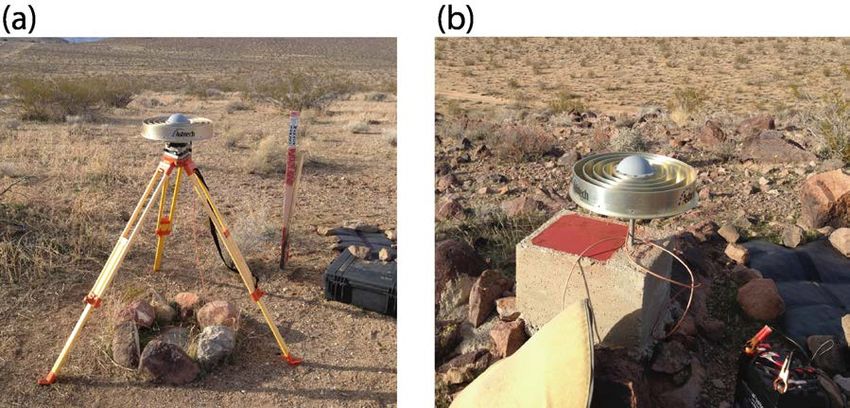
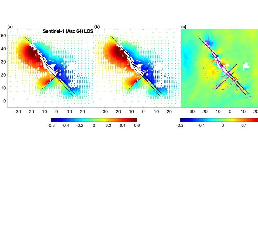
mental Materials (Figures S2, S5), and in general lend support to the fault geometry
constrained by the aftershock data (Figure 4).

Best-fit models: Results
Figure 6 shows the sub-sampled data points, predictions of the best-fit models, and
residuals (the difference between the data and the model predictions) for the Sentinel-1
interferograms from the ascending and descending tracks. We compute residuals at
the original (unsampled) resolution to illustrate the model fit to all of the data points,
including those that were not used in the inversion. Overall, the model fits the main
features of the displacement field quite well, with the variance reduction of more than
94%. Most of the misfit is concentrated near the rupture trace, where the assumption
of elastic deformation off of the fault plane is likely violated (e.g., Kaneko and Fialko,
2011). Figure 7 shows the model fit to the Sentinel-1 range offsets. Model fits to the
ALOS-2 and Cosmo-Skymed data are presented in Supplemental Materials (figures S6-
S7). A comparison with other proposed models of the Ridgecrest earthquakes shows
that our model is able to explain the data reasonably well (Wang et al., 2020).
 Figure 8 shows the observed and modeled horizontal displacements at the contin-
uous and campaign GNSS sites. We find that models that provide a good fit to the
SAR data (provided the latter are available from a diverse set of look angles) are able
to accurately “postdict” the independent GNSS data. The GNSS data therefore do
not need to be heavily weighted in the joint inversions. The GNSS data are however
quite useful for estimating and removing the long-wavelength trends and the “zero
displacement” uncertainty in the LOS displacements, as discussed in section “SAR
data”. As one can see in Figure 8, our best-fit model renders a good agreement with
the GNSS data, particularly in case of cGNSS (Figure 8a). For the campaign data,
the fit is also adequate for sites that experienced large coseismic displacements. Sites
with small displacements (and thus reduced SNR) render a poorer fit, in particular
because many of the sites had the most recent occupation 15-20 years ago, so there is
a large uncertainty in extrapolating the pre-seismic velocity (Floyd et al., 2020). Cyan
triangles in Figure 8b denote campaign sites at which data were collected shortly after
the July 2019 events, but not included in the inversion. In particular, we excluded
sites at which the angle between the observed and modeled horizontal displacements
exceeded 45◦ (GS04, GS25), or the magnitude of the observed and modeled horizontal
displacements differed by more than a factor of two (GS16). For site GS20, no coseis-
mic solution is available as the early post-earthquake data were corrupted because of
a receiver malfunction.
 Figures 9 and 10 show the slip distribution for the best-fit models assuming the
homogeneous and layered elastic half-space, respectively. As expected, the slip distri-
butions look similar; the main difference is that the slip is somewhat shallower and on
average smaller in case of a homogeneous half-space compared to a layered half-space
(e.g., Fialko, 2004). Tests using synthetic data indicate that the model resolution is
not strongly dependent on depth (see Supplemental Figure S9).
 We evaluate the “geodetic” moment magnitude Mg = 2/3(log10 GP − 9.1), where
G = 33 GPa is the nominal shear modulus, and P is the seismic potency, computed as
an algebraic sum ΣN i=1 Ai Si , where N is the number of slip patches (dislocations), and
Ai and Si are the area of, and the amplitude of slip on, patch i. Our models (Figures 9

 8

and 10) correspond to a composite event consisting of the foreshock and the mainshock.
Assuming that the foreshock was dominated by slip on the left-lateral faults 6 and 7,
and the mainshock was dominated by slip on the right-lateral faults 1-5 (see Figure 4
for the segment numbers), we estimate Mg of 6.42 for the foreshock, and 7.03 for the
mainshock in case of the homogeneous half-space model. In case of the layered half-
space model, the respective values of the geodetic moment magnitude are 6.46, and
7.10. Thus the geodetic moments inferred from inversions of static displacements are
in a good agreement with the seismic moments derived from the waveform spectra
(see Data and Resources Section in the Supplemental Materials). This is similar to
findings from previous studies of large events for which high-quality data are available
(e.g., Barbot et al., 2009a; 2008b; Fialko, 2004; Fialko et al., 2005b; Simons et al.,
2002; Wang and Fialko, 2018). In addition to providing a better agreement with the
seismic data, more complex (and presumably more realistic) layered models appear to
be more consistent with certain features of the geodetic data. While the homogeneous
and layered half-space models on average fit the geodetic data equally well, we find
that the layered models do a better job fitting the far-field decay of the coseismic
displacements (Figure S8).
 Apart from cross-faults that persist throughout the seismogenic layer (Ross et al.,
2019), the M7.1 rupture appears to be geometrically simpler at depth than near the
surface, where it branches out into splay faults of variable dip and strike. Accurately
located aftershocks indicate a fairly linear rupture that strikes ∼ 320◦ (Figure 4a),
with a gentle “helix-like” rotation from the westward dip in the north, to the eastward
dip in the south (Figure 4b). In contrast, geodetically and geologically mapped fault
trace exhibits deviations from the main trend illuminated by aftershocks, both along
strike and down dip. In particular, the fault trace is shifted to the west with respect to
the aftershock cloud in the central part of the rupture (Figure 4a), where the largest
slip is inferred from the inversion (Figures 9 and 10). The shift is larger than that
estimated by projecting the steeply dipping aftershock lineations to the surface. We
interpret these observations as indicating a “Y-shaped” rupture geometry in the top
few kilometers of the crust (Figure 4b), such that the main fault strand splits into
two (or more) splay faults with variable dip angles above the depth of 3-4 km. A
similar structure is also present to the north of the epicenter, where the two conjugate
faults dipping toward each other form a mini-graben, with subsidence in between
the faults, (see Figure 7a, around (-15,35) km in local coordinates), which requires a
dip-slip component on the shallow splay faults (Figures 9 and 10). We refer to this
preferred model as “Model A”. We point out that the rather detailed inferences about
the sub-surface fault geometry result from a joint analysis of precise seismic, geodetic,
and geologic data, and would not be possible from consideration of individual data
sets. For example, the aftershock data alone would be insufficient to reveal the details
of the rupture geometry in the uppermost crust which is largely aseismic, and the
geodetic and geologic data alone would be insufficient to detect changes in the fault
dip angle with depth (Figure 4). For the sake of completeness, we also considered an
alternative fault geometry in which the central part of the earthquake rupture consists
of two sub-parallel sub-vertical non-intersecting faults. The respective model (Model
B) is presented in the Supplementary Materials (Figures S10 and S11). While a sub-
vertical western branch results in a somewhat better fit to the data on the western side
of the fault, it would imply that the respective rupture segment is essentially devoid
of aftershocks throughout the seismogenic layer, which we deem unlikely.

 9

Stress changes due to the M6.4 foreshock and pos-
sible triggering of the M7.1 mainshock
A close spatiotemporal correlation between the M6.4 foreshock and the mainshock
is suggestive of a cause and effect relationship, and raises a question about possible
triggering mechanisms. A number of models were considered to explain interaction
between earthquakes, including static (Anderson and Johnson, 1999; Caskey and Wes-
nousky, 1997; Hardebeck et al., 1998; King et al., 1994; Ziv and Rubin, 2000) and
quasi-static (Deng and Sykes, 1997; Jonsson et al., 2003; Pollitz and Sacks, 2002;
Segall, 1989) stress transfer, triggering by dynamic stress changes (Bellardinelli et al.,
1999; Felzer et al., 2002; Gomberg et al., 1997; Lomnitz, 1996; Tymofyeyeva et al.,
2019), etc. The 2019 Ridgecrest sequence offers a great opportunity to test the pro-
posed models, not only because it was exceptionally well recorded, but also because it
has a history of perturbations by nearby seismic events, in which only the most recent
perturbation(s) of July 2019 culminated in a major earthquake.
 While our finite fault model corresponds to a combination of the M6.4 foreshock and
the mainshock, a good agreement between the geodetic moments computed for the left-
and right-lateral faults, on the one hand, with the seismic moments of the foreshock
and the mainshock, on the other hand, suggests that the seismic moment release due
to the M6.4 foreshock was dominated by slip on the left-lateral NE-striking faults
(segments 6 and 7 in Figure 4a). This in turn suggests that the foreshock involved
relatively minor coseismic slip on a right-lateral NW-trending fault revealed by the
aftershock activity following the M6.4 event (Chen et al., 2020; Ross et al., 2019). We
verify this inference by comparing surface displacements due to the left-lateral faults
from our best-fitting slip model to the GNSS observations of coseismic offsets due to
the M6.4 event (Floyd et al., 2020). Figure S12 shows the model predictions (red
arrows) and the observed horizontal displacements (blue arrows) from the continuous
(white dots) and campaign (yellow triangles) GNSS sites. The data and the model
predictions are in general agreement, including the high-fidelity cGNSS data. The fit
to the campaign GNSS data is surprisingly good, considering that some of the sites
have not been surveyed up to ∼ 20 years prior to the 2019 earthquakes. While these
results confirm that the moment release due to the M6.4 foreshock was dominated
by slip on the left-lateral faults (approximated by segments 6 and 7 in our coseismic
model, see Figure 4a), below we show that some amount of slip on the right-lateral
NW-striking rupture is required to produce positive static Coulomb stress changes at
the hypocenter of the M7.1 mainshock.
 We ran several tests to see how much slip could have occurred on a right-lateral
fault during the M6.4 foreshock. The model starts to notably over-predict the GNSS
data if the magnitude of an equivalent event on a right-lateral fault exceeds 5.8 (which
corresponds to ∼ 0.4 m of average slip on a a NW-striking fault segment). Figure 11
shows the observed and modeled horizontal displacements due to the M6.4 foreshock
involving slip on a system of high-angle antithetic strike-slip faults (denoted by green
lines in Figure 11). We note that M5.8 is an upper bound on the equivalent amount
of slip on the right-lateral fault. A larger moment release on the respective rupture
segment would result in an over-prediction of both the surface displacements measured
by the GNSS, and the scalar seismic moment (M6.4, see Data and Resources).
 We used finite fault models derived for the M6.4 event to compute static stress
changes at the hypocenter of the M7.1 mainshock. An important parameter in es-
 10

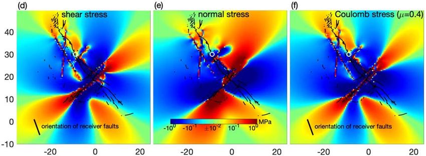
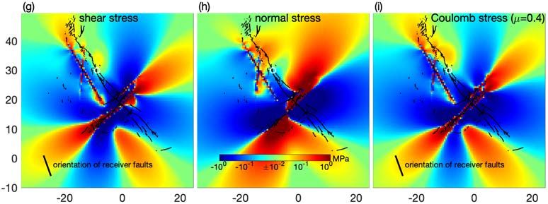
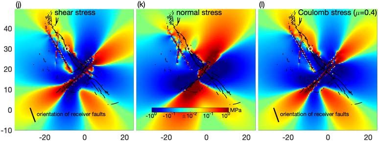
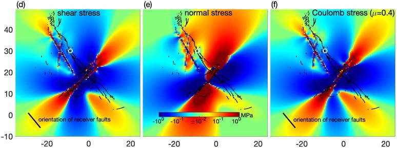
timation of the induced stress changes is the orientation of a receiver fault. This is
particularly relevant for the M7.1 Ridgecrest event given its complicated rupture ge-
ometry. In previous studies (e.g., Barnhart et al., 2019) static stress changes at the
hypocenter of the July 5 mainshock were computed assuming that the earthquake
rupture at depth follows the strike of the fault trace at the Earth surface. However,
a comparison of the geometry of precisely relocated aftershocks and the fault trace
show that the two are not necessarily correlated, as discussed in the previous section.
Therefore we performed calculations for a range of possible fault orientations (see Data
and Resources). Unless noted otherwise, all stress calculations presented below were
performed using layered elastic half-space models assuming a rigidity structure shown
in Figure 5. Figures 12a-c show stress perturbations due to slip on the left-lateral
fault segments 6 and 7 (see Figures 4 and 11) resolved on vertical planes striking
320◦ , coincident with the overall trend of aftershocks of the M7.1 rupture (Figures 4).
Stresses were computed at the hypocenter depth of the M7.1 event. Estimates of the
hypocenter depth vary between 2 and 8 km below the mean sea level, depending on a
method used (Hauksson and Jones, 2020). In our calculations we assume the depth of
7 km, accounting for the local elevation, and close to the values suggested by the full
waveform inversions, as most reliable (Hauksson and Jones, 2020). Numerical tests
show that the computed stress changes are not strongly dependent on the assumed
depth of the hypocenter of the M7.1 event.
 As one can see from Figures 12a-c, both shear and normal stress changes caused
by slip on the left-lateral faults involved in the M6.4 foreshock at the hypocenter of
the M7.1 rupture are close to zero, assuming that the mainshock nucleated on a slip
plane aligned with the general trend of the M7.1 rupture (Figures 4). The computed
Coulomb stress change is negligible compared to the negative Coulomb stress change
due to a pair of M5+ earthquakes that occurred in 1995 (Hauksson et al., 1995) in the
immediate vicinity of the hypocenter of the 2019 M7.1 event (Figure 12d-f, also see
Figures S15 and S16 in the Supplemental Materials). A more northerly fault strike of
340◦ , consistent with a focal mechanism derived from the P-wave arrivals (see Data
and Resources Section), provides for a more favorable orientation (Figure 12i), but
the resolved Coulomb stress is still negative or close to zero. These calculations show
that slip on the left-lateral faults that dominated the moment release from the M6.4
foreshock had a nearly neutral effect on the nucleation of the mainshock, and was
certainly insufficient to overcome the stress shadow cast by the 1995 events. Allowing
for a right-lateral slip on the NW-striking fault with an equivalent moment magnitude
of 5.8 results in the positive Coulomb stress changes at the mainshock hypocenter
(Figure 12l). Our calculations indicate that if the M7.1 event was triggered by static
stress transfer due to foreshocks, the triggering was due to slip on the same right-lateral
fault that was subsequently ruptured by the mainshock.
 We also investigated the role of the second largest foreshock, the M5.4 event that
occurred just hours before, and a few kilometers away from the hypocenter of the
mainshock. An earlier study by Barnhart et al. (2019) assumed that the M5.4 event
occurred on a NW-trending right-lateral fault, and estimated a positive Coulomb stress
change of ∼ 70 kPa at the hypocenter of the M7.1 event. However, detailed seismic
studies showed that the M5.4 aftershock occurred on a left-lateral NE-trending fault
(e.g., Shelly, 2020). Given a relatively small size of the foreshock, we generated a fi-
nite fault model assuming a circular rupture with a Gaussian slip distribution, subject
to a constraint that the geodetic moment equals the seismic moment. The rupture

 11

centroid and the effective radius were chosen such that most of the precisely located
aftershocks of the M5.4 event occur on a periphery of the assumed slip distribution,
as expected from the stress concentration arguments (e.g., Fialko, 2015). The calcu-
lated Coulomb stress changes at the mainshock hypocenter were found to be negative.
However, sensitivity tests showed that the results are quite dependent on the assumed
position of the centroid of the M5.4 rupture, because of its close proximity to the
mainshock hypocenter. In particular, perturbing the along-strike centroid location by
2 km (likely within the uncertainties of the assumed slip distribution) affects the sign
of the cumulative Coulomb stress change due to the 1995-2019 pre-mainshock sequence
(Figure 13). Thus the answer to the question “was the nucleation of the M7.1 main-
shock advanced by the cumulative static stress changes due to the nearby earthquakes”
depends on details of slip models of the respective earthquakes, most notably the 2019
M5.4 foreshock, that are not well constrained by the available data. For values of the
effective coefficient of friction that are higher than that assumed in calculations pre-
sented in this study (0.4), the predicted Coulomb stress changes are more negative, as
the normal stress changes at the mainshock hypocenter are predominantly compressive
(Figure 13b,e).
 It is interesting to note that the hypocenter of the 2019 M7.1 event has experienced
positive Coulomb stress changes due to shaking from the nearby events that were con-
siderably (up to an order of magnitude) higher than the estimated static stress changes
(see Figure S17 in the Supplemental Materials), yet the former failed to trigger a major
earthquake at the time of shaking. This is evidence for the importance of quasi-static
nucleation, rather than a critical yield stress, as the condition for triggering. Based
on the results presented in this section, we conclude that the 2019 M7.1 mainshock
nucleated on a fault oriented 340◦ (20 degrees west of north) that was likely nudged
toward failure by the M6.4 foreshock, and subsequently either encouraged or discour-
aged by the M5.4 foreshock. Upon nucleating, the rupture propagated along a system
of pre-existing faults on average striking 320◦ (40 degrees west of north). Activation
of the pre-existing faults that were presumably less optimally oriented for failure with
respect to the local stress field compared to the nucleation site could result from the
onset of dynamic weakening (e.g., Brown and Fialko, 2012; Di Toro et al., 2011; Reches
and Lockner, 2010; Rice, 2006).

Discussion
The 2019 M7.1 Ridgecrest earthquake shares a lot of similarities with the previous
major earthquake that occurred in the Eastern California Shear Zone, the 1999 Hector
Mine event (Figure 14). Both events nucleated on a fault strand striking at a larger
angle compared to the average strike of the whole rupture. In case of the Hector
Mine event, the fault strike correlates with topography (Fialko et al., 2005a); however,
no such correlation exists in case of the Ridgecrest event, so that stresses due to
topography cannot explain different orientations of the nucleation sites. A more likely
explanation is that both earthquakes nucleated on a local structure that was more
favorably oriented with respect to the regional stress field, and proceeded to rupture
pre-existing faults that have been rotated away from an optimal orientation over time
(e.g., by simple shear). If so, the rupture process may have involved dynamic triggering
and weakening of the pre-existing faults.

 12

Both the Ridgecrest and the Hector Mine ruptures exemplify complexity of imma-
ture developing strike-slip fault zones, with multiple sub-parallel branches and along-
strike variations in the dip angle. Coseismic slip on closely spaced sub-parallel fault
strands is puzzling, as dynamic rupture on a given fault interface is expected to dis-
courage slip on nearby potential slip interfaces. More sophisticated dynamic rupture
models are needed to better understand observations of slip on multiple sub-parallel
fault strands. Finally, for both the Ridgecrest and the Hector Mine events, some of
the fault strands broke the surface, while other strands remained blind and could only
be detected with the help of precisely located aftershocks.
 Among the main differences between the two events are the abundant cross-faults
and shallow splay faults in case of the Ridgecrest earthquake. In part this difference
could be attributed to regional variations in the stress regime. The Ridgecrest earth-
quakes occurred in a transtensional domain with concurrent strike-slip and normal
faulting, as evidenced by e.g. the 1995 earthquake sequence that involved a pair of
closely spaced strike-slip and normal faults (Hauksson et al., 1995, also, see Supple-
mental Materials, Figures S13 and S14). The shallow splay faults inferred from our
inversions have dip angles around 60-70◦ , close to optimal orientation for normal faults.
We interpret them as normal faults activated to accommodate a combination of the
right-lateral slip and extension across the ECSZ. The geometry of our best-fit mod-
els in the shallow crust closely resembles the so-called “flower structures” recognized
on a number of strike-slip faults world-wide (Bayasgalan et al., 1999; Harding, 1985;
Sylvester, 1988).
 It is of interest to evaluate how the coseismic slip amplitude varies with depth.
Previous studies have suggested that for a number of M∼ 7 strike-slip earthquakes
the amount of slip in the middle of the seismogenic layer systematically exceeds the
amount of slip at the surface (Fialko et al., 2005b; Hussain et al., 2016; Wang et al.,
2014). While such behavior would be entirely expected for faults cutting through the
velocity-strengthening layer in the top few kilometers of the Earth’s crust (Hudnut
and Sieh, 1989; Johnson et al., 2006; Marone and Scholz, 1988), where the coseismic
slip is inhibited and most of slip occurs aseismically, for many faults that exhibit a
larger coseismic slip at depth there is no evidence that aseismic slip is present and/or
sufficiently robust to balance the slip budget. Such behavior, known as the shallow slip
deficit (SSD), could be attributed to a number of mechanisms, including the presence
of a soft damage zone (Barbot et al., 2008a), and dynamic damage due to propagating
rupture fronts (Kaneko and Fialko, 2011; Roten et al., 2017). Inversions of high-quality
geodetic data also show that a number of large strike-slip (or mixed mode) earthquakes
are not associated with the SSD, although such events tend to be on a high end of the
M7-M8 range (e.g., Tong et al., 2010; Zinke et al., 2014), possibly indicating differences
between rupture styles on mature and immature faults.
 Figure 15a shows a normalized distribution of slip as a function of depth for the
M7.1 Ridgecrest earthquake (black solid line) obtained from our best-fitting model for a
layered half-space (Figure 10), as well as for a number of other strike-slip earthquakes of
comparable size for which high-quality geodetic data are available (color dashed lines).
As one can see from Figure 15a, the maximum average slip due to the mainshock of
the Ridgecrest sequence occurred in the depth interval between 3-4 km, essentially the
same as inferred for other major strike-slip earthquakes analyzed using a consistent
methodology. The estimated amount of the SSD is on the order of 30%, although
the amplitude obviously depends on the degree of smoothing, with greater smoothing

 13

resulting in smaller variations in the slip amplitude with depth. It is interesting to
note that the inferred peak in the seismic moment release for system-size earthquakes
that rupture the entire seismogenic layer (Figure 15a) is also apparent in the depth
distribution of small earthquakes. Figure 15b shows the depth distribution of all of
seismicity in California, as well as the aftershocks of the 2019 Ridgecrest earthquakes
(see Data and Resources Section). We culled the earthquake catalogs to exclude events
that have an absolute depth error greater than 1 km, and assigned the data to 1 km
depth bins. The resulting data set consisting of ∼ 106 events has a maximum in
the mid-upper seismogenic zone, approximately in the same depth interval as the
peak in the coseismic moment release by large earthquakes (Figure 15a). This is in
contrast with models that predict that the most favorable conditions for the earthquake
occurrence are met at the bottom of the seismogenic zone (Jiang and Fialko, 2016;
Jiang and Lapusta, 2016; Sibson, 1982). Given the average thickness of the seismogenic
layer in the continental crust on the order of 12-14km (e.g., Wright et al., 2013), results
shown in Figure 15 suggest that the depth interval most conducive to unstable slip is
in the upper part of the seismogenic zone. Catalogs of precisely located earthquakes
with low magnitude of completeness from other seismically active regions are needed to
test whether a similar depth dependence of “seismogenic potential” exists elsewhere.

Conclusions
The M7.1 July 5 2019 Ridgecrest earthquake was the largest earthquake in southern
California since the 1999 Hector Mine earthquake, with which it shared a number of
similarities. The Ridgecrest earthquake is characterized by a complex rupture geom-
etry involving sub-parallel fault strands, along-strike variations in the dip angle, and
shallow variations in the fault strike. The maximum slip occurred on shallow splay
faults that were likely re-activated normal faults forming a classic “flower structure”
on top of a reasonably straight right-lateral strike-slip fault at depth. Nucleation of
unstable slip at the hypocenter of the M7.1 mainshock was discouraged by the pair of
the M5+ events that occurred in the immediate vicinity of the hypocenter in August-
September of 1995, only weakly if at all affected by slip on a left-lateral branch of the
M6.4 foreshock, encouraged by slip on a right-lateral branch of the M6.4 foreshock,
and likely discouraged by the M5.4 foreshock that occurred hours before the main-
shock. Static stress changes near the hypocenter resolved on a mean trend of the M7.1
rupture were less favorable for failure compared to stress changes resolved on a more
northerly striking fault plane indicated by the first motion data. This suggests that
the M7.1 mainshock may have been triggered by the M6.4 foreshock on a slip patch
that was optimally oriented for failure with respect to the local stress field, and sub-
sequently triggered unstable slip on a less favorably oriented pre-existing right-lateral
fault system. Dynamic stress changes from the nearby earthquakes failed to trigger the
mainshock, despite the fact that they were much larger than any static stress change
that might have advanced the nucleation of unstable slip. Slip models derived from
inversions of surface deformation data reveal a moderate amount of shallow slip deficit.
Subsequent studies of postseismic deformation will show if the inferred amount of the
co-seismic slip deficit can be accommodated by means of creep in the uppermost crust.
The estimated depth of the maximum slip averaged along the rupture length is 3-4
km, similar to results from previous studies of major strike-slip earthquakes, and to

 14

the depth distribution of precisely located seismicity in California, suggesting that the
respective depth interval maximizes a potential for seismic instabilities.

Acknowledgments
We thank the two anonymous reviewers and the Editor Timothy Dawson for thorough
and insightful reviews. This study was supported by NASA (grant 80NSSC18K0466)
and NSF (grants EAR-1841273 and RAPID 1945760). Sentinel-1 data were provided
by the European Space Agency (ESA) through Alaska Satellite Facility (ASF) and
UNAVCO. Digital Elevation data were provided by NASA and DLR. Some of the
figures were generated using the Generic Mapping Tools (GMT) (Wessel et al., 2013)
and Matlab.

 15

References
Ahmed, R., P. Siqueira, S. Hensley, B. Chapman, and K. Bergen (2011). A survey
 of temporal decorrelation from spaceborne L-Band repeat-pass InSAR, Remote
 Sensing of Environment, 115 2887–2896.

Anderson, G. and H. Johnson (1999). A new statistical test for static stress triggering:
 Application to the 1987 Superstition Hills earthquake sequence, J. Geophys. Res.,
 104 20153–20168.

Barbot, S., Y. Fialko, and Y. Bock (2009a). Postseismic deformation due to the Mw 6.0
 2004 Parkfield earthquake: Stress-driven creep on a fault with spatially variable
 rate-and-state friction parameters, J. Geophys. Res., 114 B07405.

Barbot, S., Y. Fialko, and D. Sandwell (2008a). Effect of a compliant fault zone
 on the inferred earthquake slip distribution, J. Geophys. Res., 113 B06404,
 doi:10.1029/2007JB005256.

Barbot, S., Y. Fialko, and D. Sandwell (2009b). Three-dimensional models of elasto-
 static deformation in heterogeneous media, with applications to the Eastern Cali-
 fornia Shear Zone, Geophys. J. Int., 179 500–520.

Barbot, S., Y. Hamiel, and Y. Fialko (2008b). Space geodetic investigation of the co-
 and post-seismic deformation due to the 2003 Mw 7.1 Altai earthquake: Implica-
 tions for the local lithospheric rheology, J. Geophys. Res., 113 B03403.

Barnhart, W. D., G. P. Hayes, and R. D. Gold (2019). The July 2019 Ridgecrest,
 California, earthquake sequence: Kinematics of slip and stressing in cross-fault
 ruptures, Geophys. Res. Lett., 46 11859–11867.

Bayasgalan, A., J. Jackson, J.-F. Ritz, and S. Carretier (1999). Forebergs’, flower
 structures, and the development of large intra-continental strike-slip faults: the
 Gurvan Bogd fault system in Mongolia, J. Struct. Geol., 21 1285–1302.

Bellardinelli, M. E., M. Cocco, O. Coutant, and F. Cotton (1999). Redistribution
 of dynamic stress during coseismic ruptures: Evidence for fault interaction and
 earthquake triggering, J. Geophys. Res., 104 14925–14945.

Bishop, C. M. (1995). Training with noise is equivalent to Tikhonov regularization,
 Neural computation, 7 108–116.

Brown, K. M. and Y. Fialko (2012). ”Melt welt” mechanism of extreme weakening of
 gabbro at seismic slip rates, Nature, 488 638–641.

Caskey, S. J. and S. G. Wesnousky (1997). Static stress change and earthquake trigger-
 ing during the 1954 Fairview Peak and Dixie Valley earthquakes, Central Nevada,
 Bull. Seism. Soc. Am., 87 521–527.

Chen, K., J.-P. Avouac, S. Aati, C. Milliner, F. Zheng, and C. Shi (2020). Cascading
 and pulse-like ruptures during the 2019 Ridgecrest earthquakes in the Eastern
 California Shear Zone, Nature Communications, 11 1–8.

 16

Deng, J. and L. R. Sykes (1997). Evolution of the stress field in Southern California
 and triggering of moderate-size earthquakes: A 200-year perspective, J. Geophys.
 Res., 102 9859–9886.
Di Toro, G., R. Han, T. Hirose, N. De Paola, S. Nielsen, K. Mizoguchi, F. Ferri,
 M. Cocco, and T. Shimamoto (2011). Fault lubrication during earthquakes, Nature,
 471 494–498.
Dokka, R. K. and C. J. Travis (1990). Role of the Eastern California shear zone in
 accommodating Pacific-North American plate motion, Geophys. Res. Lett., 17
 1323–1327.
Farr, T. and M. Kobrick (2000). Shuttle Radar Topography Mission produces a wealth
 of data, AGU Eos, 81 583–585.
Felzer, K. R., T. W. Becker, R. E. Abercrombie, G. Ekström, and J. R. Rice (2002).
 Triggering of the 1999 Mw 7.1 Hector Mine earthquake by aftershocks of the 1992
 Mw 7.3 Landers earthquake, J. Geophys. Res., 107 ESE–6.
Fialko, Y. (2004). Probing the mechanical properties of seismically active crust
 with space geodesy: Study of the co-seismic deformation due to the 1992
 Mw 7.3 Landers (southern California) earthquake, J. Geophys. Res., 109 B03307,
 10.1029/2003JB002756.
Fialko, Y. (2015), Fracture and Frictional Mechanics - Theory, In Schubert, G., editor,
 Treatise on Geophysics, 2nd. Ed., Vol. 4, pages 73–91. Elsevier Ltd., Oxford.
Fialko, Y., Z. Jin, E. Tymofyeyeva, and M. A. Floyd (2019a), Ridgecrest Califor-
 nia Earthquake Post-Event Response July 2019 UCSD, doi:10.7283/YJK0-B215,
 Technical report, UNAVCO, Inc., GPS/GNSS Observations Dataset.
Fialko, Y., Z. Jin, E. Tymofyeyeva, D. T. Sandwell, J. Haase, and M. A. Floyd (2019b),
 Ridgecrest California Earthquake Response July 2019 UCSD, doi:10.7283/N74Q-
 GA66, Technical report, UNAVCO, Inc., GPS/GNSS Observations Dataset.
Fialko, Y., L. Rivera, and H. Kanamori (2005a). Estimate of differential stress in the
 upper crust from variations in topography and strike along the San Andreas fault,
 Geophys. J. Int., 160 527–532.
Fialko, Y., D. Sandwell, M. Simons, and P. Rosen (2005b). Three-dimensional defor-
 mation caused by the Bam, Iran, earthquake and the origin of shallow slip deficit,
 Nature, 435 295–299.
Fialko, Y., M. Simons, and D. Agnew (2001). The complete (3-D) surface displacement
 field in the epicentral area of the 1999 Mw 7.1 Hector Mine earthquake, southern
 California, from space geodetic observations, Geophys. Res. Lett., 28 3063–3066.
Floyd, M., G. Funning, Y. A. Fialko, R. L. Terry, and T. Herring (2020). Survey and
 Continuous GNSS in the vicinity of the July 2019 Ridgecrest earthquakes, in press,
 Seismol. Res. Lett., 91.
Goldstein, R. M., H. A. Zebker, and C. L. Werner (1988). Satellite radar interferome-
 try: Two-dimensional phase unwrapping, Radio science, 23 713–720.
 17