Automatic load shedding scheme and the integration of new capacitors' controller in the South-West region of France to mitigate large scale ...
←
→
Page content transcription
If your browser does not render page correctly, please read the page content below
Automatic load shedding scheme and
    the integration of new capacitors’
controller in the South-West region of
France to mitigate large scale voltage
                             collapses

                         Geoffrey Senac

                             'HJUHHSURMHFWLQ
                          Electric Power Systems
                                   Second Level,
                         Stockholm, Sweden 2014

                            XR-EE-EPS 2014:010
SUPELEC & KTH
                              Double Degree
                           Electrical Engineering

              Master’s thesis report

Automatic load shedding scheme and the integration
of new capacitors’ controller in the South-West region
   of France to mitigate large scale voltage collapses

                           Geoffrey SENAC

       Supervisor at RTE                            Supervisors at KTH

     Hervé LEFEBVRE                             Lennart SÖDER
                                               Rujiroj LEELARUJI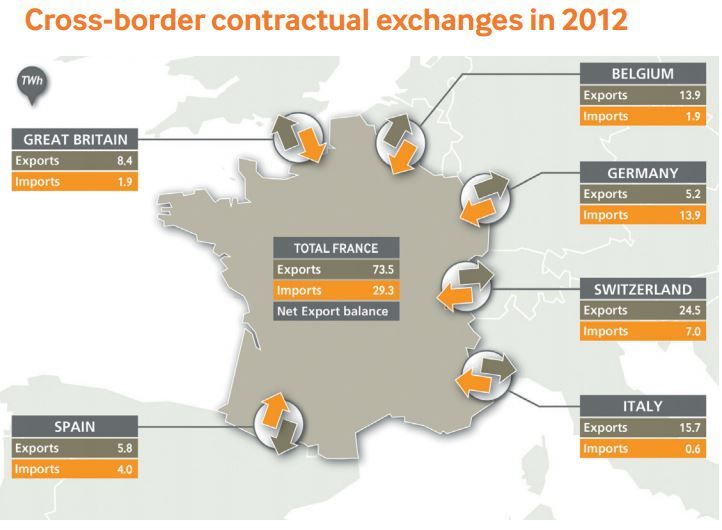
Master’s Thesis report page 1
Abstract

Since the modern world is totally dependent on electricity, it is necessary to ensure that elec-
trical power is generated and transmitted to end users with minimum interruptions. Given the
importance of electricity for the operation of our society, it is really important to fill continu-
ously good safety conditions. This policy must handle two major areas: reducing the risk of
occurrence of a crisis and its management if a very constraining disturbance happens. This
master’s thesis is mainly focused on this last point.

    With the continuous increasing of consumption and the high investment costs, it becomes
more complicated to ensure good safety margins, since the network is exploited closer to its
limits. A recent study demonstrates that the South-West region of France was prone to voltage
collapses after very severe faults and as a result the need of an under-voltage load shedding in
this region was evokated.

     In parallel, to ensure the voltage stability, RTE (Réseau de Transport d’Electricité - Elec-
tricity Transmission Network) has invested also in equipments such as capacitors and static
reactive power compensators. With newly installation of compensation means on the network,
the necessity to develop a new device called SMACC (Système avancé pour le contrôle de la
compensation - Advanced system for the control of the compensation) capable of handling more
efficiently the control of these batteries of capacitors has been highlighted.

    Ultimately the thesis focuses also on the new HVDC (High-voltage direct current) line
between France and Spain. This line is a key for long-term voltage stability study, since it
increases the exchange capacity between France and Spain, and has the ability to provide or
absorb reactive power to the network.
Acknowledgements

I would like to express my very great appreciation to my supervisor Hervé LEFEBVRE for
his welcome, patience guidance and continuous advice and for everything he taught me during
this master’s thesis regarding the system’s operation and more particulary the voltage stability
issues.

   I would also like to thank all the members of DES for their support and for integrating
me. I would like to give a special thank to Sebastien Murgey, Florent Xavier, Emilie Milin
and Philippe Juston for their help and the knowledge they shared with me on Convergence,
Eurostag and the transmission network.

    Then I would like to thank my KTH’s supervisors: Dr Luigi Vanfretti for validating the
choice of my Master’s thesis, Lennart Söder for being my final examiner and for his advice and
finally Dr Rujiroj Leelaruji for his continuous support, his advice and his patience all along the
thesis and for having read many times my thesis proposal as well as this report.

    Last but not least, I would like to dedicate this master’s thesis to my parents and to my
girlfriend Anissa. To my parents for the education, support and encouragement they provided
me over the years. They gave me much more that I could except, and without them I may
never have been the person I am today. To my girlfriend for her constant love, her patience
and support all along my studies even in the most difficult times.

   Finally I cannot conclude without having a huge thought to my brother and I wish him all
the best for the rest of his studies.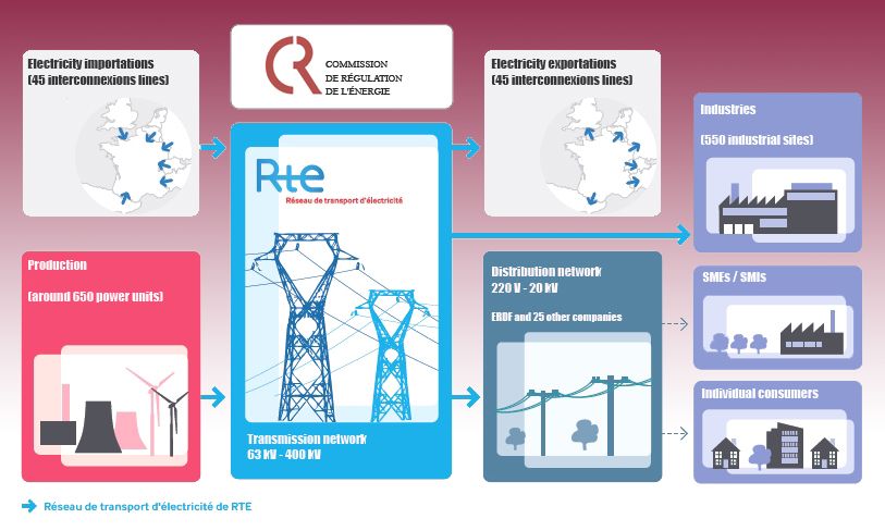
Contents

Abstract                                                                                                                                        2

Acknowledgements                                                                                                                                3

Table of Contents                                                                                                                              4

List of Figures                                                                                                                                 6

List of Tables                                                                                                                                  8

Abbreviations                                                                                                                                   9

1 Company                                                                                                                                      10
  1.1 Presentation of RTE . . . . . . . . . . . . .        .   .   .   .   .   .   .   .   .   .   .   .   .   .   .   .   .   .   .   .   .   10
      1.1.1 Historical background . . . . . . . .          .   .   .   .   .   .   .   .   .   .   .   .   .   .   .   .   .   .   .   .   .   10
      1.1.2 RTE group - public service missions            .   .   .   .   .   .   .   .   .   .   .   .   .   .   .   .   .   .   .   .   .   10
      1.1.3 Key figures . . . . . . . . . . . . . .        .   .   .   .   .   .   .   .   .   .   .   .   .   .   .   .   .   .   .   .   .   11
  1.2 The company organization . . . . . . . . . .         .   .   .   .   .   .   .   .   .   .   .   .   .   .   .   .   .   .   .   .   .   12
      1.2.1 On the French territory . . . . . . .          .   .   .   .   .   .   .   .   .   .   .   .   .   .   .   .   .   .   .   .   .   12
      1.2.2 Expertise and system department . .            .   .   .   .   .   .   .   .   .   .   .   .   .   .   .   .   .   .   .   .   .   13

2 Mission                                                                                                                                      15
  2.1 Current and upcoming challenges . . . .      .   .   .   .   .   .   .   .   .   .   .   .   .   .   .   .   .   .   .   .   .   .   .   15
      2.1.1 Supply-demand balance . . . . .        .   .   .   .   .   .   .   .   .   .   .   .   .   .   .   .   .   .   .   .   .   .   .   15
      2.1.2 Integration of Renewable Energy        .   .   .   .   .   .   .   .   .   .   .   .   .   .   .   .   .   .   .   .   .   .   .   15
      2.1.3 Electricity market’s development       .   .   .   .   .   .   .   .   .   .   .   .   .   .   .   .   .   .   .   .   .   .   .   16
  2.2 Master’s thesis objectives . . . . . . . .   .   .   .   .   .   .   .   .   .   .   .   .   .   .   .   .   .   .   .   .   .   .   .   17
      2.2.1 Aim of the project . . . . . . . .     .   .   .   .   .   .   .   .   .   .   .   .   .   .   .   .   .   .   .   .   .   .   .   17
      2.2.2 Thesis work outline . . . . . . .      .   .   .   .   .   .   .   .   .   .   .   .   .   .   .   .   .   .   .   .   .   .   .   17
      2.2.3 Outline . . . . . . . . . . . . . .    .   .   .   .   .   .   .   .   .   .   .   .   .   .   .   .   .   .   .   .   .   .   .   17

3 Theoretical study                                                                                                                            18
  3.1 Introduction of power system stability . . .         .   .   .   .   .   .   .   .   .   .   .   .   .   .   .   .   .   .   .   .   .   18
  3.2 Network model and performance . . . . . .            .   .   .   .   .   .   .   .   .   .   .   .   .   .   .   .   .   .   .   .   .   19
      3.2.1 Line model . . . . . . . . . . . . . .         .   .   .   .   .   .   .   .   .   .   .   .   .   .   .   .   .   .   .   .   .   19
      3.2.2 Maximal transmissible active power             .   .   .   .   .   .   .   .   .   .   .   .   .   .   .   .   .   .   .   .   .   22
      3.2.3 Reactive loss . . . . . . . . . . . . .        .   .   .   .   .   .   .   .   .   .   .   .   .   .   .   .   .   .   .   .   .   24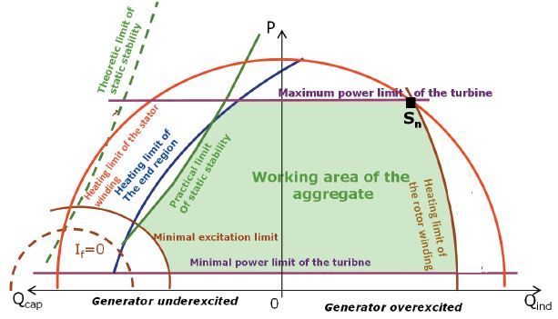
CONTENTS

         3.2.4 Influence of some parameters . . . . . . .             .   .   .   .   .   .   .   .   .   .   .   .   .   .   .   .   .   .   26
         3.2.5 Load modeling . . . . . . . . . . . . . . .            .   .   .   .   .   .   .   .   .   .   .   .   .   .   .   .   .   .   31
   3.3   Voltage control mechanisms . . . . . . . . . . . .           .   .   .   .   .   .   .   .   .   .   .   .   .   .   .   .   .   .   34
         3.3.1 Introduction . . . . . . . . . . . . . . . .           .   .   .   .   .   .   .   .   .   .   .   .   .   .   .   .   .   .   34
         3.3.2 Secondary Voltage Control . . . . . . . .              .   .   .   .   .   .   .   .   .   .   .   .   .   .   .   .   .   .   35
         3.3.3 On-load tap changers . . . . . . . . . . .             .   .   .   .   .   .   .   .   .   .   .   .   .   .   .   .   .   .   37
   3.4   Prevention of voltage instability . . . . . . . . . .        .   .   .   .   .   .   .   .   .   .   .   .   .   .   .   .   .   .   41
         3.4.1 Contingencies and margins . . . . . . . .              .   .   .   .   .   .   .   .   .   .   .   .   .   .   .   .   .   .   41
         3.4.2 Reliability degradation : Voltage Collapse             .   .   .   .   .   .   .   .   .   .   .   .   .   .   .   .   .   .   41
         3.4.3 Under Voltage Load Shedding . . . . . . .              .   .   .   .   .   .   .   .   .   .   .   .   .   .   .   .   .   .   42

4 Simulation tools                                                                                                                            45
  4.1 Convergence . . . . .     . . . . . . . . . . . . . .   .   .   .   .   .   .   .   .   .   .   .   .   .   .   .   .   .   .   .   .   45
      4.1.1 Convergence’s       static tool: HADES . .        .   .   .   .   .   .   .   .   .   .   .   .   .   .   .   .   .   .   .   .   45
      4.1.2 Convergence’s       dynamic tool: ASTRE           .   .   .   .   .   .   .   .   .   .   .   .   .   .   .   .   .   .   .   .   46
  4.2 Eurostag . . . . . . .    . . . . . . . . . . . . . .   .   .   .   .   .   .   .   .   .   .   .   .   .   .   .   .   .   .   .   .   47

5 Test of the SMACCs                                                                                                                          48
  5.1 Presentation of the SMACCs . . . . . . . .          .   .   .   .   .   .   .   .   .   .   .   .   .   .   .   .   .   .   .   .   .   48
      5.1.1 Context for this new control system           .   .   .   .   .   .   .   .   .   .   .   .   .   .   .   .   .   .   .   .   .   48
      5.1.2 Operating principle . . . . . . . . . .       .   .   .   .   .   .   .   .   .   .   .   .   .   .   .   .   .   .   .   .   .   51
      5.1.3 Challenges . . . . . . . . . . . . . .        .   .   .   .   .   .   .   .   .   .   .   .   .   .   .   .   .   .   .   .   .   52
  5.2 SMACCs study . . . . . . . . . . . . . . . .        .   .   .   .   .   .   .   .   .   .   .   .   .   .   .   .   .   .   .   .   .   52
      5.2.1 Preparatory work . . . . . . . . . . .        .   .   .   .   .   .   .   .   .   .   .   .   .   .   .   .   .   .   .   .   .   52
      5.2.2 Simulation on Convergence . . . . .           .   .   .   .   .   .   .   .   .   .   .   .   .   .   .   .   .   .   .   .   .   53
      5.2.3 Simulation on Eurostag . . . . . . .          .   .   .   .   .   .   .   .   .   .   .   .   .   .   .   .   .   .   .   .   .   55
  5.3 Conclusion . . . . . . . . . . . . . . . . . .      .   .   .   .   .   .   .   .   .   .   .   .   .   .   .   .   .   .   .   .   .   63

6 Setting up of an
  Under Voltage Load Shedding (UVLS)                                                                                                          64
  6.1 Context and Methodology . . . . . . . . . . . . .               .   .   .   .   .   .   .   .   .   .   .   .   .   .   .   .   .   .   64
  6.2 Voltage Stability study in South-West of France .               .   .   .   .   .   .   .   .   .   .   .   .   .   .   .   .   .   .   64
       6.2.1 Situation studied . . . . . . . . . . . . . .            .   .   .   .   .   .   .   .   .   .   .   .   .   .   .   .   .   .   64
       6.2.2 HVDC line . . . . . . . . . . . . . . . . .              .   .   .   .   .   .   .   .   .   .   .   .   .   .   .   .   .   .   65
       6.2.3 LSD model in Convergence and Eurostag                    .   .   .   .   .   .   .   .   .   .   .   .   .   .   .   .   .   .   66
       6.2.4 Simulations on Convergence . . . . . . . .               .   .   .   .   .   .   .   .   .   .   .   .   .   .   .   .   .   .   67
       6.2.5 Simulations on Eurostag . . . . . . . . . .              .   .   .   .   .   .   .   .   .   .   .   .   .   .   .   .   .   .   70
  6.3 Conclusion . . . . . . . . . . . . . . . . . . . . .            .   .   .   .   .   .   .   .   .   .   .   .   .   .   .   .   .   .   80

Bibliography                                                                                                                                  81

Master’s Thesis report                                                                                                                page 5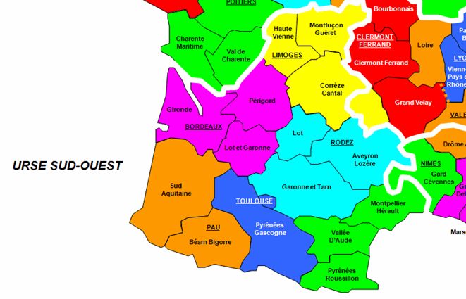
List of Figures

 1.1    Electrical System . . . . . . . . . . . . . . . . . . . . . . . . . . . . . . . . . . . . 11
 1.2    Cross border contractual exchanges in 2012 . . . . . . . . . . . . . . . . . . . . . 12
 1.3    Regional dispatching centers . . . . . . . . . . . . . . . . . . . . . . . . . . . . . . 13

 3.1    Per-phase equivalent circuit . . . . . . . . . . . . .     .   .   .   .   .   .   .   .   .   .   .   .   .   .   .   .   .   19
 3.2    Symplified model . . . . . . . . . . . . . . . . . . .     .   .   .   .   .   .   .   .   .   .   .   .   .   .   .   .   .   20
 3.3    Vector diagram . . . . . . . . . . . . . . . . . . . .     .   .   .   .   .   .   .   .   .   .   .   .   .   .   .   .   .   20
 3.4    Vector diagram . . . . . . . . . . . . . . . . . . . .     .   .   .   .   .   .   .   .   .   .   .   .   .   .   .   .   .   21
 3.5    Simple line model . . . . . . . . . . . . . . . . . . .    .   .   .   .   .   .   .   .   .   .   .   .   .   .   .   .   .   22
 3.6    Vector diagram . . . . . . . . . . . . . . . . . . . .     .   .   .   .   .   .   .   .   .   .   .   .   .   .   .   .   .   23
 3.7    Nose curve . . . . . . . . . . . . . . . . . . . . . .     .   .   .   .   .   .   .   .   .   .   .   .   .   .   .   .   .   23
 3.8    Nose curve : operating point . . . . . . . . . . . .       .   .   .   .   .   .   .   .   .   .   .   .   .   .   .   .   .   25
 3.9    Π Model . . . . . . . . . . . . . . . . . . . . . . . .    .   .   .   .   .   .   .   .   .   .   .   .   .   .   .   .   .   25
 3.10   Reactive loss . . . . . . . . . . . . . . . . . . . . .    .   .   .   .   .   .   .   .   .   .   .   .   .   .   .   .   .   26
 3.11   Impedance influence . . . . . . . . . . . . . . . . .      .   .   .   .   .   .   .   .   .   .   .   .   .   .   .   .   .   27
 3.12   Reactance influence . . . . . . . . . . . . . . . . . .    .   .   .   .   .   .   .   .   .   .   .   .   .   .   .   .   .   28
 3.13   Impedance influence . . . . . . . . . . . . . . . . .      .   .   .   .   .   .   .   .   .   .   .   .   .   .   .   .   .   29
 3.14   Generator equivalent circuit and phasor diagram .          .   .   .   .   .   .   .   .   .   .   .   .   .   .   .   .   .   29
 3.15   Generator operating limitations on a P-Q diagram           .   .   .   .   .   .   .   .   .   .   .   .   .   .   .   .   .   30
 3.16   Rotor current limitation . . . . . . . . . . . . . . .     .   .   .   .   .   .   .   .   .   .   .   .   .   .   .   .   .   31
 3.17   Loads classification . . . . . . . . . . . . . . . . . .   .   .   .   .   .   .   .   .   .   .   .   .   .   .   .   .   .   31
 3.18   Static load models . . . . . . . . . . . . . . . . . .     .   .   .   .   .   .   .   .   .   .   .   .   .   .   .   .   .   32
 3.19   Influence of the static load characteristics . . . . .     .   .   .   .   .   .   .   .   .   .   .   .   .   .   .   .   .   33
 3.20   Load response under voltage drop . . . . . . . . . .       .   .   .   .   .   .   .   .   .   .   .   .   .   .   .   .   .   34
 3.21   Secondary Voltage Control . . . . . . . . . . . . . .      .   .   .   .   .   .   .   .   .   .   .   .   .   .   .   .   .   36
 3.22   OLTC equivalent circuit . . . . . . . . . . . . . . .      .   .   .   .   .   .   .   .   .   .   .   .   .   .   .   .   .   38
 3.23   Nose curve . . . . . . . . . . . . . . . . . . . . . .     .   .   .   .   .   .   .   .   .   .   .   .   .   .   .   .   .   39
 3.24   Nose curve . . . . . . . . . . . . . . . . . . . . . .     .   .   .   .   .   .   .   .   .   .   .   .   .   .   .   .   .   40
 3.25   Operating principle of the load shedding device . .        .   .   .   .   .   .   .   .   .   .   .   .   .   .   .   .   .   44

 5.1    ACMC operating diagram . . . . . . . . . . . . . . . . .               .   .   .   .   .   .   .   .   .   .   .   .   .   .   49
 5.2    Fictitious example: 2 ACMC in one substation . . . . .                 .   .   .   .   .   .   .   .   .   .   .   .   .   .   50
 5.3    SMACC operating diagram . . . . . . . . . . . . . . . .                .   .   .   .   .   .   .   .   .   .   .   .   .   .   51
 5.4    Choice of the fault: Double line tripping . . . . . . . . .            .   .   .   .   .   .   .   .   .   .   .   .   .   .   53
 5.5    SMACC initial model → 3 capacitors disconnections . .                  .   .   .   .   .   .   .   .   .   .   .   .   .   .   54
 5.6    SMACC corrected model → 2 capacitors disconnections                    .   .   .   .   .   .   .   .   .   .   .   .   .   .   55

LIST OF FIGURES

   5.7    Voltages at a given substation (node 400 and 225 kV) . . . . .               .   .   .   .   .   .   .   .   .   .   56
   5.8    Temporisations . . . . . . . . . . . . . . . . . . . . . . . . . . .         .   .   .   .   .   .   .   .   .   .   56
   5.9    Switching orders . . . . . . . . . . . . . . . . . . . . . . . . . .         .   .   .   .   .   .   .   .   .   .   57
   5.10   Voltage at substation 1 (node 400 kV) . . . . . . . . . . . . . .            .   .   .   .   .   .   .   .   .   .   58
   5.11   Substation 1: simultaneous disconnections . . . . . . . . . . . .            .   .   .   .   .   .   .   .   .   .   59
   5.12   Blocking tap changers in five areas . . . . . . . . . . . . . . . .          .   .   .   .   .   .   .   .   .   .   60
   5.13   Voltage at substation 2 (node 400 kV) . . . . . . . . . . . . . .            .   .   .   .   .   .   .   .   .   .   61
   5.14   Voltage at substation 1 (node 400 kV) . . . . . . . . . . . . . .            .   .   .   .   .   .   .   .   .   .   62
   5.15   Voltage at substation 1 (zoom around 520s) . . . . . . . . . . .             .   .   .   .   .   .   .   .   .   .   62
   5.16   Voltage at the extremity of the HVDC line (zoom around 520s)                 .   .   .   .   .   .   .   .   .   .   63

   6.1    LSD model . . . . . . . . . . . . . . . . . . .      . . . . . . . . .   .   .   .   .   .   .   .   .   .   .   .   66
   6.2    Load areas . . . . . . . . . . . . . . . . . . . .   . . . . . . . . .   .   .   .   .   .   .   .   .   .   .   .   66
   6.3    Variation of the exports France-Spain . . . .        . . . . . . . . .   .   .   .   .   .   .   .   .   .   .   .   67
   6.4    Groups limitations . . . . . . . . . . . . . . .     . . . . . . . . .   .   .   .   .   .   .   .   .   .   .   .   68
   6.5    variation of the consumption . . . . . . . . .       . . . . . . . . .   .   .   .   .   .   .   .   .   .   .   .   68
   6.6    Variation of the tanφ . . . . . . . . . . . . . .    . . . . . . . . .   .   .   .   .   .   .   .   .   .   .   .   69
   6.7    Load shedding after a double line tripping . .       . . . . . . . . .   .   .   .   .   .   .   .   .   .   .   .   69
   6.8    Voltage collapse . . . . . . . . . . . . . . . . .   . . . . . . . . .   .   .   .   .   .   .   .   .   .   .   .   70
   6.9    Load shedding in the green load area . . . . .       . . . . . . . . .   .   .   .   .   .   .   .   .   .   .   .   71
   6.10   Load shedding in the blue load area . . . . .        . . . . . . . . .   .   .   .   .   .   .   .   .   .   .   .   72
   6.11   Load shedding in the red load area . . . . . .       . . . . . . . . .   .   .   .   .   .   .   .   .   .   .   .   73
   6.12   Voltage collapse . . . . . . . . . . . . . . . . .   . . . . . . . . .   .   .   .   .   .   .   .   .   .   .   .   74
   6.13   Load shedding in the green area . . . . . . . .      . . . . . . . . .   .   .   .   .   .   .   .   .   .   .   .   75
   6.14   Load shedding in the green area with a higher        threshold value     .   .   .   .   .   .   .   .   .   .   .   76
   6.15   Load shedding in the blue area . . . . . . . .       . . . . . . . . .   .   .   .   .   .   .   .   .   .   .   .   77
   6.16   Load shedding in the red area . . . . . . . . .      . . . . . . . . .   .   .   .   .   .   .   .   .   .   .   .   78
   6.17   Load shedding in the blue and red load areas         . . . . . . . . .   .   .   .   .   .   .   .   .   .   .   .   79

Master’s Thesis report                                                                                                 page 7
List of Tables

 3.1   Advantages and Disadvantages of load shedding schemes . . . . . . . . . . . . . . 43

 5.1   Delay times . . . . . . . . . . . . . . . . .      .   .   .   .   .   .   .   .   .   .   .   .   .   .   .   .   .   .   .   .   .   .   52
 5.2   Capacitors connected initially . . . . . . .       .   .   .   .   .   .   .   .   .   .   .   .   .   .   .   .   .   .   .   .   .   .   58
 5.3   Capacitors present in substations 1 and 2          .   .   .   .   .   .   .   .   .   .   .   .   .   .   .   .   .   .   .   .   .   .   58
 5.4   Substation 1: Capacitors switching events          .   .   .   .   .   .   .   .   .   .   .   .   .   .   .   .   .   .   .   .   .   .   59
 5.5   Substation 2: Capacitors switching events          .   .   .   .   .   .   .   .   .   .   .   .   .   .   .   .   .   .   .   .   .   .   59
 5.6   Setup studied . . . . . . . . . . . . . . . .      .   .   .   .   .   .   .   .   .   .   .   .   .   .   .   .   .   .   .   .   .   .   61
 5.7   Substation 1: Capacitors switching events          .   .   .   .   .   .   .   .   .   .   .   .   .   .   .   .   .   .   .   .   .   .   61

 6.1   Green load area: Load shedding events      .   .   .   .   .   .   .   .   .   .   .   .   .   .   .   .   .   .   .   .   .   .   .   .   71
 6.2   Blue load area: Load shedding events       .   .   .   .   .   .   .   .   .   .   .   .   .   .   .   .   .   .   .   .   .   .   .   .   72
 6.3   Red load area: Load shedding events .      .   .   .   .   .   .   .   .   .   .   .   .   .   .   .   .   .   .   .   .   .   .   .   .   73
 6.4   Green load area: Load shedding events      .   .   .   .   .   .   .   .   .   .   .   .   .   .   .   .   .   .   .   .   .   .   .   .   76
 6.5   Blue load area: Load shedding events       .   .   .   .   .   .   .   .   .   .   .   .   .   .   .   .   .   .   .   .   .   .   .   .   77
 6.6   Red load area: Load shedding events .      .   .   .   .   .   .   .   .   .   .   .   .   .   .   .   .   .   .   .   .   .   .   .   .   78
 6.7   Load shedding events . . . . . . . . . .   .   .   .   .   .   .   .   .   .   .   .   .   .   .   .   .   .   .   .   .   .   .   .   .   80
Abbreviations

ACMC Automate pour le contrôle des moyens de compensations - Automaton for the control
   of compensation means

EHV Extra-high voltage

HV High voltage

HVDC High-voltage direct current

LSD Load shedding device

OLTC On-load tap changer

SMACC Système avancé pour le contrôle de la compensation - Advanced system for the
   control of the compensation

SVC Secondary voltage control

RTE Réseau de tranport d’électricité - French transmission network

TSO Transmission system operator

UVLS Under-voltage load shedding
Chapter 1

Company

1.1     Presentation of RTE
1.1.1   Historical background
The history of transmission lines in France dates from the 19th century [1]. This period has seen
the arrival of the first private power producers, supplying electricity to people from their own
power plants through their own transmission system. Thanks to the state involvement in 1929,
the first interconnections between different regions were built and in 1938 and all municipalities
had an access to electricity.

   The World War II contributed also to the transmission lines development. As of 1945,
France had the biggest high voltage network of the world with more than 12000 km of lines. At
the end of war, a law was voted in order to nationalize 1450 electricity (and gas) generation,
transmission and distribution companies and on April 8, 1946, the national entity Electricity
de France (EDF) was created.

    The end of the century has witnessed the opening of the European market and as a conse-
quence, France had to liberalize its electricity market by separating generation and transmission
activities. This separation marks the creation of a new division within EDF in July 2000: Réseau
de Transport d’Electricité (RTE).

    Finally, the legal separation between RTE and EDF was strengthened in 2005 [2] and RTE
became a limited liability subsidiary of EDF whose activities are overseen by the “Commission
de régulation de l’Energie” (CRE - Commission for Energy Regulation).

1.1.2   RTE group - public service missions
RTE is the electricity transmission system operator of France and so has to operate, maintain
and develop the High Voltage (HV) and Extra High Voltage (EHV) transmission system. RTE
assumes a central role between producers (electricity generating units), distribution and also
industrial consumers.
CHAPTER 1. COMPANY
In France, ERDF (Electricité Réseau Distribution France) ,a subsidiary of EDF since 2008,
is the main responsible of the distribution of electricity (DSO: Distribution System Operator)
on 95 % of the French territory. There are also around 160 other DSOs which ensure the elec-
tricity distribution in the rest of the country. The figure 1.1 gathers the role of the different
actors of the electrical system.
Figure 1.1: Electrical System
RTE is committed to the state and therefore is tasked with different responsibilities [3]:
• Balancing production/demand
• Guaranteeing a high-level public service to customers
• Managing network infrastructures
• Contributing to the smooth running of the electricity market
At every moment RTE must handle the electricty flows, by balancing supply and demand
which means that the production must be constantly adjusted to the consumption by varying
plants output power. RTE has also to guarantee the security of the transmission system has
the duty to extend the network and bring the necessary investments to make the system more
secure and adaptive to the evolution of external factors such as the consumption, environment,
ecology. It has to guarantee at minimal cost an equitable access to all players (industrial con-
sumers and producers) as well as a transparent treatment.
1.1.3 Key figures
RTE’s network operates at HV (from 63 to 150 kV) and EHV (225 and 400 kV). It owns the
largest transmission system in Europe with more than 104 000 km of lines (both overhead lines
Master’s Thesis report page 11CHAPTER 1. COMPANY
and underground cables). The proportion of EHV lines represents around 46 % of the whole
network. More than 2700 substations are spread over the territory whose 700 in EHV [4].
Regarding RTE’s customers, there are 700 electricity production units, ERDF which rep-
resents 2400 supplying points and finally around 600 industrial sites directly connected to the
network. The net generation injected on the network is around 500 TWh a year and is mainly
produced by nuclear units (400 TWh). France is also a net exporter of electricity, as shown in
figure 1.2, with 46 cross border power lines and a total annual export of 74 TWh[5].
Figure 1.2: Cross border contractual exchanges in 2012
1.2 The company organization
1.2.1 On the French territory
RTE relies on 8 400 employees whose capacities and activities are categorized into two main
parts:
• The power system in charge of electricity flow management
Master’s Thesis report page 12CHAPTER 1. COMPANY
• The transmission network responsible for network maintenance and network development
engineering
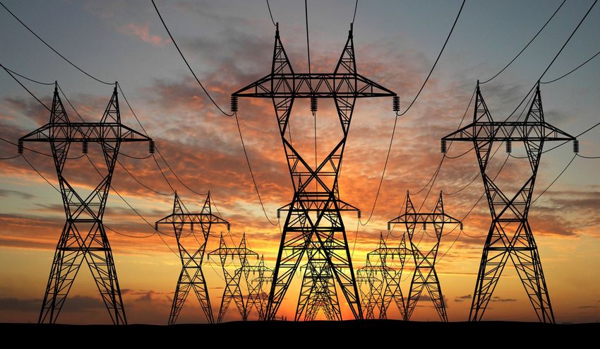
RTE is organized into seven geographical regions, as illustrated in figure 1.3. The power
system is operated by seven regional network control centers (called dispatching) located in
each of these regional areas and a centralized center called CNES (National system for System
Operation) located in Paris.
Figure 1.3: Regional dispatching centers
The CNES is the entity responsible for keeping the balance between production and con-
sumption, maintaining voltages levels and loads on the 400 kV network, and managing cross-
border electricity flows between France and its neighboring countries. In support of the CNES,
the regional centers take care of monitoring and managing voltage levels and load flows on the
EHV (225 and 400 kV) and High Voltage (63, 90 and 150 kV) network, as well as telecontrol of
high-voltage substations. The power system units enable an access to the network for customers
and development of the regional network. In case of disturbances, the control centers have to
provide back up for the CNES in order to implement countermeasures to maintain the network
integrity.
1.2.2 Expertise and system department
I did my master’s thesis in the Expertise & System Department (called DES) in Versailles which
belongs to the R&D unit of RTE. The different divisions of this department, held by around
80 people, are working on different issues related for example to the integration of renewable
energies or new technologies, the development of the network infrastructure in the upcoming
years as well as the development of software and tools. The competences of the department
Master’s Thesis report page 13CHAPTER 1. COMPANY cover both the technical field as well as the regulatory and economic aspects. For my part, I was a member of the group GPM (Provisional Handling and Maintenance - Gestion Prévisionnelle et Maintenance) which is mainly focused on voltage stability studies. Master’s Thesis report page 14
Chapter 2

Mission

2.1     Current and upcoming challenges
2.1.1    Supply-demand balance
Transmission System Operators face different challenges. The first one is the continuous in-
creasing of the consumption and more particularly the consumption peak (which was hitting
record on February 2012 [6]). The consequences of this trend are for example to make lines
and power plants reach their physical limits. An explanation of the phenomenon could be
the constant increase of households, the development of new products such as computers or
telecommunications and finally the growing of electrical heaters. Another factor is the increase
of the European countries temperature-sensitivity, which represents the impact of the climate
temperature on the electricity demand.

    This phenomenon is really disturbing, especially since the investments made on the network,
with the building of new overhead lines or the constructions of new plants, is lagging behind the
consumption speed. Then it is more difficult to predict the future consumption as the economic
growth is slowing down. Therefore the domestic demand forecasts can be only based on the
prediction of the GDP (Growth Domestic Product) growth estimates which gives a large panel
of scenarios more or less accurate.

   Finally, the fact that more than half of the fossil-fired units will be shut down in 2016 [7] as
well as the willing of some countries to end the nuclear generation will be a challenge for the
TSOs in the upcoming years to keep the balance between generation and consumption. Many
advances were made as the development of load-shedding or energy efficiency measures which
tend to reduce the consumption on a wide range. Nonetheless, the concern of the supply-demand
balance remains one of the big challenges for the future.

2.1.2    Integration of Renewable Energy
Another phenomenon, which appeared at the end of the 19th century, is imposing some changes
in the energy production. With the arrival of some issues such as the global warming, it is essen-
tial to find a new way to produce energy. The energy regulation which has known an important
evolution started in 1997 with the Kyoto Protocol [8] followed by the Copenhagen Accord [9]
in 2002. This momentum is now reaching the European Union members which have planned
CHAPTER 2. MISSION
in 2007 to reduce their gas emissions by 20% compared to 1990, improve by 20% the energy
efficiency measures, and finally integrate more than 20% of renewable energy in the mix [10].
However, TSOs have to deal with the challenging issues that come with the integration of
renewable energy units. They are usually located away from the main network and the lines
strengthening is often necessary. Then, the production intermittency and climate hazard ap-
pears as an hurdle to the development of such technologies and highlights the accute challenges
to maintain both a reliable and cost effective supply. Despite various progress in meteorological
forecasts and the fact that it is now possible to evaluate the next day production, it is very dif-
ficult to predict the three days prior production. A consequence of the randomness of wind and
solar energy is that it is unclear how to use these units to control the network’s voltages as well
as it remains complicated to adjust active or reactive power production. The non-correlation
between renewable production and the consumption is also a major. This is particularly the
case for solar units, which produce the most energy in summer whereas the consumption is
usually low [11].
2.1.3 Electricity market’s development
At the beginning of the century, we were witnessing a new phenomenon known as "the un-
bundling of electricity grids and electricity production" which allowed an effective competition
on supply and generation. This trend, which came with the liberalization of electricity indus-
try, has led to new challenges. In fact, power companies are no longer vertically integrated
(generation, distribution and retail services no longer under one business) and TSOs have to
facilitate the development of this electricity market [12].
Furthermore to ensure a smooth running of the european market, new constraints appeared
such as [12]:
• independant transmission system operators
• account unbundling for generation, transmission and distribution activities
• independant national regulators
In this new context, which enables an easy access to many players such as traders, compet-
ing suppliers or consumers, the TSOs have to manage the complexity of this new system. As
RTE is responsible for electricity imports and exports, it has the duty to manage the conges-
tion on the cross-border connections. In that way, the European TSOs have seen their network
stretched through the different interconnections. However, even if the mesh increasing provides
a mutual assitance between countries in case of shortage, this can also induce large-scale voltage
collapses in Europe, caused for example by a single disturbance in only one country. This new
particularity shows that high transparency and cooperation are now required between TSOs
and all the players.
Master’s Thesis report page 16CHAPTER 2. MISSION
2.2 Master’s thesis objectives
2.2.1 Aim of the project
The first study of this master’s thesis focuses on a new device (called SMACC) that has recently
been developed by RTE to control compensations means, due to the installation of various bat-
teries of capacitors in the South-West of France. The SMACC has already be designed by an
internal departement at RTE but a deep study regarding the presence of potential interactions
has never been done yet.
Then it has been demonstrated that the South-West is still sensitive to voltage collapse after
very severe disturbance. A second study is consequently carried out to evaluate whether an
automatic load shedding is necessary to mitigate large-scale voltage collapses. The installation
of the HVDC (High-voltage direct current) line between France and Spain has also a crucial
importance for these studies.
2.2.2 Thesis work outline
Before starting test, the SMACC is introduced in order to have a good understanding of the
context. Then the SMACC is modelised in the softwares (both Convergence and Eurostag).
The support for our simulations is the situation of the 9th of February 2012. It is necessary to
have accurate data, especially on the South-West region of France and on the spannish network,
and to calibrate both situations in Convergence and Eurostag. Then the SMACC is tested and
finally some improvements are suggested.
Regarding the load shedding device (LSD), the context of the study is given in a first part.
Then a situation at horion 2020 is studied and calibrated. The LSD is modelized and then inte-
grated into the forecasting situation. Finally different studies are conducted regarding voltage
stability by simulating different constraining defaults in the South-West region and different
setups of LSD are tested in order to avoid a general voltage collapse as efficiently as possible.
2.2.3 Outline
• The first chapter focuses on RTE where the Master’s Thesis has been done. The company
mission is presented and key figures are provided. The context of the Thesis is introduced
in the second chapter.
• Chapter 3 provides a theoretical background about voltage stability. Some notions are
given regarding the network model and the phenomenon of drop of voltage. The concept
of voltage collapse is also introduced.
• Chapter 4 descibes the software used during the Master’s Thesis.
• The SMACC and the LSD studies have been made respectively in chapter 5 and 6. In
each chapter, a presentation of the context is provided and then a part is devoted for
simulations and results.
Master’s Thesis report page 17Chapter 3
Theoretical study
3.1 Introduction of power system stability
According to CIGRE-IEEE [13]: "Power system stability is the ability of an electric power
system, for a given initial operating condition, to regain a state of operating equilibrium after
being subjected to a physical disturbance, with most system variables bounded so that practi-
cally the entire system remains intact."
The power system is continuously subjected to various disturbances and it is necessary that
TSOs maintain a high reliability of operation and a satisfactory security level, regardless the
network conditions. The latest incidents in the world, such as the one in the United States
in 1965 [14], shows the difficulty to operate the Power System. Depending on the network
topology, the system operating conditions and the form of the disturbance, the Power System
can undergo different types of instabilities. This master’s thesis focuses essentially on voltage
stability, and more precisely long-term voltage stability.
Voltage stability refers to the ability for a power system to maintain at all buses acceptable
equilibrium voltage values after a disturbance. The driving force for voltage instability is usually
the loads. In response to a disturbance, power consumed by the loads tends to be restored by
the action of motor slip adjustment, distribution voltage regulators, tap-changing transformers,
and thermostats. Restored loads increase the stress on the high voltage network by increasing
the reactive power consumption and causing further voltage reduction [13]. It can be useful to
classify voltage stability into two categories:
• Small disturbance voltage stability which defines the ability for a power system to keep
steady voltage after a small perturbation like a load gradual change. Usually, this form
of stability can be studied by linearizing the system dynamic equation.
• Large disturbance voltage stability which is concerned with a system’s ability to con-
trol voltage after large disturbances such as system faults, loss of generation, or circuit
contingencies.
The time frame of interest for voltage stability can vary from a few seconds to tens of
minutes. As a result, voltage stability can be a short-term or a long-term phenomenon.CHAPTER 3. THEORETICAL STUDY
• Short-term voltage stability, mainly involves dynamics of fast acting load components
such as induction motors or HVDC converters, particularly to their inverter terminals.
The driving force of instability is the tendency of dynamic load to restore consumed power
in the time frame of a second after a voltage drop caused by a contingency.
• Long term voltage stability involves slower acting equipment such as tap-changing trans-
formers, thermostatically controlled loads, and generator current limiters. It can be as-
sumed that the system has survived the short-term period following the initial disturbance
and the dynamic time scale can reach several minutes.
This master’s thesis focuses on long-term voltage instability. In the next sections is de-
scribed how a disturbance may lead to a voltage collapse and the different parameters that can
contribute to this type of incident are also emphasized.
3.2 Network model and performance
3.2.1 Line model
Regarding different parameters such as the length as well as the transmitted power, the line
may be represented by different models. The transmission lines are mainly classified as short,
medium or long lines. Short transmission lines (250 km) the parameters are distributed along the line which makes the analysis more
complicated. Thus, it is necessary to take into account propagation phenomena which makes
the system more complex to solve.
In order to illustrate the problematic of long-term voltage stability, a simple example is
considered and represented by a medium line with length between 80 and 250 km (most of
the lines). As a three-phase system is considered, it is possible to study only the per-phase
equivalent circuit. Its representation is described in figure 3.1.
Rl Xl
C G C G
Figure 3.1: Per-phase equivalent circuit
The different parameters of the line are:
The series resistance R : which reflects the joule losses.
The series inductance Xl : due to the magnetic field inside and outside the conductor
Master’s Thesis report page 19CHAPTER 3. THEORETICAL STUDY
The shunt capacitance C : due to the difference of potential between conductors
The shunt conductance G : which modelizes the corona effect.
Below are given some magnitude examples:
R : 3Ω/100km
Xl : 30Ω/100km
C : 1.2µF/100km
G : 1.2nS/100km
In our case, the shunt conductance is neglected given the medium line model, as shown in
figure 3.2. Then, for high transmitted power, the current may reach high values and it is then
possible to neglect also the shunt capacitance in favour of the series inductance.
Rl Xl
I
V1 V2 Zch
Figure 3.2: Symplified model
For the study, the generator will be considered as a slack bus (with a constant output volt-
age and without any power limitations). The load is both resistive and inductive. Furthermore,
the line is not lossless (the line resistance is taken into account).
V1
∆V
θ
φ V2
I
Figure 3.3: Vector diagram
First of all, we can start by defining the line impedance Z as well as the voltage difference
between the sending and receiving end ∆V :
Master’s Thesis report page 20CHAPTER 3. THEORETICAL STUDY
Z = Rl + jXl (3.1)
∆V = ZI = V1 − V2 (3.2)
Now, let P2 and Q2 be the active and reactive power loads, respectively. We can introduce
in the same way φ, the phase shift between V2 and I.
P2 = V2 Icosφ (3.3)
Q2 = V2 Isinφ (3.4)
P2 − jQ2
I= (3.5)
V2
We can now develop the equation (3.2) :
V1 = V2 + Rl I + jXl I (3.6)
∆V = ZI = (Rl + jXl )(P2 − jQ2 )/V2 (3.7)
Rl P2 + Xl Q2 Xl P2 − Rl Q2
= +j (3.8)
V2 V2
= ∆Vr + j∆Vx (3.9)
V1
∆V ∆Vx
θ
V2 ∆Vr
Figure 3.4: Vector diagram
From this, it can be noticed that the voltage drop is composed of two components :
• ∆Vr : the radial part
• ∆Vx : the quadratic part
|V1 |2 = (V2 + ∆Vr )2 + ∆Vx2 (3.10)
∆Vx
sinΘ = pCHAPTER 3. THEORETICAL STUDY
Then, it is possible to neglect the quadratic part of the equation 3.9, and the voltage drop
induced by the line is:
Rl P2 + Xl Q2
∆V = (3.12)
V2
Now, if we still consider a high transmitted power value, the series resistance can be ne-
glected:
Rl P2 + Xl Q2 Xl Q2
∆V = ≈ (3.13)
V2 V2
This results shows us that the drop of voltage is mainly caused by the reactive power
consumed by the load. Therefore, in order to keep V2 constant, it is necessary to apply a
variable reactive power production at the receiving point.
3.2.2 Maximal transmissible active power
In order to symplify the problem, only the line inductance is considered and the load will be
considered as purely resistive.
Xl
I
V1 V2 R
Figure 3.5: Simple line model
∆V = ZI = Xl I (3.14)
Then, we can symplify the expression of the power consumed by the load and find out the
expression of I, since φ equals 0 now.
P2 = V2 Icosφ = V2 I (3.15)
V1 = V2 + Rl I + jXl I (3.16)
|V1 |2 = |V2 |2 + |Xl I|2 (3.17)
q
V12 − V22
I= (3.18)
Xl
Master’s Thesis report page 22CHAPTER 3. THEORETICAL STUDY
V1
∆V
θ
I
V2
Figure 3.6: Vector diagram
From (3.15) and (3.18):
V2 q 2
P2 = V1 − V22 (3.19)
Xl
Now we can plot the curve of V2 as a function of P2 :
V2
b
Va
b
V2c
b
Vb
P0 Pmax P2
Figure 3.7: Nose curve
From this diagram, we can highlight three remarkable points. The first two points Va and
Vb corresponds to the two operating points of the line for a given power. It means that for the
same transmitted power it is mathematically possible to operate the system at two different
voltages. However, the system never operates at the lowest voltage Vb since the line current is
three times higher and so the reactive losses are much higher.
Master’s Thesis report page 23CHAPTER 3. THEORETICAL STUDY
V2c is another operating point and corresponds to the voltage of maximal power, also known
as the critical point. In order to find the value of V2c and Pmax , it can be useful to express the
transmitted power as a function of the power angle θ:
V1 ∗ V2
P2 = sinθ (3.20)
Xl
Since,
V2 = V1 cosθ (3.21)
We can express the receiving power as below:
V1 ∗ V1 V2
P2 = sinθcosθ = 1 sin2θ (3.22)
Xl 2Xl
From (3.22), it can be concluded that P2 is maximal when θ = π4 :
V12
Pmax = (3.23)
2Xl
Where,
V1
V2 = √ (3.24)
2
This diagram also shows us that when the load exceeds a specific limit, the receiving voltage
drops considerably and the receiving power decreases. This confirms the fact that the lower
part of the diagram is an instable operating part of the system. Now if we consider a pure re-
sistive load, we can derive another expression of the receiving voltage as a function of the power:
V22
P2 = (3.25)
R
The intersection of both curves in figure 3.8 gives a unique operating point. The operating
power is lower than the maximal transmittable power and the operating voltage is also lower
than the critical point which means that the system is operating in good conditions.
3.2.3 Reactive loss
As mentionned previously, the reactive variation can be divided by two terms:
• The reactive consumption, linked to the line inductance
Master’s Thesis report page 24CHAPTER 3. THEORETICAL STUDY
V2
Vop
b
b
V2c
Pmax P2
Figure 3.8: Nose curve : operating point
Rl Xl
C C
Figure 3.9: Π Model
• The reactive supply, due to the shunt capacitance
It then possible to express the total reactive losses as:
Qlosses = 3Xl I 2 − 3CωV22 (3.26)
By supposing that the line voltage remains almost constant, the reactive losse is an increas-
ing function of the line current, as represented in figure 3.10.
When the current on the line is very low, the line reactive supply due to the shunt capaci-
tance is higher than the reactive consumption caused by the line inductance. As a consequence,
the line is supplying reactive power. When the current increases and so the complexe power,
the line inductance tends to increase the reactive consumption, therefore the reactive losses
Master’s Thesis report page 25CHAPTER 3. THEORETICAL STUDY
Qloss
1000
800
Qloss = 3Xl I 2 − 3CV22
600
400
200
0
500 1000 1500 2000 2500 S
−200
Figure 3.10: Reactive loss
increase. In case the complexe power equals around 500 MVar, the reactive supply and the
reactive consumption of the line are almost the same. The highest the current is (and so the
active power) and the highest are the reactive losses. Since the evolution of the losses is pro-
portionnal to the square of the current, it is then really necessary to distribute the active power
flows on a maximum of lines.
3.2.4 Influence of some parameters
Voltage Source V1
The sending voltage has a large influence on both the receiving voltage and on the maximal
transmissible power. The expression of the receiving active power is (3.19) as demonstrated
in 3.2.2. On the figure 3.11, differents curves have been ploted with different sending voltage
value. (For each curve the line inductance has the same value).
It worth noticed that the value of V2 increases with the voltage source V1 . Then, we can
also notice that a higher sending voltage leads to a higher maximal transmissible power and
therefore the power margins are increased for a given load power.
Line reactance Xl
We have seen that the drop of voltage and the transmissible power can be respectively expressed
by 3.13 and 3.19. Both equations show us that the series inductance value has a huge influence
on system reliability. Firstly, the value of the drop of voltage is high if the inductance line is
high in the same way. Secondly, the maximal power is lower if the inductance line is higher.
The diagram 3.12 represents 3 power curves each with a different value of Xl (V1 is fixed now).
Master’s Thesis report page 26CHAPTER 3. THEORETICAL STUDY
V2
V1 = 1.1pu
V1 = 1pu
V1 = 0.9pu
P2
Figure 3.11: Impedance influence
We can notice that the inductance has an opposite effect to V1 . For a given load power,
the receiving voltage is lower if the inductance is higher. Then, a high value of the inductance
induces a low maximal power. We conclude that it is preferable to operate the system with a
low value of Xl in order to avoid an important voltage drop.
Load impedance Z
In order to evaluate the load impedance impact on the system, we cannot consider a purely
resistive load anymore. We still consider a perfect generator and a purely inductive line (see
figure 3.5). We have already expressed the transmitted power as a function of the power angle
in equation (3.20). It then possible to express the transmitted reactive power Q2 as a function
of the power angle.
V1 V2 V2
Q2 = cosθ − 2 (3.27)
Xl Xl
By combining equations (3.20) and (3.27), we can derive the expression of the receiving
power as a function of the tangente φ and the receiving voltage [15]:
s
V22 [1 + (tanφ)2 ]V12
P2 = [−tanφ + −1 + ] (3.28)
Xl (1 + (tanφ)2 ) V22
From (3.28), we can derive the maximal loadability as follows:
V12
Pmax = (1 − sinφ) (3.29)
2.Xl .cosφ
s
V1 (1 − sinφ)
Pmax = (3.30)
cosφ 2
Master’s Thesis report page 27CHAPTER 3. THEORETICAL STUDY
V2
Xl′
Xl
V1
√
2
Xl′′
Xl′ < Xl < Xl′′
P2
Figure 3.12: Reactance influence
On the figure 3.13, some nose curves are ploted with different values of tanφ.
First, we can notice that the decrease in the algebric value of tanφ tends to increase the
system operating voltage point. The line has more capacity and for a given power flow, the
voltage is higher. When the voltages are quite low, especially in winter, it is possible to use
shunt capacitors on the supply substations to increase the receiving voltage [16]. However an
important decrease in the tanφ, by means of compensation, may lead to some instability since
the operating voltage value is getting closer to the critical voltage value.
Generator limitations
For the previous studies we have considered a generetor with no limitations. However, it is
not the case in reality since the generators do not have unlimited power reserves. It is possible
to represent a synchronous generator by the following equivalent circuit (here the transmission
line is not represented) as shown in figure 3.14.
Where:
• E is the generated voltage
• Xs is the synchronous reactance
• I is the current
The operating domain of the generator faces different limits such as current or turbine power
limitations induced by rotor or stator heating limits. We usually study a generator on a [P,Q]
diagram for a given stator voltage, as shown in figure 3.15.
Master’s Thesis report page 28CHAPTER 3. THEORETICAL STUDY
V2
−0.5
−0.3
0
0.3
P2
Figure 3.13: Impedance influence
Xs
I
E
E∠δ jXs I
δ
V
θ
V
I
Figure 3.14: Generator equivalent circuit and phasor diagram
Generators connected to the grid are equiped with different protections and regulation de-
vices that prevent the different values of exceeding the limitations. As we are studying the
potential risk of voltage collapse, the only limitation that we will take into account is the rotor
current limitation since it is directly related to the generator capacity of reactive supply. When
this limitation is reached, a protection loop ensures that the generator to decrease the voltage
while maintaining a constance reactive supply.
In order to evaluate the impact of this limitation, we still use the simple line model as the
one in section 3.2.2, but we take now into account the maximal reactive power production.
We can express the formula linking the generator reactive power production Q1 , the receiving
voltage V2 and power P2 .
The expression of the transmitted power P2 has already been given in equation (3.20). We
can also express the reactive power production from diagram 3.6:
Q1 = V1 Isinθ (3.31)
Master’s Thesis report page 29CHAPTER 3. THEORETICAL STUDY
Figure 3.15: Generator operating limitations on a P-Q diagram [17]
Where V1 sinθ = ∆V
∆V 2
Q1 = I.∆V = (3.32)
Xl
From (3.20) and (3.32), we can derive the formula linking V2 , P2 and Q1 :
s
Xl
V2 = P2 (3.33)
Q1
The impact of the generator limitation has been represented on the diagram 3.16.
They are two possible scenarios:
• Irotor < Ilimitation : The generator didn’t reach its reactive supply limitation yet and the
curve follows the nose curve described by the equation (3.19).
• Irotor = Ilimitation : The generator cannot produce more reactive power and the system
follows the equation (3.33). V2 starts to decrease in inverse proportion to the increase
of the demand. The maximal transmitted power decreases and the system is much less
stable.
Master’s Thesis report page 30CHAPTER 3. THEORETICAL STUDY
V2
P2
Figure 3.16: Rotor current limitation
3.2.5 Load modeling
There are various types of loads in power systems as shown in figure 3.17. The load character-
istics at each substation should represent properly the aggragete effect of all loads connected,
especially since these models are directly taken into account for power flows or stability studies.
Figure 3.17: Loads classification [18]
The first designed load models failed to bring a good understanding of some phenomena
Master’s Thesis report page 31CHAPTER 3. THEORETICAL STUDY
such as voltage collapses since they were not accurate enough [18]. Furthermore, different load
models could give very large results differentials which emphasize the need for a more accurate
model.
In addition, it is important to differ static load modeling and dynamic load modeling. For
example a high proportion of the load is represented by induction motors and the behavior of
such loads can only be explained through dynamical models. Static models are mostly used
for steady state conditions calculations, and dynamic models for studying dynamic phenomena
[19]. A brief introduction of dynamic load modeling is made in this chapter.
Static load models
Static load models are generally defined as a function of the active and reactive power, which
depend on the voltage and the frequency.
U α ω δ
P = P0 ( ) ( ) (3.34)
U0 ω0
U β ω γ
Q = Q0 ( ) ( ) (3.35)
U0 ω0
P0 and Q0 are respectively the active and reactive loads computed through the load flow
computations. U0 is the busbar voltage at initial state and ω0 the frequency.
Since the characteristics of the loads are not the same and so don’t have the same voltage
sensitivity, the coefficients may differ between different loads, as shown in figure 3.18.
Models α β
constant power 0 0
constant current 1 1
constant impedance 2 2
Figure 3.18: Static load models
A combination of these models is generally used to represent the loads, known as the poly-
nomial representation [20]:
U 1 U
P = P0 [a1 + a2 ( ) + a3 ( )2 ] (3.36)
U0 U0
U 1 U
Q = Q0 [a4 + a5 ( ) + a6 ( )2 ] (3.37)
U0 U0
Where V0 , P0 and Q0 are the values at the initial conditions and the coefficients a1 to a6
are the parameters of the system.
We can notice that the results of a stability study are different regarding the coefficients
taken in the equations 3.36 and 3.37, so it is important to have an accurate model which reflects
Master’s Thesis report page 32CHAPTER 3. THEORETICAL STUDY
reality as well as possible.
Figure 3.19: Influence of the static load characteristics [20]
Figure 3.19 shows us the influence of static load models on the nose curve after a disturbance
(line tripping for instance). We can notice that when α is decreasing, the new operating point
is closer to the critical point and so voltage stability is more affected. This is particularly the
case when α equals −0.5.
Dynamic load models
We have studied in the first section the static load models which gives a good overview of the
loads behavior. However, some loads such as electric heating would tend to recover the initial
power (at the pre-disturbance state) after the drop of voltage induced by the line tripping. An
approach of this dynamic response can be represented by the equations 3.38 and 3.39, [19].
dPr U U
Tp + Pr = P0 ( )αs − P0 ( )αt (3.38)
dt U0 U0
U αt
Pl = Pr + P0 ( ) (3.39)
U0
Where U0 and P0 are the voltage and the consumption at the initial conditions, Pr is the
active power recovery, Pl is the total active power, Tp is the active load recovery time constant,
αt is the transient active load-voltage dependence and αs is the steady state active load-voltage
dependence. An approach of the load evolution after disturbance is represented in figure 3.20.
The power increasing can be seen by a decreasing of the coefficient α. However, it α decreases
too much, there is a risk that the requesting power becomes higher than the critical point of
the figure 3.19.
Master’s Thesis report page 33CHAPTER 3. THEORETICAL STUDY
Figure 3.20: Load response under voltage drop[19]
3.3 Voltage control mechanisms
3.3.1 Introduction
We have seen in the section 3.2 that it is important to control voltage, in order to maintain sup-
ply voltage within contractual agreement or to respect the various equipment constraints, and
also to minimize losses and use the capacity of power facilities as well as possible. The voltage
drop is really dependent on reactive power flows, therefore to control the voltage it is necessary
to compensate in the same way the reactive power. This is the role of load compensation to
improve the quality of supply in ac power systems [21], whose 3 main objectives are:
• Power-factor correction
• Improvement of voltage regulation
• Load balancing
In that way we could define the ideal compensator as the device capable of performing those
three functions, with an ability to respond instantaneously to variations. It means that this
capacitor would have the property to provide a controllable and variable amount of reactive
power, would present a constant voltage at its terminal and would be able to operate indepen-
dently in the three phases.
It exists today different types of compensating equipments each with specific properties. For
instance, the compensation on the distribution network (on the supply substations) is mainly
made from shunt capacitors. Regarding the transmission network, the reactive power compen-
sation is mainly ensured by the connected generators. However, since production is usually
far from the load, it is also necessary to use passive control equipments such as capacitors on
Master’s Thesis report page 34CHAPTER 3. THEORETICAL STUDY
the transmission grid in order to relieve the groups action and to offer more power capability
through the lines. When the transmission network tends to be rather reactive power producer,
the use of reactors can be needed. Finally, synchronous condensers are effective control devices
which have the possibility to both supply or absorb variable reactive power.
The generators reponse time is very short and therefore they can adapt instantly their
reactive power supply in a very precisely. On the contrary, capacitors which have a much
longer response time, are mainly used to follow periodical fluctuations. Then it is important
to precise that the reactive power production from a capacitor decreases proportionnaly to the
square of the voltage. The generators regulation is supervised by three levels of voltage control
that are spatially and temporally independent in order to avoid contradictions between the
different actions conducted:
• Primary Voltage Control: All generators are equipped with a primary voltage controller
which gives them the ability to control their stator voltage at set points, by varying their
excitation current. Obviously this control is operational within the constructive limit of
the generators. This automatic device has a very fast response time and is therefore the
most efficient mean of voltage control, particularly to deal with random load fluctuations.
• Secondary Voltage Control: The Primary Voltage Control is a purely local mechanism and
a centralized control is consequently necessary to coordinate the actions of the network’s
generators. In fact, after a disturbance, the local regulation enables the generators to
adjust their stator voltage but it is usually a non optimum solution for the overall network,
where a generator may for example produce reactive power partially absorbed by another
one. Contrary to the primary voltage control, the time-scale of this mechanism is around
few minutes.
• Tertiary Voltage Control: The last voltage control aims to rehabilitate secondary voltage
set point levels following the continuous changes of operating conditions. Thus it enables
the system to be operated at an economic optimum and avoid also degraded network
operation. It is usually a manual process but it can be automatized with a time-scale of
at least 15 minutes.
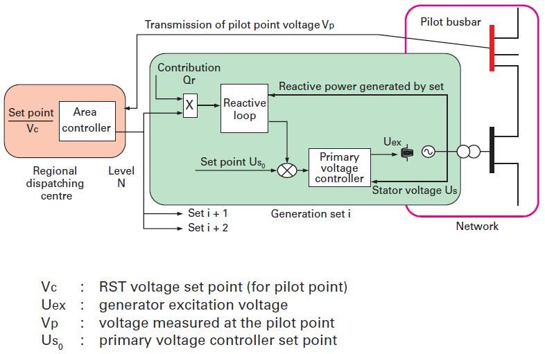
3.3.2 Secondary Voltage Control
As shown in figure 3.21, the main interest of the Secondary Voltage Control (SVC) is to control
the voltage value inside a specific geographical area. A pilot point is defined in each area and
if the pilot point voltage differs from the set point voltage, an automatical order is sent to the
groups which belong to the area in order to adjust their reactive power production. Generally
speaking, this is a set of generators controlling by a pilot point that defines a SVC area.
In France, there are 35 pilot points and the voltage control in a specific area is totally
independent from the others. Then a pilot point should be sufficiently representative of the
overall area and shouldn’t be too close of the units. For each zone a signal N, which represents
the required reactive power level for the zone, is computed in the regional control centers by
applying a proportionnal integral law to the difference between the pilot point set-point voltage
and the pilot point voltage measurement. Then this level N is sent to all the units every 10
Master’s Thesis report page 35CHAPTER 3. THEORETICAL STUDY
Figure 3.21: Secondary Voltage Control [22]
seconds and is used to determine a set-point for the reactive power loop of each unit, as shown
in figure 3.21. The reactive power loop increases or decreases the terminal voltage set-point
of the primary voltage controller, regarding the input parameters such as the level N or the
current reactive power production of the generator.
Thus the SVC enables to increase the efficiency of the Primary Voltage Controller and also
to coordinate the groups actions in a same area, particularly after a disturbance. It is then
possible to get the steady-state reactive power generation aligned, as long as a generator limit
is not reached. However, the Secondary Voltage Control has also some drawbacks:
• The level N sent to the generator is exactly the same (for a given area) which is usually not
the best optimum regarding the economic or the safety aspects. This is especially the case
when a generator reaches its physical limitations (such as the rotor current limitation)
and doesn’t participate anymore to the secondary control.
• The parameters of the reactive loop are fixed and should be adapted regarding the oper-
ating conditions.
• The SVC presents also an adverse effect on the reactive loop which is slower than the pri-
mary control and which sometimes delays the reactive power production of the generator
after a disturbance.
A new Secondary Voltage Control has been developed in order to eliminate these different
drawbacks. This new mechanism is the Coordinated Secondary Voltage Control (CSVC). At
this moment, the CSVC was implemented only in the Western are of the frend grid, in the
regional control center, since this is the part of the network where the voltage constraints
are the most important. The new control, contrary to SVC, has the possibility to adjust the
voltage map of a given region by regulating the voltage values at a set of pilots points. The
CSVC computes directly, for each group, the terminal voltage variations to apply at its Primary
Voltage Regulator. The CSVC used an algorithm whose main variables are :
Master’s Thesis report page 36CHAPTER 3. THEORETICAL STUDY
• the difference between pilot points voltage and their set-point value
• the difference between each group’s reactive power production/stator voltage and their
set-point values
While taking into account:
• the network constraints
• the groups operating diagram
• the possible set-point variations of the primary regulator
As a result, the major interactions between areas are taken into account, and the adverse
effect of the reactive loop doesn’t intervene anymore since the set-point voltage is directly
computed at the control center and then sent to the groups. The voltage map is also more
stable and more accurate following disturbances. The dynamic of the mechanism is also much
faster than the former one.
3.3.3 On-load tap changers
Another system widely used to control the voltage is the On-Load Tap Changer (OLTC). In
order to fullfill the requirement in terms of electricity quality, and since these requirements are
not the same in the transmission and the distribution grid, it is necessary to decouple as well as
possible those two networks. The OLTC enables to keep the distribution voltages in a suitable
range independently of the voltage variations in the transmission grid.
Practically all power transformers and many distribution transformers are equipped with
On-Load Tap Changer which enables them, while being on duty, to change their turns ratio
tr between windings and therefore to control the transformer output voltage, as shown in fig-
ure 3.22. In that way, the transformers have taps, in one or several winding, bounded by an
upper limit and a lower limit, and connected to the OLTC. By varying the tap position, the
turns ratio tr of the transformer can be changed and therefore the secondary voltage is contin-
uously adjusted.
At every moment, the secondary voltage is compared to the set-point value. If the voltage
measurement is lower (respectively higher) than the requirements, the OLTC is engaged. After
a certain time, which varies regarding the voltage levels where the transformers are connected
to, the tap number increases (decreases) one by one, and this operation is repeated until the
voltage measurement matches the half-deadband or until the OLTC reaches one of the limits.
At any moment we have:
• V3 = V2 /tr = VLoad if the OLTC is operating between its limits
• V3 = V2 /trmax if the OLTC reaches the lower limit
Master’s Thesis report page 37You can also read