Development and performance evaluation of undertray diffusers during racing manuevers
←
→
Page content transcription
If your browser does not render page correctly, please read the page content below
Development and performance
evaluation of undertray diffusers
during racing manuevers
Bachelor’s thesis in Mechanics and Maritime Sciences

WILLEM DE WILDE
JACOB GUNNARSSON
LENA IVARSSON
LINNÉUS KARLSSON
OSKAR KOLTE
DANIEL OLANDER

DEPARTMENT OF MECHANICS AND MARITIME SCIENCES
C HALMERS U NIVERSITY     OF   T ECHNOLOGY
Gothenburg, Sweden 2021
www.chalmers.se
Bachelor’s thesis 2021:12

Development and performance evaluation of
undertray diffusers during racing manuevers

                  WILLEM DE WILDE
                 JACOB GUNNARSSON
                    LENA IVARSSON
                  LINNÉUS KARLSSON
                     OSKAR KOLTE
                   DANIEL OLANDER

        Department of Mechanics and Maritime Sciences
    Division of Vehicle Engineering and Autonomous Systems
           Chalmers University of Technology
                    Gothenburg, Sweden 2021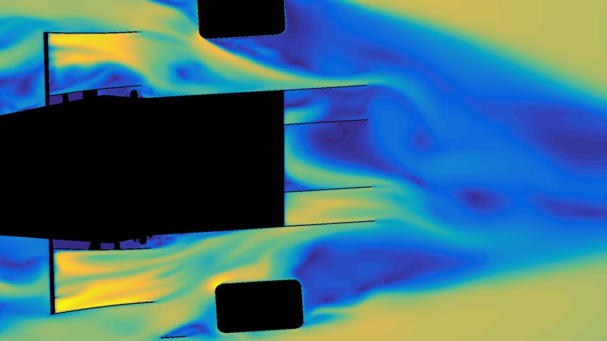
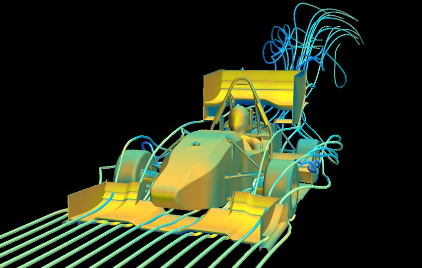
Development and performance evaluation of undertray diffusers during racing manuev-
ers

WILLEM DE WILDE
JACOB GUNNARSSON
LENA IVARSSON
LINNÉUS KARLSSON
OSKAR KOLTE
DANIEL OLANDER

© WILLEM DE WILDE, JACOB GUNNARSSON, LENA IVARSSON, LINNÉUS
KARLSSON, OSKAR KOLTE, DANIEL OLANDER, 2021.

Supervisor: Erik Josefsson, Division of Vehicle Engineering and Autonomous Sys-
tems
Examiner: Simone Sebben, Division of Vehicle Engineering and Autonomous Sys-
tems

Bachelor’s Thesis 2021
Department of Mechanics and Maritime Sciences
Chalmers University of Technology
SE-412 96 Gothenburg
Telephone +46 31 772 1000

Cover: Velocity streamlines around the Chalmers Formula Student car and Cp
visualized on the surface while driving straight.

Typeset in LATEX, template by Magnus Gustaver
Printing /Department of Mechanics and Maritime Sciences
Gothenburg, Sweden 2021

iv
Abstract
A potential to develop the monocoque and diffuser on the Chalmers Formula Stu-
dent (CFS) car, as to increase its downforce, was identified by CFS. Downforce is
the downward aerodynamic lifting force that is obtained when a pressure difference
is created between the top and bottom of the car. This effect is crucial for the grip
of the car in driving scenarios like cornering, accelerating and braking. With more
downforce, accelerating and braking can be done faster, and higher speeds can be
maintained in cornering.

The objective of this project is to develop a methodology for modeling of aerody-
namic forces during different racing maneuvers of a CFS car. These new methods
are purely computational. Further, the methods are used in the development of a
new diffuser concept. This is done with the aim of providing CFS with knowledge
and proof-of-concept of the implementation of a new diffuser, which could increase
aerodynamic performance of the car.

It was shown that straight ahead driving, braking, and cornering were the most
critical driving scenarios. These were used to perform three types of simulations.
Different diffuser designs were simulated based on these scenarios. It was further
shown that the following parameters had an effect on aerodynamic performance: the
expansion angle of the diffuser, the starting point of the diffuser, the radius of the
diffuser throat, and the implementation of strakes and side floors. Differences in the
performance robustness of the different designs were observed.

Two diffusers provided the greatest downforce: one with a 13° expansion angle
and the other with a 19° expansion angle. The diffusers were in other regards iden-
tical. Lastly, the 13° diffuser was chosen as the best contending design, due to its
robust performance in each of the simulated driving scenarios.

Keywords: CFD, aerodynamics, Formula Student, downforce, lift coefficient, drag
coefficient, diffuser, racing manuevers, cornering, braking.

                                                                                    v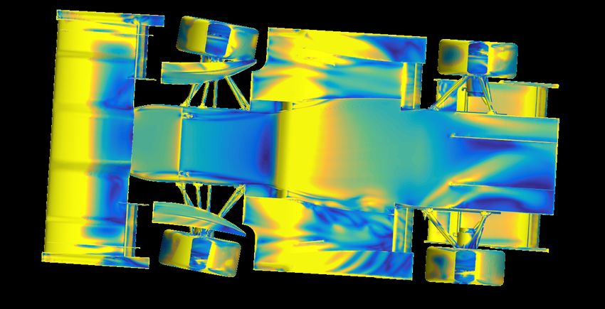
Sammandrag
En potential att vidareutveckla monocoque och diffusor på Chalmers Formula Student-
bilen (CFS-bilen), med avsikt att öka bilens downforce, identifierades av CFS. Down-
force kallas den nedåtriktade aerodynamiska lyftkraft, som uppstår vid en tryckskill-
nad mellan bilens ovan- och undersida. Denna effekt är avgörande för bilens grepp
i körscenarier såsom kurvtagning, acceleration och inbromsning. Större downforce
tillåter kraftigare acceleration och inbromsning och att högre hastighet kan hållas
under kurvtagning.

Detta projekts syfte är att utveckla en metodik för att modellera aerodynamiska
krafter under de olika manövrar som en CFS-bil gör under en tävling. Dessa metoder
är baserade på simuleringar. Vidare ska metoderna användas för att assistera utveck-
lingen av ett nytt diffusor-koncept. Detta görs med målet att tillhandahålla CFS
kunskap om, och konceptvalidering för implementeringen av en ny diffusor, vilket
kan förbättra bilens aerodynamiska prestanda.

Det visades att rak körning, inbromsning och kurvtagning var de mest kritiska
körscenarierna. Tre typer av simulering baserades på dessa scenarier. Olika typer
av diffusorer undersöktes med dessa simuleringstyper. Vidare visades att följande
parametrar hade en inverkan på bilens prestanda: diffusorns expansionsvinkel, dif-
fusorns övergångsradie, samt implemetering av skiljeväggar och sidogolv. Skillnader
i de olika diffusorernas prestandas robusthet observerades.

Två diffusorer genererade störst downforce: en med expansionsvinkeln 13°, och den
andra med expansionsvinkeln 19°. I andra hänseenden var diffusorerna identiska.
Slutligen valdes diffusorn med 13° expansionsvinkel som den bäst presterande av de
undersökta. Detta baserades på dess robusta prestanda i alla undersökta körscenar-
ier.

Nyckelord: CFD, aerodynamik, Formula Student, downforce, lyftkraftskoefficient,
motståndskoefficient, diffusor, manövrar, kurvtagning, inbromsning.

vi
Acknowledgements
We would like to express our greatest gratitude to our supervisor Erik Josefsson,
Ph.D student in the Road Vehicle Aerodynamics research group, for all the help and
guidance throughout this bachelor thesis.

We would also like to thank Simone Sebben, professor in Aerodynamics and manager
of the division Vehicle Engineering and Autonomous Systems, for the opportunity
to carry out this thesis. Simone Sebben has given us lectures that have been very
useful in the project.

Finally we would like to thank the Chalmers Formula Student 2021 team for their
cooperation. We are particularly grateful for Christian Svensson’s invaluable source
of knowledge and willingness to help in this project.

                                              The authors, Gothenburg, May 2021

                                                                                 vii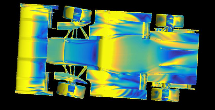
viii
Contents

Nomenclature and Abbreviations                                                                                                           xiii

List of Figures                                                                                                                          xv

List of Tables                                                                                                                           xix

1 Introduction                                                                                                                             1
  1.1 Historical Background      .   .   .   .   .   .   .   .   .   .   .   .   .   .   .   .   .   .   .   .   .   .   .   .   .   .     2
  1.2 Objective . . . . . . .    .   .   .   .   .   .   .   .   .   .   .   .   .   .   .   .   .   .   .   .   .   .   .   .   .   .     2
  1.3 Working Methods . . .      .   .   .   .   .   .   .   .   .   .   .   .   .   .   .   .   .   .   .   .   .   .   .   .   .   .     3
  1.4 Delimitations . . . . .    .   .   .   .   .   .   .   .   .   .   .   .   .   .   .   .   .   .   .   .   .   .   .   .   .   .     3

2 Theory                                                                                                                                   5
  2.1 Fundamental Fluid Dynamics Theory . . . . . . . . . . .                                                .   .   .   .   .   .   .     5
      2.1.1 Bernoulli’s Principle and the Continuity Equation                                                .   .   .   .   .   .   .     5
      2.1.2 Dimensionless parameters . . . . . . . . . . . . .                                               .   .   .   .   .   .   .     5
             2.1.2.1 Reynolds Number . . . . . . . . . . . .                                                 .   .   .   .   .   .   .     6
             2.1.2.2 Drag Coefficient, CD . . . . . . . . . . .                                              .   .   .   .   .   .   .     6
             2.1.2.3 Lift Coefficient, CL . . . . . . . . . . . .                                            .   .   .   .   .   .   .     6
             2.1.2.4 Pressure Coefficient, Cp . . . . . . . . .                                              .   .   .   .   .   .   .     6
             2.1.2.5 Skin Friction Coefficient, Cf . . . . . . .                                             .   .   .   .   .   .   .     6
      2.1.3 Vorticity . . . . . . . . . . . . . . . . . . . . . . .                                          .   .   .   .   .   .   .     7
      2.1.4 Navier-Stokes Equations . . . . . . . . . . . . . .                                              .   .   .   .   .   .   .     7
      2.1.5 RANS . . . . . . . . . . . . . . . . . . . . . . . .                                             .   .   .   .   .   .   .     7
      2.1.6 Flow Past Boundary . . . . . . . . . . . . . . . .                                               .   .   .   .   .   .   .     7
             2.1.6.1 Flow Separation . . . . . . . . . . . . .                                               .   .   .   .   .   .   .     7
             2.1.6.2 The Logarithmic Overlap Law . . . . . .                                                 .   .   .   .   .   .   .     8
  2.2 CFD Theory . . . . . . . . . . . . . . . . . . . . . . . . .                                           .   .   .   .   .   .   .     9
      2.2.1 Finite Volume Method . . . . . . . . . . . . . . .                                               .   .   .   .   .   .   .     9
      2.2.2 The k −  Turbulence Model . . . . . . . . . . . .                                               .   .   .   .   .   .   .     9
      2.2.3 The k − ω Turbulence Model . . . . . . . . . . .                                                 .   .   .   .   .   .   .     9
      2.2.4 The SST k − ω Model . . . . . . . . . . . . . . .                                                .   .   .   .   .   .   .     9
  2.3 Vehicle Dynamics Theory . . . . . . . . . . . . . . . . .                                              .   .   .   .   .   .   .     9
      2.3.1 Steering Angle . . . . . . . . . . . . . . . . . . .                                             .   .   .   .   .   .   .    10
      2.3.2 Body Slip Angle . . . . . . . . . . . . . . . . . . .                                            .   .   .   .   .   .   .    10
      2.3.3 Pitch Angle . . . . . . . . . . . . . . . . . . . . .                                            .   .   .   .   .   .   .    11
      2.3.4 Roll Angle . . . . . . . . . . . . . . . . . . . . . .                                           .   .   .   .   .   .   .    11

                                                                                                                                          ix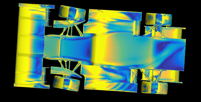
Contents

          2.3.5 Ride Height . . . . . . . . . . . . . . . . . . . . . . .                     .   .   .   .   .   12
          2.3.6 Aerodynamic Influence on Vehicle Dynamics . . . . .                           .   .   .   .   .   12
    2.4   Working Principles of a Race Car Diffuser . . . . . . . . . .                       .   .   .   .   .   13
          2.4.1 Effect of Different Design Parameters of the Diffuser                         .   .   .   .   .   14
                2.4.1.1 Differences in the Angles of the Diffuser . .                         .   .   .   .   .   14
                2.4.1.2 Differences in Area Ratio . . . . . . . . . .                         .   .   .   .   .   14
                2.4.1.3 Implementation of Strakes . . . . . . . . . .                         .   .   .   .   .   15
                2.4.1.4 Different Throats of the Diffuser . . . . . .                         .   .   .   .   .   15
          2.4.2 Venturi Vortices . . . . . . . . . . . . . . . . . . . . .                    .   .   .   .   .   15

3 Methods                                                                                                         17
  3.1 CAD       . . . . . . . . . . . . . . . . . . . . . . . . . . . . .             .   .   .   .   .   .   .   17
      3.1.1      Current diffuser . . . . . . . . . . . . . . . . . . .               .   .   .   .   .   .   .   18
      3.1.2      Design Methodology . . . . . . . . . . . . . . . .                   .   .   .   .   .   .   .   18
  3.2 CFD       . . . . . . . . . . . . . . . . . . . . . . . . . . . . .             .   .   .   .   .   .   .   20
      3.2.1      Whole-car Versus Half-car Symmetry Simulation .                      .   .   .   .   .   .   .   20
      3.2.2      Physics Model . . . . . . . . . . . . . . . . . . . .                .   .   .   .   .   .   .   20
      3.2.3      Mesh . . . . . . . . . . . . . . . . . . . . . . . . .               .   .   .   .   .   .   .   21
                 3.2.3.1 Surface Wrapper . . . . . . . . . . . . .                    .   .   .   .   .   .   .   21
                 3.2.3.2 Volume Mesh . . . . . . . . . . . . . . .                    .   .   .   .   .   .   .   21
          3.2.4 Boundaries . . . . . . . . . . . . . . . . . . . . .                  .   .   .   .   .   .   .   23
          3.2.5 Simulation . . . . . . . . . . . . . . . . . . . . . .                .   .   .   .   .   .   .   24
          3.2.6 Post Processing . . . . . . . . . . . . . . . . . . .                 .   .   .   .   .   .   .   24
    3.3   Choice of Simulated Driving Scenarios . . . . . . . . . .                   .   .   .   .   .   .   .   24
          3.3.1 Assertion of Reynolds-independence . . . . . . . .                    .   .   .   .   .   .   .   26
          3.3.2 Driving Straight Ahead . . . . . . . . . . . . . . .                  .   .   .   .   .   .   .   26
          3.3.3 Cornering Driving Scenario . . . . . . . . . . . .                    .   .   .   .   .   .   .   27
          3.3.4 Braking Driving Scenario . . . . . . . . . . . . . .                  .   .   .   .   .   .   .   28

4 Results and Analysis                                                                                            29
  4.1 General Differences for Driving Scenarios . . .         .   .   .   .   .   .   .   .   .   .   .   .   .   29
      4.1.1 Differences in Velocity Magnitude . . .           .   .   .   .   .   .   .   .   .   .   .   .   .   32
      4.1.2 Differences in Pressure Coefficient . . .         .   .   .   .   .   .   .   .   .   .   .   .   .   35
      4.1.3 Differences in Skin Friction Coefficient          .   .   .   .   .   .   .   .   .   .   .   .   .   38
      4.1.4 Differences in Vorticity Magnitude . .            .   .   .   .   .   .   .   .   .   .   .   .   .   40
  4.2 Starting Point of the Diffuser . . . . . . . . .        .   .   .   .   .   .   .   .   .   .   .   .   .   41
  4.3 Expansion Angle of the Diffuser . . . . . . . .         .   .   .   .   .   .   .   .   .   .   .   .   .   43
  4.4 Implementation of Strakes . . . . . . . . . . .         .   .   .   .   .   .   .   .   .   .   .   .   .   47
  4.5 Implementation of Side Floors . . . . . . . . .         .   .   .   .   .   .   .   .   .   .   .   .   .   51
  4.6 Summary . . . . . . . . . . . . . . . . . . . .         .   .   .   .   .   .   .   .   .   .   .   .   .   55

5 Discussion                                                                                                      57
  5.1 Impact on Vehicle Dynamics . . . . . . . . . . . . . . .                    .   .   .   .   .   .   .   .   57
      5.1.1 Vehicle Dynamics While Cornering . . . . . . .                        .   .   .   .   .   .   .   .   57
      5.1.2 Vehicle Dynamics While Braking . . . . . . . .                        .   .   .   .   .   .   .   .   58
      5.1.3 Summary . . . . . . . . . . . . . . . . . . . . .                     .   .   .   .   .   .   .   .   58
  5.2 Implications of a New Diffuser on the Car’s Subsystems                      .   .   .   .   .   .   .   .   59

x
Contents
5.2.1 Implications on Non-aero Vehicle Subsystems . . . . . . . . . 59
5.2.2 The Diffuser’s Synergy with the Aero Package and Possible
Changes . . . . . . . . . . . . . . . . . . . . . . . . . . . . . . 59
5.3 Comments on Methodology . . . . . . . . . . . . . . . . . . . . . . . 60
5.3.1 Whole-car Versus Half-car Simulations . . . . . . . . . . . . . 60
5.3.2 Cornering Left and Right . . . . . . . . . . . . . . . . . . . . 60
5.3.3 Mesh Inaccuracies . . . . . . . . . . . . . . . . . . . . . . . . . 61
5.3.4 Approximation of Center of Rotation for Roll and Pitch . . . 61
5.3.5 Mean of Fields . . . . . . . . . . . . . . . . . . . . . . . . . . 61
5.3.6 No Wind Tunnel Validation of the Data . . . . . . . . . . . . 62
6 Conclusion 63
6.1 Description of The Final Design Proposal . . . . . . . . . . . . . . . . 63
6.2 Final choice of Simulated Driving Scenarios . . . . . . . . . . . . . . 63
6.3 Recommendations for Further Research . . . . . . . . . . . . . . . . . 64
Bibliography 65
A Appendix 1 I
A.1 Lift Coefficient for Side Wings . . . . . . . . . . . . . . . . . . . . . . I
A.2 Pressure Coefficient for Diffusers with and without Side Floors . . . . II
xiContents xii
Nomenclature and Abbreviations

 Fluid Mechanics
 µ     Dynamic viscosity [kg · m · s−1 ]
 ν     Kinematic viscosity [m2 · s−1 ]
 ρ     Density [kg · m−3 ]
 τ     Shear stress [N · m−2 ]
 τw    Wall shear stress [N · m−2 ]
 ζ~    Flow vorticity vector [s−1 ]
~u     Flow velocity vector[m · s−1 ]
 CD    Coefficient of drag [-]
 Cf    Coefficient of skin friction [-]
 CL    Coefficient of lift in the direction of -ẑ [-]
 Cp    Coefficient of pressure [-]
 FD    Drag force [N]
 FL    Lift force [N]
 p     Static pressure [Pa]
 p∞    Freestream flow pressure [Pa]
 u     Flow velocity in x-direction or |~u| [m · s−1 ]
 u∞    Freestream flow velocity [m · s−1 ]
 V     Volume [m3 ]
 v     Flow velocity in y-direction [m · s−1 ]
 w     Flow velocity in z-direction [m · s−1 ]
 y+    Dimensionless distance from wall [-]
 Re    Reynolds number [-]
 Vehicle Dynamics
 x̂    Coordinate axis pointing towards the rear of the car
 ŷ    Coordinate axis pointing towards the right side of the car
 ẑ    Coordinate axis pointing upwards
 Other Symbols
 g     Gravitational acceleration [m · s−2 ]
Abbreviations
 CAD Computer-aided Design
 CFD Computational Fluid Dynamics
 CFS Chalmers Formula Student
 COG Center Of Gravity
 COP Center Of Pressure
 FS    Formula Student
 FVM Finite Volume Method

                                                                    xiii
Nomenclature and Abbreviations M&D Monocoque and Diffuser SNIC Swedish National Infrastructure for Computing Software CATIA V5 Software package for CAD MATLAB Mathematical software used for calculations and data analysis Simcenter Star-CCM+ Software used for simulations in CFD xiv
List of Figures

1.1   3D representation of the CFS21 car. The diffuser is marked in red. . .             1

2.1   Flow close to a wall. The flow enters and acts laminar and then
      changes and becomes turbulent at Rex > 106 . . . . . . . . . . . . .          .    8
2.2   Steering angles, δf l for the left wheel and δf r for the right wheel.
      These angles can differ from each other if the car has Ackermann
      steering. . . . . . . . . . . . . . . . . . . . . . . . . . . . . . . . . .   . 10
2.3   A body slip angle β. The car’s longitudinal direction is pointing in the
      x direction while it is moving in a different direction ~v thus creating
      a slip angle β. The centripetal acceleration ac is acting on the car’s
      center of mass towards the corner’s center. . . . . . . . . . . . . . .       .   11
2.4   A pitch angle θ around the car’s lateral axis. . . . . . . . . . . . . .      .   11
2.5   A roll angle φ around the car’s longitudinal axis. . . . . . . . . . . .      .   12
2.6   A ride height Hr . . . . . . . . . . . . . . . . . . . . . . . . . . . . .    .   12
2.7   3D-schematic showing the typical vortex pair that form as high-
      pressure ambient air flows into the low-pressure cavity of the under-
      tray diffuser (red arrows). Note the direction of the vortex rotation.
      The blue streamlines are grossly simplified. . . . . . . . . . . . . . .      . 15

3.1   Workflow for the development of a diffuser. . . . . . . . . . . . . . .       . 17
3.2   CAD model with the aerodynamic parts marked in different colors.
      Front wing (orange), deflector (red), monocoque (grey), side wing
      (green), rear wing (blue) and diffuser (yellow). . . . . . . . . . . . .      . 18
3.3   Outlines of the three different diffuser designs when iterating the
      starting point of the diffuser. The 500 mm design is displayed as
      purple, the 300 mm design as red and the 0 mm design as blue. . .             . 19
3.4   Outlines of the four different diffuser designs when iterating the angle
      between the flat bottom of the monocoque and the top of the diffuser.
      The 13° design i displayed as blue, the 15° design as purple, the 17°
      design as red and the 19° design as green. . . . . . . . . . . . . . .        .   19
3.5   Diffuser with both strakes (orange) and side floor (blue). . . . . . .        .   20
3.6   Volume mesh for the simulations. . . . . . . . . . . . . . . . . . . .        .   22
3.7   The Wall y+ for the inner prism layer around the car. . . . . . . . .         .   23
3.8   GPS data from a lap of the 2016 Formula Student Germany En-
      durance circuit from the CFS16 car. A histogram of longitudinal
      acceleration in the forward direction is illustrated. . . . . . . . . . .     . 26

                                                                                        xv
List of Figures
3.9 GPS data from a lap of the 2016 Formula Student Germany En-
durance circuit from the CFS16 car. A typical 12.5 m radius corner
where the average recorded speed is approximately 40 km/h is marked
in the figure. . . . . . . . . . . . . . . . . . . . . . . . . . . . . . . . . 27
4.1 Accumulated CL and CD while driving straight for the whole car
with the small diffuser attached to the original CFS20 and CFS21
monocoque. . . . . . . . . . . . . . . . . . . . . . . . . . . . . . . . . 30
4.2 Accumulated CL for the braking scenario compared to the straight
scenario for a diffuser starting after the monocoque. . . . . . . . . . 31
4.3 Velocity magnitude plots for driving straight, braking and cornering
with the small 0 mm starting point baseline diffuser. The visualised
xy-plane is located at z = 88 mm above ground. . . . . . . . . . . . . 32
4.4 Velocity magnitude plots for the air surrounding the car. The visu-
alized xz-plane is located in the middle of the car at y = 0. Only the
straight and braking scenarios are included. . . . . . . . . . . . . . . 33
4.5 Pressure coefficient on the underside surface of the car during the
three driving scenarios straight, braking and cornering. . . . . . . . . 35
4.6 Pressure coefficient of the air surrounding the car. The visualized xz-
plane is located in the middle of the car at y = 0. Only the straight
and braking scenarios are included. . . . . . . . . . . . . . . . . . . . 36
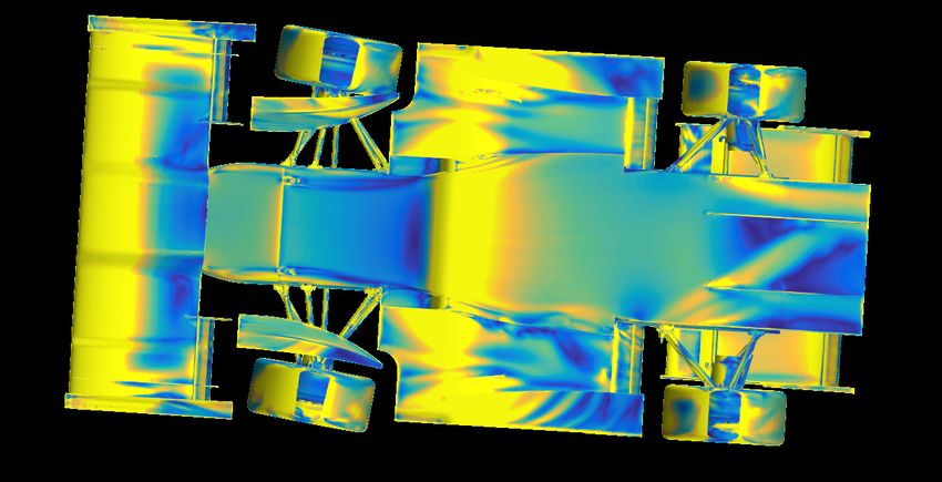
4.7 Skin friction coefficient on the car surface seen from below. . . . . . . 38
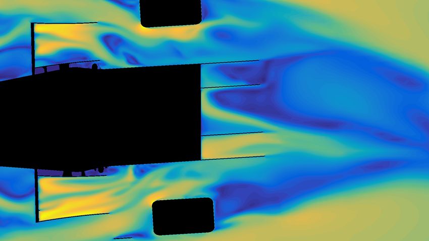
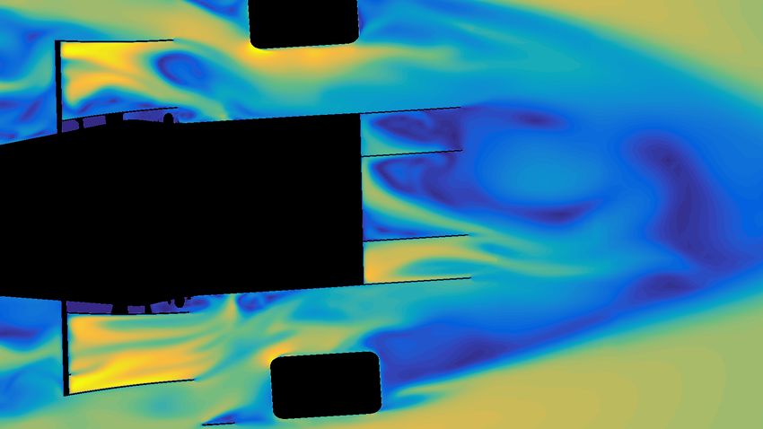
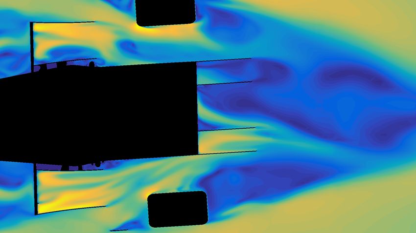
4.8 Vorticity magnitude for driving straight, braking and cornering. The
visualized yz-plane is cutting through the diffuser 230 mm behind the
monocoque. . . . . . . . . . . . . . . . . . . . . . . . . . . . . . . . . 40
4.9 Skin friction for different diffuser starting points while driving straight
and during cornering. . . . . . . . . . . . . . . . . . . . . . . . . . . . 42
4.10 Skin friction while driving straight for diffusers with different angles. . 44
4.11 Skin friction while cornering for diffusers with different expansion
angles. Note the differences in Venturi vortex generation between the
different cases. . . . . . . . . . . . . . . . . . . . . . . . . . . . . . . . 45
4.12 Difference in accumulated lift coefficient CL , relative to the 19◦ dif-
fuser for the straight and curved driving scenarios. A higher CL im-
plies a greater downforce. . . . . . . . . . . . . . . . . . . . . . . . . . 46
4.13 Vorticity magnitude while driving straight for the 13◦ and 19◦ dif-
fusers with and without strakes. The visualized yz-plane cuts through
the diffuser 27 mm behind the monocoque. . . . . . . . . . . . . . . . 48
4.14 Pressure coefficient on the underside surface of the car while driving
straight. The four different diffuser designs with expansion angles 13◦
and 19◦ , with and without strakes, are presented. . . . . . . . . . . . 49
4.15 Vorticity magnitude while cornering for the four diffusers with 13◦
and 19◦ angles with and without strakes. The visualized yz-plane
cuts through the diffuser 27 mm behind the monocoque. . . . . . . . 50
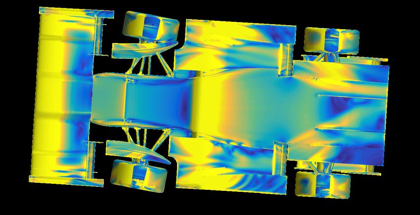
4.16 Skin friction on the underside of the car. The four different diffuser
designs with expansion angles 13◦ and 19◦ , with and without strakes,
are presented. . . . . . . . . . . . . . . . . . . . . . . . . . . . . . . . 51
xviList of Figures
4.17 Pressure coefficient for the 13° and 19° diffusers with and without side
floors while driving straight are illustrated. The visualized yz-plane
cuts through the diffuser 27 mm into the back of the monocoque. . . 52
4.18 Vorticity magnitude with and without side floors while driving straight.
The visualized yz-plane cuts through the diffuser 27 mm behind the
monocoque. . . . . . . . . . . . . . . . . . . . . . . . . . . . . . . . . 53
4.19 Velocity magnitude during cornering. The visualized xy-plane is lo-
cated at z = 78 mm above ground. . . . . . . . . . . . . . . . . . . . 54
4.20 Skin friction under the car with and without side floors while cornering. 55
A.1 Pressure coefficient under the car with and without side floors while
driving straight. . . . . . . . . . . . . . . . . . . . . . . . . . . . . . . II
xviiList of Figures xviii
List of Tables

3.1   The settings used in Star-CCM+. . . . . . . . . . . . . . . . . . . .        . 21
3.2   The boundaries for a straight simulation. . . . . . . . . . . . . . . .      . 23
3.3   The boundaries for a cornering simulation. For an accurate repre-
      sentation the system has to be viewed in a rotating reference frame.
      The reference frame contains the fluid volume and outer boundaries
      which rotates while the car is fixed. . . . . . . . . . . . . . . . . . .    . 24
3.4   Angles for simulating cornering at a corner radius of 12.5 m. For
      details regarding the different parameters, see Section 2.3. . . . . .       . 28

4.1   Values for CD , CL for different components and aero balance (rear-
      wards) for different driving scenarios using the small diffuser starting
      at the end of the monocoque. M&D stands for Monocoque & Diffuser,
      FW for Front Wing, RW for Rear Wing and SW for Side Wing. . .                . 29
4.2   Values for CD , CL , CL M&D and aero balance (rearwards) for the
      different diffuser starting points at the driving scenarios straight, cor-
      nering and braking. . . . . . . . . . . . . . . . . . . . . . . . . . . .    . 41
4.3   Values for CD , CL , CL M&D and aero balance (rearwards) for different
      diffuser expansion angles at the driving scenarios straight, cornering
      and braking. . . . . . . . . . . . . . . . . . . . . . . . . . . . . . . .   . 43
4.4   Values for CD , CL , CL M&D and Aero balance (rearwards) for 13◦
      and 19◦ diffusers with and without strakes. . . . . . . . . . . . . . .      . 47
4.5   Values for CD , CL , CL M&D and aero balance (rearwards) for 13°
      and 19° diffusers with and without side floors. . . . . . . . . . . . .      . 52
4.6   Values for CD , CL , CL M&D and aero balance (rearwards) for different
      driving scenarios comparing the small 0 mm diffuser and the best
      performing 13° diffuser with strakes and side floors. . . . . . . . . .      . 56

A.1 The side wings’ lift coefficient for all the straight simulations . . . . .       I
A.2 The side wings’ lift coefficient for all the cornering simulations . . . .        I

                                                                                    xix
List of Tables xx
1
                           Introduction

Formula Student (FS) is a competition where universities and engineering students
design and build formula cars. Chalmers team is called Chalmers Formula Student
(CFS) and has been building electric formula cars since 2015. The average speed
in competition for a Formula Student car is about 50 km/h, while the top speed
is about 110 km/h [1]. The current CFS car has a diffuser, but it is believed that
there is great potential in improving the flow around the floor and the diffuser to
create more downforce.

Downforce is a force that refers to the downward aerodynamic lifting force that
is obtained on a car when a pressure difference is created between the top and bot-
tom of the car. As downforce increases in a racing car, the tires generate more
friction, which results in increased grip against the ground. This means that the
car can accelerate more without the wheels spinning and that higher speeds can be
maintained in corners. A diffuser is an aerodynamic part belonging to the bodywork
at the rear of the car, see Figure 1.1. By applying a diffuser, the pressure under
the car can decrease in relation to the pressure above the car thus generating more
downforce. A diffuser also plays an important role in returning the air flow under
the car to the ambient air in a smooth way to minimize energy losses, reducing the
drag.

Figure 1.1: 3D representation of the CFS21 car. The diffuser is marked in red.

Different dynamic driving scenarios such as cornering, braking and acceleration af-
fect how well all the car’s aerodynamic components (aero package) work. The airflow
when the car is driving straight ahead at a constant speed does not interact with the
car in the same way as when the car is cornering. Thus, the pressure distribution

                                                                                   1
1. Introduction and consequently the downforce in the two cases differ. For a formula car, downforce is most critical in dynamic driving scenarios where the car’s grip is most important. Implementation of different dynamic driving scenarios in aerodynamic simulations has rarely been done by the CFS team. However, this is something the team believe will bring benefits for future aerodynamic development. A structured method for modeling of such dynamic scenarios would be favorable for the 2021/2022 CFS team (CFS22) and future CFS teams. 1.1 Historical Background Motorsport began developing in the end of the 19th century following the invention of the petrol fueled internal-combustion engine. Until 1960, the development of rac- ing cars consisted mainly of strengthening the engines and generating more grip by developing chassis and wheel suspension. This required costly investments, which led to only the largest manufacturers being able to afford continued development and thus the opportunity to fight for a top position during competition. For the smaller manufacturers, new cheaper development areas were therefore needed, and the development of aerodynamics came into focus. Previously, the development of car aerodynamics had been intended to reduce air resistance, but in the late 1960s, motorsport engineers observed that downforce was also important for faster corner- ing. This led to innovative designs of cars that used downforce, which resulted in drastically improved lap times. Since then, aerodynamics has played a central role in motorsports [2]. In Formula 1, in particular, aerodynamic improvements have been of great im- portance. With increased knowledge about aerodynamics, higher speeds can be maintained, but also lower fuel consumption, lower wind noise and higher comfort are achieved. In the late 60’s, the first F1 car with a front wing and a rear spoiler, the Lotus 49B, was presented. During this period experiments of having wings high above the body of the car were carried out on, for example, the Matra MS10. Since the 60’s, lots of technical innovations in aerodynamics have been tested. Among other things, skirts have been added to the body work, in order to get the maximum ground effect. Lots of different wing and underbody designs have also been tested [3]. One of the most radical F1 cars of all time was the Brabham BT46B, also known as the ”fan car”. The car was designed by Gordon Murray and was equipped with a large fan that generated an immense amount of downforce by extracting air from the underside of the car. The car only raced once at the Swedish Grand Prix in Anderstorp in 1978, where the car also won before the concept was withdrawn [4]. It is still an ongoing process for motorsport engineers to look for areas for aerodynamic improvement in order to find that little extra performance that is crucial in a race. 1.2 Objective The objective of this project is to develop a methodology for modeling of aerody- namic forces during different racing maneuvers of a CFS car. These new methods 2
1. Introduction

will then be used in the development of a new diffuser concept. This is done with the
aim of providing CFS with knowledge and proof-of-concept of the implementation
of a new diffuser, which could increase aerodynamic performance of the car.

1.3     Working Methods
The modeling of aerodynamic forces on the CFS car has been done using Computa-
tional Fluid Dynamics (CFD). Setups for relevant driving scenarios such as driving
straight ahead, cornering and braking were simulated using a range of new diffuser
design concepts. This was done in order to draw conclusions of how well a design
concept works in dynamic driving scenarios, i.e. how aerodynamically robust it is.

Design concepts were developed using 3D Computer Aided Design (CAD). A base
model of the CFS21 car was obtained from CFS and used as a baseline. Iterations
of a new diffuser concept were systematically developed and simulated using CFD.
Furthermore, CFS shared three post-processing scripts. These were edited and used
to produce necessary data and plots to analyze the simulations.

1.4     Delimitations
The project is delimited in several regards. For instance the diffuser concepts de-
veloped in the project will not be manufactured. It will only be visualized in three
dimensional CAD, and simulated using CFD.

When developing a new diffuser, the design is based on the rules for Formula Student
in 2022 [5]. However, the regulations tend to look different from year to year when
it comes to powered aero devices such as fans, which is the reason for the project
to develop a diffuser design that performs good even without fans. Should it be of
interest to add fans, then it should be for the purpose of tuning an already good
performance. Hence the project is based on a diffuser without fans.

In an aerodynamic package of a formula car, the aerodynamic components inter-
acts in complex and often unpredictable ways with each other. Because of this
complexity and the project’s limited time and computational resources, it is neces-
sary to have practical limitation of how in-depth the work can be. Therefore, the
design development will only be focused on the diffuser. Design of other parts of
the car’s aero package will thus not be covered in this project.

The project also does not include any mesh study. Mesh studies aim, among other
things, to ensure convergence and independence of mesh for the solution in the sim-
ulation. Instead of doing a mesh study, CFS current mesh was used with some
refinements since CFS has already performed one [6]. More about the refinements
are mentioned in Section 3.2.

Only CFD simulations will be performed in order to analyze the aerodynamics of

                                                                                   3
1. Introduction the formula car, an thus no wind tunnel experiments. Due to the fact that no wind tunnel experiments will be carried out, no validation will be made in the form of correlation between simulations in CFD and wind tunnel testing. This will not be possible due to, among other things, that no diffuser will be manufactured. Wind tunnel experiments are also resource and time consuming. Assumptions of stationary flow is made for all simulations in the project. This means that the car’s position and quantities, such as velocity and pressure, don’t change with time. This assumption is done due to the fact that non-stationary flow would be too time consuming to base the simulations on. Thermodynamic effects on the flow are not taken into account in the project either. This is because its impact is considered to have a relatively insignificant impact on this project. The project will primarily focus on generating as high downforce as possible. Drag force is of secondary priority. Downforce always comes with the penalty of increased dragforce. However, in Formula Student it has been shown that increased downforce results in faster lap times almost regardless of any realistic drag force penalty [7]. This is true up to a factor of ∆CD /∆CL = 3, where ∆CD is a unit of gained drag coefficient (see Section 2.1.2.2) and ∆CL a unit of gained lift coefficient (see Section 2.1.2.3), as shown by previous CFS team members. No major consideration is given to the packaging of electronic components when designing the diffuser. When testing how early a diffuser concept can begin, parts of the electronics and battery storage are cut off. However, a plausibility assessment is made in order to decide how much of the electronics can be moved in order to let the diffuser start earlier. 4
2
                                  Theory

In this chapter, the fundamental physics phenomena which are central to the project
are described. Further, the working principles of an undertray diffuser are investi-
gated.

2.1      Fundamental Fluid Dynamics Theory
The relevant portion of fundamental fluid dynamics theory is presented in this sec-
tion. These principles are relevant to describe aerodynamics as a subject. In addi-
tion, most of them are utilized by the CFD program Star-CCM+ which is further
described in Section 3.2. The presented variables are described in Nomenclature.

2.1.1     Bernoulli’s Principle and the Continuity Equation
In incompressible isentropic flow, i.e. a flow where a negligible amount of energy
is lost to non-reversible processes such as heat in turbulent flows, one can derive
Bernoulli’s principle from the conservation of energy

                              u2 p
                                + + z · g = constant,                              (2.1)
                              2  ρ
where z is the vertical position of a fluid element. This law states that an increase in
velocity implies a decrease in pressure and vice versa. This is the working principle
for wing profiles and diffusers [8].

Further, the continuity equation for mass flow provides a relationship between flow
area in a closed channel and flow velocity
                  ∂ρ                              ṁ
                     + ρ∇ · ~u = 0 =⇒ Aflow · u =    = constant,                   (2.2)
                  ∂t                              ρ
where Aflow represents the swept area of the fluid flow, t time and ṁ the mass flow
rate through Aflow .

2.1.2     Dimensionless parameters
Dimensionless parameters are used to make a parameter comparable with parame-
ters of other types of flow. Below the relevant parameters are presented.

                                                                                      5
2. Theory
2.1.2.1 Reynolds Number
The Reynolds number, Re, is a dimensionless number which tells the relation be-
tween the inertia and viscosity in a newtonian fluid and is defined as
( )
ρV L Inertia
Re = = (2.3)
µ Viscosity
V and L are the characteristic velocity and length of the flow. A high Re is associated
with a fast, large-scale turbulent flow, whereas a low Re corresponds to a slow,
viscous flow. Fast flows of gas imply a relatively high Re [8].
2.1.2.2 Drag Coefficient, CD
The drag coefficient of a body, CD , is a dimensionless number indicative of drag
force. CD is defined as
FD
CD = 1 2 , (2.4)
2
ρu∞ A
where A is the projected area from the front of the body and the denominator
( 21 ρu2∞ ) is the dynamic pressure of the free stream [8].
2.1.2.3 Lift Coefficient, CL
The lift coefficient of a body, CL is defined as
FL
CL = 1 , (2.5)
2
ρu2∞ A
where A is projected area from the front of the body. CL is a dimensionless coefficient
that increases with lift force [8]. In this study, CL will indicate the lift in negative
ẑ-direction, i.e. a high downforce will correspond to a large CL .
2.1.2.4 Pressure Coefficient, Cp
The pressure coefficient , Cp , is a dimensionless parameter that describes the relative
pressure. Cp is defined as
p − p∞
Cp = 1 , (2.6)
2
ρu2∞
where p is the static pressure at the point where Cp is calculated, while p∞ is the
static pressure in the free stream [8].
2.1.2.5 Skin Friction Coefficient, Cf
The skin friction coefficient, Cf , is a dimensionless parameter defined as [8]
τw
Cf = 1 . (2.7)
2
ρu2∞
62. Theory
2.1.3 Vorticity
~ is defined as the curl of the velocity field, ∇ × ~u, which relates to
The vorticity, ζ,
the rotation of a velocity field. If the vorticity is zero the flow has no rotation and
is called irrotational [8]. The voriticity in x direction is given by
∂w ∂v
ζx = − . (2.8)
∂y ∂z
2.1.4 Navier-Stokes Equations
A fluid can be described with the Navier-Stokes equations if it is incompressible and
newtonian [8] as !
∂~u
ρ + (~u · ∇)~u = ρ~g − ∇p + µ∆~u. (2.9)
∂t
2.1.5 RANS
In turbulent flow there are fluctuations that causes rapid changes in the velocity and
pressure in the Navier-stokes equations (Eq. 2.9). These rapid changes can be easier
to account for if the velocity and pressure are split into a mean variable ū and a
fluctuation variable u0 . The velocity in the x-direction is therefore u = ū+u0 . If those
splits is put into the Navier-stokes equations we get the Reynold’s Averaged Navier
Stokes (RANS) equations after some derivations [8]. The RANS in x-direction is
! ! !
du ∂p ∂ ∂u ∂ ∂u ∂ ∂u
ρ =− + ρgx + µ − ρu02 + µ − ρu0 v 0 + µ − ρu0 w0 .
dt ∂x ∂x ∂x ∂y ∂y ∂z ∂z
(2.10)
2.1.6 Flow Past Boundary
Bodies, such as plates, immersed in a fluid stream create a boundary layer flow.
The boundary layer is defined as the region where the flow velocity is less than 99
percent of the velocity of the external flow (u∞ ). The boundary layer flow is made
up of two parts, the laminar part and the turbulent part:
5
103 < Rex < 106 laminar flow
Re1/2
δ
x
≈ . (2.11)
x 0.16 6
10 < Rex turbulent flow
Re1/7
x
δ is the thickness of the boundary layer and Rex the Reynolds number at x [8]. An
illustration of he boundary level flow can be seen in Figure 2.1.
2.1.6.1 Flow Separation
Backflow, i.e. flow going in the opposite direction of the freestream, at the wall
indicates that the flow is separated. The point of separation is when the wall shear
is 0 which means the velocity gradient is 0 [8].
72. Theory
y
6 δ(x)
u∞
- -
- -
- - u(x, y)
- -
- -
Laminar part Turbulent part
-
Z
ZZZZ
ZZZZ
ZZZZ
ZZZZ
ZZZZ
ZZZZ
ZZZZ
ZZZZ
ZZZZ
ZZZZ
ZZZZ
ZZZZ
Z
- x
Figure 2.1: Flow close to a wall. The flow enters and acts laminar and then
changes and becomes turbulent at Rex > 106 .
2.1.6.2 The Logarithmic Overlap Law
The turbulent flow near a wall can be broken up in three regions based on which
shear stress dominates:
• Wall layer: Viscous shear dominates.
• Outer layer: Turbulent shear dominates.
• Overlap layer: A mix of the shear types.
We define the dimensionless number y + as
+yu∗
y = , (2.12)
ν
q
where u∗ = τw /ρ. For y + ∈ [0, 5] the inner layer dominates and is proportional to
y + . It can be described with the dimensionless variable
u
u+ = = y+. (2.13)
u∗
For y + ∈ [30, 103 ] the overlap layers dominates and can be described as
1
u+ = ln y + + B, (2.14)
κ
where κ ≈ 0.41 and B ≈ 5.0. For y + ∈ [5, 30] the inner layer has to curve so
it merges with the overlap layer. Only experimental data exists for this interval
making it difficult to model [8].
82. Theory
2.2 CFD Theory
Numerically solving the equations that describe the airflow around the car is a
complex process. It is important to determine the accuracy needed in the simulation
to arrive at a balance of the resources needed for the simulation and its accuracy.
Different mathematical models for the modeling of the flow can be used. These
models have their respective strengths and weaknesses, and should be chosen with
care. This requires a basic understanding of key concepts in CFD simulation.
2.2.1 Finite Volume Method
The Finite Volume Method (FVM) is a numerical method used to solve the partial
differential equations encountered in fluid mechanics. The first step in the FVM is
to discretize the domain of interest into a finite amount of control volumes (cells).
The variables of interest are located at the centroid of these cells. The second step
is integration of the governing equations over the cell to solve for these variables.
Lastly, interpolation profiles are assumed between cell centroids in order to describe
the variation of the variables of interest [9].
2.2.2 The k − Turbulence Model
k − is a type of RANS turbulence model that can be used in CFD. The k − model
solves the equations for k and where k is the turbulent kinetic energy and the
rate of dissipation. k − is accurate around external flow problems but not very
accurate in complex curves. The model is fast and has a good convergence rate [10].
2.2.3 The k − ω Turbulence Model
k − ω is likewise the k − model a type of RANS turbulence model . The k − ω
model solves the equations for k and ω where k is the turbulent kinetic energy and
ω is the specific dissipation rate. Contrary to the k − method, the k − ω method
is especially accurate in internal flow, flow past complex curvature and in separated
flow. The method is more complex than the k − model which leads to it being
slower and more difficult to converge [10].
2.2.4 The SST k − ω Model
The SST k−ω model is a mixup of the k−ω method and the k− method where SST
is Shear Stress Transport. Since the k − ω method is better near walls it influences
the result near the walls and because it’s not very good in the free stream there is
a transition from the k − ω method to the k − method in the free stream [11].
2.3 Vehicle Dynamics Theory
In this section, vehicle dynamics parameters relevant to this study are described.
Furthermore, aerodynamic influence on vehicle dynamics in relation to these param-
92. Theory
eters are discussed in this section.
2.3.1 Steering Angle
The steering angle is the angle between the direction of a wheel and the car’s longi-
tudinal axis. The steering angle for each front wheel can be different if the car has
Ackermann steering [12]. An illustration can be found in Figure 2.2.
δf l
δf r
Figure 2.2: Steering angles, δf l for the left wheel and δf r for the right wheel. These
angles can differ from each other if the car has Ackermann steering.
2.3.2 Body Slip Angle
The body slip angle is an yaw angle meaning it is the angle that is created when
the car rotates around its vertical axis. The rotational axis goes through the car’s
center of gravity. The body slip angle is the angle between the velocity vector of
the car and the car’s longitudinal direction [12]. A visual representation of the body
slip angle can be seen in Figure 2.3.
102. Theory
y
β
ac
x
β
~v
Figure 2.3: A body slip angle β. The car’s longitudinal direction is pointing in
the x direction while it is moving in a different direction ~v thus creating a slip angle
β. The centripetal acceleration ac is acting on the car’s center of mass towards the
corner’s center.
2.3.3 Pitch Angle
The pitch angle is the angle that is created if the vehicle’s sprung mass (everything
but the wheels) rotates around its lateral axis which is shown in Figure 2.4. The
vehicle rotates around what is called its pitch center [12].
θ
Figure 2.4: A pitch angle θ around the car’s lateral axis.
2.3.4 Roll Angle
The roll angle is the angle that is created if the vehicle’s sprung mass rotates around
its longitudinal axis, see Figure 2.5. The vehicle rotates around what is called its
roll center [12].
112. Theory
φ
Figure 2.5: A roll angle φ around the car’s longitudinal axis.
2.3.5 Ride Height
The ride height is the smallest distance between the ground and the car’s floor when
it is stationary, see Figure 2.6. For a Formula Student car the ride height must at
least be 30 mm [5].
Hr
Figure 2.6: A ride height Hr .
2.3.6 Aerodynamic Influence on Vehicle Dynamics
Vehicle dynamics is a large and complex subject. Mass distribution, tires, suspen-
sion setup and aerodynamics are examples of areas that greatly affect the dynamics
of a car. Basic principles of aerodynamics influence, in particular on a Formula
student car, is further discussed here.
The main aim of aerodynamics on a Formula Student car is to increase its negative
lift force (downforce). Greater downforce makes it possible for the tires to produce
larger forces (grip) while accelerating/braking (longitudinal forces) and cornering
(lateral forces). The basic formula describing this relationship is Flong/lat = Fz µ,
where Flong/lat is the longitudinal or latitudinal force, Fz the normal force which
is increased with increased downforce and µ the friction coefficient. Consequently,
the speed of the car can be increased in most driving scenarios or the same grip
can be achieved with less tire slip, i.e smaller slip angle, when compared to a car
with less downforce. This helps reducing heat production and therefore preserve tire
life. Furthermore, smaller slip angles are easier to control for the driver. The car’s
stability in this case is improved compared to larger slip angles and aerodynamic
parts tend to work more efficiently, improving the balance [3].
In most cases a weight and aerodynamic distribution close to 50/50 on the cars
122. Theory
rear and front axle is desired. A car with the center of gravity (COG) closer to the
front axle usually generates more understeer. Conversly the aerodynamic center of
pressure (COP or aero balance), the point at which the resultant downforce is lo-
cated, closer to the front usually generates more oversteer. A car with a front biased
COG can therefore be counter balanced by placing the COP forwards. However, it
is favourable in some cases, in CFS’s case for example, to design the aerodynamic
package with a COP slightly rear biased. This can generate understeer, but under-
steer is considered more stable and easier to control when compared to oversteer [3].
Vehicle dynamics parameters described in previous sections are closely related to the
aerodynamic package on a given car. While the generated downforce affect body
slip, pitch and roll angles, these parameters in turn affect the aerodynamic efficiency.
Pitch angles for example can have a large impact on vehicle balance. When braking
and pitching forwards, the front wing’s downforce is generally increased. Although,
other factors such as already low static ride height or an extreme pitch angle might
cause a decrease in downforce for the front wing. This also results in less air flow to
the car’s floor and diffuser, decreasing the middle and rear downforce. If the front
wing downforce increases, the aerodynamic balance shifts forwards, decreasing the
stability of the car. While this is considered unfavourable, increased grip on the front
axle also results in improved braking capabilities. On the contrary, if the downforce
on the front wing decreases the balance shifts rearwards and the opposite occurs.
It is more difficult to describe the influence of steering and roll angles. These affect
the aerodynamics in an asymmetric manner and can cause unpredictable behaviour
of the car. The same is true for body slip angles, or yaw angles, where the air flow
hits the car with an angle from the longitudinal axis [3].
A diffuser expands the airflow underneath the car’s floor. This expansion forces
the flow upstream to increase in speed in order to fill up the larger volume in the
diffuser, decreasing the pressure upstream. In motorsport it has been observed that
diffusers are particularly effective aero devices. The reason is that diffusers increase
the vehicle’s downforce under the whole floor. Downforce in this region is close to
the center of the car and distributed over a large aera. This results in good balance
contribution and makes the vehicle less sensitive to pitch or other phenomena that
affect the balance. In order for a diffuser to work efficiently, the front wing needs
to supply the floor and diffuser area with sufficient airflow. Optimally the airflow’s
velocity is large and laminar. Another option for increasing the airflow is by feeding
the diffuser with air from the sides of the vehicle. This can however interfere with
the low pressure diffuser region and increase the pressure, resulting in a decrease
of downforce. A compromise between keeping the floor sealed and increasing the
airflow is usually optimal. This airflow can also be used to induce vortices, as
described in the next section [3].
2.4 Working Principles of a Race Car Diffuser
The main function of an undertray diffuser is to reduce the pressure upstream of the
diffuser, which provides a greater amount of downforce. Additionally, the diffuser
132. Theory
provides a smooth transition where the airflow under the car joins the wake region.
Equation (2.1) and Equation (2.2), can be combined to relate pressure, flow velocity
and the area swept by the flow (i.e. the space between the car and the ground):
1 ṁ 2 p
+ = constant, (2.15)
2 ρAflow ρ
Where the parameters are as in the previously mentioned equations. It is clear that
a decrease in flow area promotes a decrease in pressure. Given the boundary con-
dition of ambient pressure at the end of the diffuser, one can see that the diffuser
promotes a negative pressure upstream, providing downforce.
However, this simplified model describes the undertray diffuser as a closed tube, in
which the flow is perfectly laminar. A more accurate model would account for the
air introduced from the gap between the diffuser sidewalls and the road as well as
energy lost to complex, turbulent flow.
2.4.1 Effect of Different Design Parameters of the Diffuser
The geometry of a simple race car diffuser can be described by a number of key design
parameters. These all have their respective effects on the airflow, and interact in
complex ways.
2.4.1.1 Differences in the Angles of the Diffuser
The maximum angle of the diffuser channel’s upper boundary relative to the xy-
plane is referred to as the expansion angle of the diffuser. This angle determines
to a great extent how well the flow attaches. A typical value is around 15°. A
substantially higher angle will result in separation of the flow from the inside of the
diffuser, resulting in an increase in pressure [13].
2.4.1.2 Differences in Area Ratio
The area ratio of a diffuser is related to the angle of the diffuser and the length of
the diffuser volume by simple geometry.
Hr + Ld · sin(θ) Ainit
flow
Rar = = final , (2.16)
Hr Aflow
where Rar denotes the area ratio, θ the angle of the diffuser, Hr the ride height,
Ainit final
flow the inlet area of the diffuser, Aflow the rear outlet area of the diffuser, and Ld
the length of the diffuser volume.
Combining this equation with Equation (2.15) makes it clear that lower pressures
can be obtained with longer diffusers and larger diffuser angles. However, a practical
limit is reached when the area ratio approaches 1:5. At this point, the high pressure
ambient air starts to interfere with and spoil the airflow, decreasing downforce [13].
142. Theory
2.4.1.3 Implementation of Strakes
Vertical panels in the diffuser volume, with the purpose of directing the airflow are
referred to as strakes. Strakes lower the characteristic length of the flow, keeping
the latter laminar and lowering the pressure. Other effects can be promoted by
directing the airflow in different ways [3].
2.4.1.4 Different Throats of the Diffuser
The throat or kick of the diffuser is where the underfloor transitions to the diffuser
ramp surface. The lowest pressure in the airstream is located in the throat, meaning
that this area provides a non-negligible amount of downforce. The radius of this
throat determines to some extent how the flow behaves inside the diffuser. A small
radius will make the flow prone to separation downstream of the throat, but may
also increase downforce by increasing underbody area [8].
2.4.2 Venturi Vortices
The performance of the diffuser is highly dependent on that the flow remains at-
tached to the internal surface of the diffuser. As discussed, this stands in contrast
to the measures taken to decrease pressure in and upstream of the diffuser. To keep
the flow from separating, a vortex pair can be induced. The flow in such vorticies
have a short characteristic length, and stay laminar to a greater degree. Methods
to induce the desired vortices include:
• Direction of airflow over a sharp edge, such as over the diffuser sidewall
• Implementation of turning vanes, i.e. small winglets upstream of the diffuser,
which give the flow closest to the car surface sideways momentum
• Implementing strakes in the diffuser channel, which contain and keep the vor-
tices undisturbed.
Figure 2.7: 3D-schematic showing the typical vortex pair that form as high-
pressure ambient air flows into the low-pressure cavity of the undertray diffuser
(red arrows). Note the direction of the vortex rotation. The blue streamlines are
grossly simplified.
To some extent, the vortices also keep the high-pressure outside separated from the
152. Theory low-pressure inside of the diffuser. This effect decreases pressure upstream of the diffuser, thus increasing aerodynamic performance [3]. 16
3
                               Methods

The methods used in the project are presented in detail in this section. The workflow
for creating and simulating a diffuser is shown in Figure 3.1.

      Pre Processing
                                   Simulation                Post Processing
      • CAD design
                                  • Boundary con-            • Post script
      • Modeling of
                                    ditions                  • Calculation of
        driving scenar-
                                  • Physics models              coefficients
        ios
                                  • Convergence              • Figures of flow
      • Surface prepa-
                                    conditions                  quantities
        ration and mesh

Figure 3.1: Workflow for the development of a diffuser.

3.1     CAD
To enable simulations of the Formula Student car a 3D-model was required. CAD
was used to design all the geometries of the aerodynamics package before it was
imported and pre-processed in the CFD software Star-CCM+. In order to create
these CAD models, the software Catia V5 was used. The project was provided with
the CAD model of the CFS21 car, i.e. the latest model, from which the design work
could be based upon. The aerodynamic parts of the CFS car are shown in Figure 3.2.
Since the project aims to study how a new diffuser could increase the performance
of the formula car, all parts that were not connected to the diffuser could remain
the same. Overall, only the diffuser and the monocoque were affected (in terms of
direct contact) by the diffuser replacement. The monocoque is the self-supporting
chassis of the car, which can be visualized in grey in Figure 3.2.

                                                                                  17
3. Methods Figure 3.2: CAD model with the aerodynamic parts marked in different colors. Front wing (orange), deflector (red), monocoque (grey), side wing (green), rear wing (blue) and diffuser (yellow). 3.1.1 Current diffuser As a starting point, a simplified version of CFS’s latest diffuser was used. However, the current diffuser features an aggressive diffuser expansion angle which makes it difficult for the flow to remain attached. CFS21 has solved this by integrating the cooling package on the diffuser, and thus creating a suction normal to the flow di- rection. This results in a higher extraction of air and thus a higher downforce. The CFS21 diffuser is shown in Figure 1.1. 3.1.2 Design Methodology To create a aerodynamically robust and well performing diffuser a number of design iterations were made. The design methodology was based on a number of basic concepts. The concepts includes the effect of how early on the monocoque the diffuser can start as well as the the expansion angle of the diffuser. After these concepts had been tested and evaluated, more detailed components were added. These components were strakes and side floors. As previously mentioned, the basic ideas of CFS’s current diffuser were used as a starting point in the design development. Therefore, the first diffuser simulated had the same monocoque as CFS21. In order to start the design iterations with a basic geometry both side floors and strakes were not included. For the remaining design iterations it was chosen to redesign the monocoque. In that way, the diffuser could start earlier on the underside of the car, thus making the expansion of air more prolonged. It is considered an interesting aspect to study in order to find out if the downforce would increase. 18
3. Methods

The starting point of the diffuser, i.e how far from the back of the monocoque the
diffuser starts, was iterated. The two extreme cases of starting the diffuser as early
as possible (500 mm in front of the monocoque rear wall) and as late as possible
(coinciding with the monocoque rear wall) were tested. An alternative concept be-
tween the extreme cases was also tested, where the diffuser instead started 300 mm
in to the monocoque. All three designs are displayed in Figure 3.3. The 300 mm
design was similar to the 500 mm case. Their difference being that the 300 mm
starting point resulted in a smaller throat radius connecting the flat underfloor and
the diffuser’s final angle of 15°. It was then possible to draw conclusions regarding
which design showed the most potential and attachment of flow.

Figure 3.3: Outlines of the three different diffuser designs when iterating the
starting point of the diffuser. The 500 mm design is displayed as purple, the 300
mm design as red and the 0 mm design as blue.

The angle between the flat bottom of the monocoque and the top of the diffuser
was also iterated. The angles tested were 13°, 15°, 17° and 19° which are displayed
in Figure 3.4. The project group chose to test four different angles due to time lim-
itations, especially in terms of simulation time. 15° was estimated to be the angle
corresponding to a reasonable movement of electronics in the rear of the current CFS
car. The other three angles were chosen at a linear scale to see how both slightly
higher and lower angles affect the diffuser.

Figure 3.4: Outlines of the four different diffuser designs when iterating the angle
between the flat bottom of the monocoque and the top of the diffuser. The 13°
design i displayed as blue, the 15° design as purple, the 17° design as red and the
19° design as green.

                                                                                   19
3. Methods After these basic design concepts had been tested, strakes and side floors were added to the designs that had performed best so far. The idea behind adding strakes was to induce more vortices and the idea behind side floors was to enlarge the low pressure surface of the diffuser, both adding downforce. Strakes were added by copying the outer walls of the diffuser and placing the copies at a fourth of the diffuser’s width symmetrically around the middle line. The side floors were designed with the same width as the current CFS car’s side floors. See Figure 3.5 for details. Figure 3.5: Diffuser with both strakes (orange) and side floor (blue). 3.2 CFD As computer performance has increased over the recent decades, computational fluid dynamics have become a more powerful tool. This section contains the setup for the simulations. 3.2.1 Whole-car Versus Half-car Symmetry Simulation Previous CFS teams have mostly used a half-car symmetry model for the simulations in the design process. The near-symmetric geometry of a car was exploited to decrease the computational resources needed. This resulted in less computing time and more simulations. However, due to the asymmetric flow during cornering, a half-car symmetry simulation is not possible for all scenarios. Previous CFS teams have also noted discrepancies between the two simulation models’ results. This might be due to small asymmetries between the car’s left and right features and geometry. Another cause might be that the symmetry plane boundary conditions of the half-car symmetry simulation are over-simplified. To ensure comparable results for the different simulated scenarios, it was decided to only do whole-car simulations. This trade-off increases simulation run time, but provides greater confidence in the simulation results. 3.2.2 Physics Model All the physics models were taken from CFS’s previous simulations, and can be seen i Table 3.1. Star-CCM+ is set to use SST k − ω turbulence modeling because it 20
You can also read