Technical Note: Flow velocity and discharge measurement in rivers using terrestrial and unmanned-aerial-vehicle imagery - Hydrol-earth-syst-sci.net
←
→
Page content transcription
If your browser does not render page correctly, please read the page content below
Hydrol. Earth Syst. Sci., 24, 1429–1445, 2020
https://doi.org/10.5194/hess-24-1429-2020
© Author(s) 2020. This work is distributed under
the Creative Commons Attribution 4.0 License.

Technical Note: Flow velocity and discharge measurement in rivers
using terrestrial and unmanned-aerial-vehicle imagery
Anette Eltner1 , Hannes Sardemann1 , and Jens Grundmann2
1 Institute   of Photogrammetry and Remote Sensing, Technische Universität Dresden, Dresden, 01069, Germany
2 Institute   of Hydrology and Meteorology, Technische Universität Dresden, Dresden, 01069, Germany

Correspondence: Anette Eltner (anette.eltner@tu-dresden.de)

Received: 6 June 2019 – Discussion started: 25 June 2019
Revised: 17 January 2020 – Accepted: 17 February 2020 – Published: 27 March 2020

Abstract. An automatic workflow to measure surface flow           1   Introduction
velocities in rivers is introduced, including a Python tool.
The method is based on particle-tracking velocimetry (PTV)
and comprises an automatic definition of the search area for      Measuring the discharge of rivers is a major task in hydrom-
particles to track. Tracking is performed in the original im-     etry because of its importance in many hydrological and ge-
ages. Only the final tracks are geo-referenced, intersecting      omorphological research questions, e.g. to understand the
the image observations with water surface in object space.        characteristics of catchments and their adaption to climatic
Detected particles and corresponding feature tracks are fil-      changes. Different approaches exist to apply the velocity–
tered considering particle and flow characteristics to miti-      area method to measure discharge relying on information
gate the impact of sun glare and outliers. The method can         about the flow velocity and the wetted river cross-section
be applied to different perspectives, including terrestrial and   area. Established tools to retrieve flow velocities are the ap-
aerial (i.e. unmanned-aerial-vehicle; UAV) imagery. To ac-        plication of current meters, acoustic devices (i.e. acoustic
count for camera movements images can be co-registered in         Doppler current profilers; ADCPs) or surface velocity radar
an automatic approach. In addition to velocity estimates, dis-    (Herschy, 2008; Merz, 2010; Morgenschweis, 2010; Grav-
charge is calculated using the surface velocities and wetted      elle, 2015; Welber et al., 2016). However, these velocity es-
cross section derived from surface models computed with           timation methods are either labour intensive, require mini-
structure-from-motion (SfM) and multi-media photogram-            mum water depths, need prolonged measurement periods or
metry. The workflow is tested at two river reaches (paved         can endanger the operator during flood measurements.
and natural) in Germany. Reference data are provided by              A promising alternative is remote sensing tools utilising
acoustic Doppler current profiler (ADCP) measurements. At         image-based approaches. Due to their flexibility (only a cam-
the paved river reach, the highest deviations of flow velocity    era is needed) they are used frequently exploiting various
and discharge reach 4 % and 5 %, respectively. At the natural     sensors and platforms for data acquisition. For instance, RGB
river highest deviations are larger (up to 31 %) due to the ir-   (red–green–blue) sensors have been used (e.g. Muste et al.,
regular cross-section shapes hindering the accurate contrast-     2008) as well as thermal cameras (e.g. Puleo et al., 2012).
ing of ADCP- and image-based results. The provided tool           Ran et al. (2016) demonstrated the suitability of a low-cost
enables the measurement of surface flow velocities indepen-       Raspberry Pi camera to observe flash floods, and Le Coz et
dently of the perspective from which images are acquired.         al. (2016) and Guillén et al. (2017) illustrated the usability
With the contactless measurement, spatially distributed ve-       of crowd-sourced imagery for post-flood analysis. Image-
locity fields can be estimated and river discharge in previ-      based setups allow for the assessment of temporally changing
ously ungauged and unmeasured regions can be calculated,          flow dynamics (Sidorchuk et al., 2008) due to the potential
solely requiring some scaling information.                        continuous recording of entire river reaches. Furthermore,
                                                                  small-scale investigations are enabled as shown by Legout et
                                                                  al. (2012), who measured the spatial distribution of surface

Published by Copernicus Publications on behalf of the European Geosciences Union.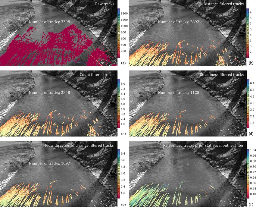
1430                                                       A. Eltner et al.: Flow velocity and discharge measurement in rivers

runoff from depths of millimetres to centimetres, at a range         cient is assumed to be (Le Coz et al., 2010). The coefficient
where other methods are failing.                                     can vary with different river cross sections (Le Coz et al.,
   Various algorithms exist for surface flow velocity monitor-       2010), and it can change within the same cross section due
ing from image-based observations deploying tracking tools.          to varying water depths, which is likely for irregular profiles
Four tracking approaches are applied frequently in the field         (Gunawan et al., 2012). Muste et al. (2008) state that the co-
to monitor rivers. The first method is large-scale particle im-      efficient mostly ranges between 0.79 to 0.93, but values as
age velocimetry (LSPIV) originally introduced by Fujita et           low as 0.55 have been measured (Genç et al., 2015). Consid-
al. (1998). This approach uses the tracking of features at the       ering the correct velocity coefficient is important because it
water surface that are caused due to natural occurring float-        has a high impact on the discharge estimation error in remote
ing particles or free surface deformations caused by ripples         sensing approaches (Dramais et al., 2011).
or waves, e.g. due to wind or turbulence (Muste et al., 2008).          When flow velocities and the velocity coefficient are
In general, the area of interest (i.e. the water surface) is di-     known, the area of the river cross section is needed to calcu-
vided in sub-regions, and these sub-regions are used as tem-         late the discharge with the velocity–area method (e.g. Hauet
plates. In the subsequent images, the corresponding areas are        et al., 2008). Different tools exist for contactless river area
searched for using correlation techniques.                           measurements of a cross section. Muste et al. (2014) show
   Fujita et al. (2007) advanced the LSPIV approach by an al-        that it is possible to use velocity pattern measured with
gorithm called space–time image velocimetry (STIV). STIV             LSPIV to retrieve flow depth in shallow-flow conditions. An-
performs faster because tracking is performed in 1D instead          other approach is the utilisation of ground-penetrating radar
of 2D. Profiles are extracted along the main flow direction to       as illustrated for larger rivers by Costa et al. (2000). An ad-
subsequently draw particle movements along the time axis             ditional increasingly used method to retrieve the topographic
(i.e. change along the profiles within succeeding frames),           (and thus cross-section) information of the river reach is the
leading to a space–time image. The resulting angle of the            usage of structure-from-motion (SfM) photogrammetry (Elt-
pattern within that image resolves into the flow velocity.           ner et al., 2016). For instance, Ran et al. (2016) capture
   The third possibility is the usage of optical flow algorithms     stereo images to reconstruct the 3D information of a river
developed in the computer vision community. For instance,            reach from overlapping images during low-flow conditions.
the Lucas–Kanade (Lucas and Kanade, 1981) operation has              However, if water is present during data acquisition and the
been utilised to measure surface velocities of large floods or       riverbed is still visible, the underwater measurements have
small rivers (Perks et al., 2016 or Lin et al., 2019, respec-        to be corrected for refraction impacts (Mulsow et al., 2018)
tively). The method aims to minimise greyscale value dif-            or else heights of points below the water surface will be un-
ferences between the template and search area adapting the           derestimated. Woodget et al. (2015) introduce a workflow to
parameters of an affine transformation within an optimisation        account for refraction using a constant correction value for
procedure. Finally, particle-tracking velocimetry (PTV) is a         the case of Nadir viewing image collection. Dietrich (2017)
tracking option that uses correlation techniques as in LSPIV.        extends this correction procedure for the case of oblique im-
However, instead of using entire sub-regions as templates,           agery. Detert et al. (2017) were the first to perform fully con-
single particles are detected first and then searched for in the     tactless, image-based discharge estimations using refraction
subsequent images.                                                   corrected river cross sections (adapting Woodget et al., 2015)
   LSPIV is the most widely used method and can be consid-           and surface flow velocities, all measured from unmanned-
ered as matured (Muste et al., 2011). Amongst other things, it       aerial-vehicle (UAV) imagery. However, the authors relied
enabled the measurement of the hysteresis phenomena dur-             on a seeded flow to apply LSPIV.
ing flood events (Tsubaki et al., 2011; Muste et al., 2011).            Image-based tracking approaches can be applied to im-
However, LSPIV mostly underestimates velocities, which is            agery captured terrestrially as well as from aerial platforms.
revealed in more detail by Tauro et al. (2017), who prefer           In the case of aerial imagery, the utilisation of UAVs for
PTV instead. In contrast to LSPIV PTV does not assume sim-           data acquisition is increasing. The advantage of drones is
ilar flow conditions for the entire search area, and it is not in-   their flexibility and allowance to capture runoff patterns
fluenced by surface frictional resistance (Lewis and Rhoads,         during high-flow conditions (e.g. Tauro et al., 2016; Perks
2015) or standing waves (Tsubaki et al., 2011).                      et al., 2016; Detert et al., 2017; Koutalakis et al., 2019),
   Besides surface flow velocity another parameter has to be         even enabling real-time data processing (Thumser et al.,
considered to derive discharge measurements from image-              2017). However, a challenge to overcome is the correction
based tracking approaches. The depth averaged flow velocity,         of camera movements during the UAV flight. Although cam-
used in the velocity–area method, does not necessarily cor-          era mounts are commonly stabilised, the remaining motion
respond to the surface flow velocity, which is amongst other         needs to be accounted for. Tauro et al. (2016) subtract veloci-
reasons due to the influence of riverbed roughness. There-           ties measured in stable areas outside the river from velocities
fore, a so-called velocity coefficient has to be used to ad-         tracked in the river. Another possibility is the usage of co-
just the surface velocities (Creutin et al., 2003; Le Coz et al.,    registration. Thereby, either features (e.g. scale invariant fea-
2010). Usually, the deeper the flow is, the higher the coeffi-       ture transform – SIFT – features; Lowe, 2004) are searched

Hydrol. Earth Syst. Sci., 24, 1429–1445, 2020                                      www.hydrol-earth-syst-sci.net/24/1429/2020/
A. Eltner et al.: Flow velocity and discharge measurement in rivers                                                               1431

for in stable areas (Fujita et al., 2015; Blois et al., 2016) or    2     Methods
ground control points (GCPs) are detected (Le Boursicaud
et al., 2016). Subsequently, these image points are matched         In this study, the FlowVelo tool is introduced that allows for
across the images. Afterwards, this information is used to ap-      the measurement of flow velocity from videos independently
ply a perspective transformation to each image to fit them to a     of the acquisition platform, i.e. either aerial or terrestrial. Dif-
reference image. However, so far stable areas are still masked      ferent parameter options for feature detection and tracking as
manually.                                                           well as track filtering are explained. Two experimental study
   In the case of terrestrial data acquisition, the conversion of   sites have been chosen to evaluate the performance of video-
pixel measurements to metric velocity values is more chal-          based flow velocity estimation using camera frames acquired
lenging compared to UAV data due to a stronger deviation of         from different perspectives. First the experimental study sites
the perspective from an orthogonal projection, which leads to       are introduced, and afterwards the tool is explained.
decreasing accuracies with increasing distance to the sensor.
Therefore, Kim et al. (2008) suggest to avoid camera setups         2.1     Areas of interest
with tilting angles larger than 10◦ . Most approaches ortho-
                                                                    The experimental study sites are short river reaches in Sax-
rectify the images prior to tracking to allow for a correct
                                                                    ony, Germany (Fig. 1). One studied river reach is situated
scaling of the image tracks. However, performing the track-
                                                                    at the Wesenitz. This river originates in the Lausitzer high-
ing in the original image would be favoured to minimise in-
                                                                    lands, has a catchment size of about 280 km2 and exhibits
terpolation errors, especially for oblique camera setups, and
                                                                    a river length of 83 km. The area of interest is located at
to solely transform the tracked image point coordinates into
                                                                    the river gauge station Elbersdorf, which is operated by
object space (Stumpf et al., 2016).
                                                                    the Staatliche Betriebsgesellschaft für Umwelt und Land-
   Several software tools already exist to perform image-
                                                                    wirtschaft, the Saxon state company for the environment and
based velocimetry (e.g. PTVlab from Brevis et al., 2011;
                                                                    agriculture. Here, annual average water level and discharge
PIVlab from Thielicke and Stamhuis 2014; Fudaa-LSPIV
                                                                    for the hydrological year 2017 are 48 cm and 2.4 m3 s−1 , re-
at https://forge.irstea.fr/projects/fudaa-lspiv (last access:
                                                                    spectively. Field campaigns were conducted on 31 March
24 March 2020); KU-STIV developed by Fujita; Rectifica-
                                                                    and on 4 April 2017. During the campaigns, the water level
tion of Image Velocity Results – RIVeR – from Patalano
                                                                    amounted 51 cm (discharge 2.7 m3 s−1 ). The investigated
et al., 2017). These tools cover different processing steps
                                                                    river section at the Wesenitz is paved but influenced by local
and tracking options to retrieve surface flow velocities and
                                                                    sand banks at the river bottom. During the data acquisition
discharge. In this study, we combine the entire workflow
                                                                    the river had a width of about 10 m.
from video, either captured with a UAV or from a terrestrial
                                                                       The other river is the Freiberger Mulde, which origi-
camera, to the velocity of river reaches, considering image
                                                                    nates in the Ore Mountains, has a catchment size of about
stabilisation, automatic feature search area extraction, PTV,
                                                                    2980 km2 and displays a river length of 124 km. The area of
track filtering and metric velocity retrieval via forward ray
                                                                    interest is located close the gauge Nossen. Average discharge
intersection. An automatic flow velocity measurement tool
                                                                    and water level for the hydrological year 2016 are 5.6 m3 s−1
(FlowVelo tool) for image velocimetry is presented and pro-
                                                                    and 65 cm, respectively. The gauge station is located 1 km
vided to the public domain to overcome existing gaps dis-
                                                                    upstream of the studied river reach. The field campaign was
cussed before. It is independent from the data acquisition
                                                                    conducted on 26 October 2016. During this day discharge
scheme and relies on PTV. Camera movements are accounted
                                                                    and water level were 5.7 m3 s−1 and 68 cm. The approxi-
for in a fully automatic approach if a sufficient amount of
                                                                    mated river width was 15 m. The chosen region of interest
shore area is visible. Furthermore, the search area for features
                                                                    at the Freiberger Mulde is a natural river section with non-
to track, i.e. the river area, is extracted automatically solely
                                                                    uniform flow conditions.
requiring water level information and a 3D surface model
of the river reach. The 3D surface model is calculated from
                                                                    2.2     Data acquisition
image data with SfM photogrammetry additionally consid-
ering multi-media photogrammetry to retrieve both topogra-          Different data were collected during the field campaigns at
phy and bathymetry. In order to improve tracking results, de-       both river sections. Amongst other things, ADCP measure-
tected features and velocity tracks are filtered with different     ments were performed as a flow velocity reference; GCPs
methods. Finally, we estimate discharge from surface flow           were defined to geo-reference the video data; and UAV and
velocities and cross-sectional areas. The FlowVelo tool and         terrestrial imagery were acquired to perform image-based
the whole workflow are investigated for two river reaches,          flow velocity estimation.
paved and natural, at which velocities and discharges are
compared to ADCP references.                                        2.2.1    ADCP measurements

                                                                    For the ADCP measurements the moving boat approach with
                                                                    StreamPro from RDI is used. Velocity profiles were mea-

www.hydrol-earth-syst-sci.net/24/1429/2020/                                       Hydrol. Earth Syst. Sci., 24, 1429–1445, 2020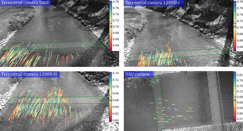
1432 A. Eltner et al.: Flow velocity and discharge measurement in rivers
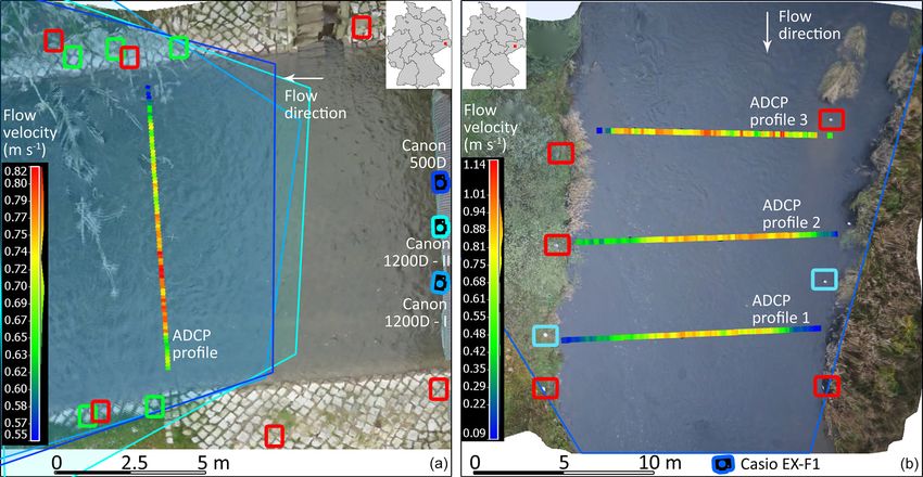
Figure 1. Areas of interest at the Wesenitz (a) and the Freiberger Mulde (b) displayed with UAV orthophotos calculated from video frames.
Surface flow velocities measured with an ADCP and the corresponding locations of the measurement cross sections within the river are
illustrated. Ground control points are used to reference the image data at both river reaches. Red squares highlight GCPs used for terrestrial
and UAV data at the Freiberger Mulde and UAV data at the Wesenitz. Green squares show the location of GCPs used for terrestrial imagery
at the Wesenitz. Check points (blue squares) are used to assess the accuracy of the 3D reconstruction from video frames at the Freiberger
Mulde. Camera locations of the terrestrial image sequence acquisition are illustrated as pictograms, and corresponding image extent areas
are shown (displayed area of interests in RGB correspond to the aerial image extents).
sured with a blanking range of 14 cm near the water sur- fore reveals a variation of about 4 %, which can be attributed
face. Data were processed using the AGILA software from to inconsistencies during data acquisition. A decrease of the
the German Federal Institute of Hydrology (BfG). Measure- velocity coefficient, which has been derived from the ADCP
ments along the boat track were projected onto a reference measurements, with decreasing water depth is observed. At
cross-sectional area. Afterwards surface flow velocities were the Freiberger Mulde, cross sections 1 and 3 (Table 1) have
extrapolated to allow for a comparison to the image-based lower water depth compared to profile 2. Thus, the velocity
values. For the extrapolation, power functions were fitted coefficients are lower.
to the measured vertical velocity profile for each individual
ADCP ensemble using the software AGILA (for more detail 2.2.2 Image-based data
see Adler, 1993, and Morgenschweis, 2010). Then, veloci-
ties at the water surface were calculated with these functions. At both river reaches video sequences were acquired with
Thus, all ADCP measurements of the profile were considered terrestrial cameras and with a camera installed on the UAV
to extrapolate surface velocities. AscTec Falcon 8. The airborne image data were captured
At the Wesenitz ADCP measurements were performed at at flying heights of about 20 and 30 m at the Wesenitz and
one cross section in eight repetitions (Fig. 1a). Average water Freiberger Mulde, respectively. Videos were captured with a
surface velocity was about 0.7 m s−1 , and the resulting dis- frame rate of 25 frames per second (fps) and with a resolu-
charge amounted to 2.7 m3 s−1 (Table 1). At the Freiberger tion of 1920 × 1080 pixels using the Sony NEX-5N camera
Mulde three cross sections were chosen (Fig. 1b) to acquire with a fixed lens with a focal length of 16 mm. The ground
data that allow for a spatially distributed assessment of the sampling distance (GSD) is about 7 mm at the Wesenitz and
image-based data. Average river surface velocities ranged be- about 9 mm at the Freiberger Mulde.
tween 0.60 and 0.76 m s−1 (Table 1). The terrestrial cameras were installed at bridges across the
The spatial variation of flow velocities is larger at the river (Fig. 1). At the Wesenitz three cameras were installed
Freiberger Mulde, where measurements were performed in to evaluate the performance of different cameras (Fig. 1a).
a natural river reach, which is in contrast to the flow ve- Two Canon EOS 1200D cameras and one Canon EOS 500D
locity range at the Wesenitz, where data were captured at a camera were set up. The 1200D cameras captured video se-
standardised gauge station. Thus, only one profile was mea- quences at 25 fps and with a resolution of 1920 × 1080 pix-
sured at the Wesenitz. The discharge at the Freiberger Mulde els. The 500D captured frames with a higher rate (30 fps)
is 5.88 m3 s−1 on average but reveals a standard deviation of and smaller image resolution (1280 × 720 pixels). All three
0.25 m3 s−1 . The estimated discharge of the river reach there- cameras were facing downstream. At the Freiberger Mulde
the Casio EX-F1 camera, equipped with a zoom lens fixed to
Hydrol. Earth Syst. Sci., 24, 1429–1445, 2020 www.hydrol-earth-syst-sci.net/24/1429/2020/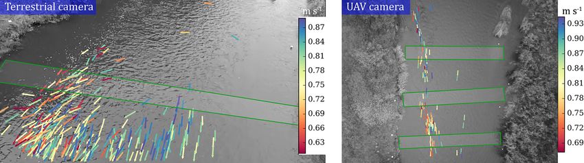
A. Eltner et al.: Flow velocity and discharge measurement in rivers                                                            1433

Table 1. River velocities measured with ADCP.

                                  Profile     Mean       Mean     Maximum        Velocity    Cross-section   Discharge
                                            velocity    surface     surface    coefficient            area    (m2 s−1 )
                                            (m s−1 )   velocity    velocity            (–)           (m2 )
                                                       (m s−1 )    (m s−1 )
               Wesenitz                –        0.59      0.70         0.82          0.84            4.63         2.72
               Freiberger Mulde        1        0.48      0.60         0.92          0.80           11.75         5.60
                                       2        0.58      0.70         0.93          0.83           10.45         6.01
                                       3        0.59      0.76         1.03          0.78           10.30         6.04

7.5 mm, was used. Videos were captured at 30 fps and a reso-        image-based velocity measurements. They were measured
lution of 640 × 480 pixels. The camera was facing upstream.         with a total station at the Freiberger Mulde and during the
   The terrestrial cameras were calibrated for both rivers to       first campaign at the Wesenitz. During the second campaign
allow for the correction of image distortion impacts. To es-        at the Wesenitz GCPs were extracted from cobblestone cor-
timate the interior geometry of the cameras, images of an           ners (with sufficient contrast) at the gauge, which are visible
in-house calibration field have been captured in a specific         in the terrestrial images used for the 3D model reconstruc-
calibration pattern (Luhmann et al., 2014). These images, to-       tion. GCPs were measured in at least five images for suffi-
gether with approximate coordinates of the calibration field        cient redundancy and thus more reliable coordinate calcula-
and approximations of the interior camera orientations were         tion.
used in a free-network bundle adjustment within AICON 3D                The bathymetric information of the river reaches was re-
Studio to calibrate each camera. More details regarding the         trieved using the same UAV data as for the topographic in-
workflow are given in Eltner and Schneider (2015).                  formation above the water level. Refraction impacts are ac-
                                                                    counted for using by the tool provided by Dietrich (2017).
2.3   High-resolution topography of the river reaches               Underwater points, camera poses and interior camera param-
                                                                    eters as well as the water level need to be provided. The cor-
Local 3D surface models describing the topography of the            rected point clouds can be noisy and were therefore filtered
river reaches are necessary to scale the image measurements.        and smoothed in CloudCompare using a statistical outlier fil-
Therefore, high-resolution topography data were acquired at         ter to detect isolated points and using a moving least-square
both rivers using SfM photogrammetry (Eltner et al., 2016;          filter. Eltner et al. (2018) revealed that accuracies at the cen-
James et al., 2019). SfM in combination with multi-view             timetre scale can be reached using multi-media SfM at the
stereo (MVS) matching allows for the digital reconstruction         Wesenitz river reach. Due to opaque water conditions at the
of the topography from overlapping images and some GCPs.            Freiberger Mulde, imagery of a previous UAV flight (6 weeks
Thereby, homologous image points in overlapping images              earlier and with no flood events happening during that pe-
are detected and matched automatically. From these homolo-          riod) had to be used to reconstruct the underwater area.
gous points and some assumptions about the interior camera
                                                                    2.4     Surface flow velocity workflow – the FlowVelo tool
model, the position and orientation of each captured image
(i.e. camera pose) can be calculated. With known network            This section introduces the general approach to measure sur-
geometry, a dense point cloud can be computed, reconstruct-         face flow velocities from either terrestrial or airborne video
ing the 3D information for almost each image pixel. The re-         sequences. Thereby, essential processing steps are described
sulting 3D surface models are geo-referenced during the re-         in more detail. The FlowVelo tool is realised in Python and
construction or afterwards via GCPs.                                using the OpenCV (Open Source Computer Vision Library)
   At the Wesenitz the 3D surface model of the river reach          library (Bradski, 2000). Figure 2 illustrates the entire data
was calculated from 85 terrestrially captured images with a         processing workflow of the tool.
Canon EOS 600D (20 mm fixe lens) and from 20 UAV im-
ages (Eltner et al., 2018). The SfM calculations were per-          2.4.1     Frame preparation
formed in Agisoft Metashape. At the Freiberger Mulde seven
frames of the video sequence, which is also used for later          Video sequences are converted into individual frames prior
PTV processing, were utilised to perform SfM photogram-             to the data processing. Afterwards, image co-registration is
metry to retrieve the corresponding 3D model of the river           necessary if the camera is not stable during video capturing,
reach.                                                              as is the case for the UAV data. Each frame of the entire
   GCPs made of white circles on a black background were            video sequence is co-registered to the first frame of the same
installed in order to reference the 3D data as well as the          sequence to correct camera movements and thus to enable

www.hydrol-earth-syst-sci.net/24/1429/2020/                                       Hydrol. Earth Syst. Sci., 24, 1429–1445, 2020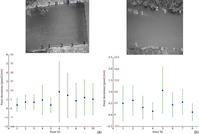
1434 A. Eltner et al.: Flow velocity and discharge measurement in rivers
minimally to find the homography. Again, larger values in-
crease the robustness, but they can also lead to a failure of
processing if fewer feature matches are found than appointed
here. Furthermore, it can be defined which feature descrip-
tor is chosen for matching, if features are matched back and
forth increasing the accuracy and processing time, and if im-
age co-registration is performed to the first frame or in a se-
ries to each consequent frame of the sequence.
2.4.2 Finding features to track
A search area in the river region has to be defined to detect
particles before tracking. This is due to the circumstance that
most feature detectors look for regions with high contrast.
Therefore, points of interest would be found on the land,
where contrast is usually higher than on the water surface.
Thus, in a first step the river area has to be masked in the
images and defined as the search area for tracking before ap-
plying particle detection.
Feature search area and pose estimation
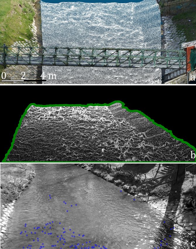
Figure 2. Workflow to retrieve flow velocities from video se- The feature search area is a region of interest that is defined
quences. as a function of the water level to mask the image. The wa-
ter level and a 3D surface model of the river reach (Fig. 3a)
observed by the camera have to be known to define this wa-
all frames to capture the same scene. This processing step ter area automatically. The 3D surface model is clipped with
is preformed fully automatically. In each frame Harris cor- the water level value to solely keep the points below the wa-
ner features are detected (Harris and Stephens, 1988), which ter surface. Afterwards, these points are projected into im-
are then matched to the first frame of the sequence using age space (Fig. 3b). Therefore, information about the pose
SIFT (Lowe, 2004) or ORB descriptors (Rublee et al., 2011). and the interior geometry of the camera is necessary. In the
The suitability of co-registration in different conditions and FlowVelo tool, information about the camera pose is either
over longer periods of time has been illustrated in Eltner et estimated with spatial resection considering the GCP coordi-
al. (2018), who introduce a terrestrial camera gauge for water nates in image and object space and the interior camera pa-
level measurements. rameters (for more details see Eltner et al., 2018) or it can be
Harris features in the water region are detected as out- simply stated if the pose has been defined by other measures.
liers due to their changing appearance between subsequent Next, the 3D point cloud of the observed river reach is
frames leading to matching failure. And if moving features in projected into a 2D image (Fig. 3b). To fill gaps, potentially
the water area still might be matched, they are latest filtered arising for 3D surface models with a low resolution, a mor-
during the parameter estimation of the homography because phological closing is performed. Finally, the contour of the
these points will be considered as outliers during the model underwater area is extracted to define the search mask for the
fitting with RANSAC (random sample consensus; Fischler individual frames. If several contours are detected, the largest
and Bolles, 1981). Thus, only stable and reliable homologous contour is chosen. If a 3D surface model is not present for au-
image points outside the river are kept and used to calculate tomatic feature search area detection, the area of interest for
the homography parameters between the first frame and all tracking can also be provided via a mask file.
subsequent frames. Finally, a perspective transformation is
applied to ensure that all frames fit to the first image. It has Feature detection and filtering
to be mentioned that this approach is only working as long as
enough stable areas are visible on both river shores. Particles are detected with the Shi–Tomasi feature (good
In the FlowVelo tool five parameters can be set to adjust feature to track; GFTT) detector (Shi and Tomasi, 1994).
the co-registration of each individual scenery. The maximum Thereby, features are detected similar to the Harris corner
number of key points defines how many features are max- detector, but a different score is considered to decide for a
imally searched for in each frame. Larger numbers can in- valid feature (Fig. 3c). Many more feature detectors are pos-
crease the robustness and accuracy of matching but also the sible. Tauro et al. (2018) test several methods and show that
processing time. The number of good matches determines the GFTT detector performs well and also finds features in
how many matched features between two frames are needed regions of poor contrast.
Hydrol. Earth Syst. Sci., 24, 1429–1445, 2020 www.hydrol-earth-syst-sci.net/24/1429/2020/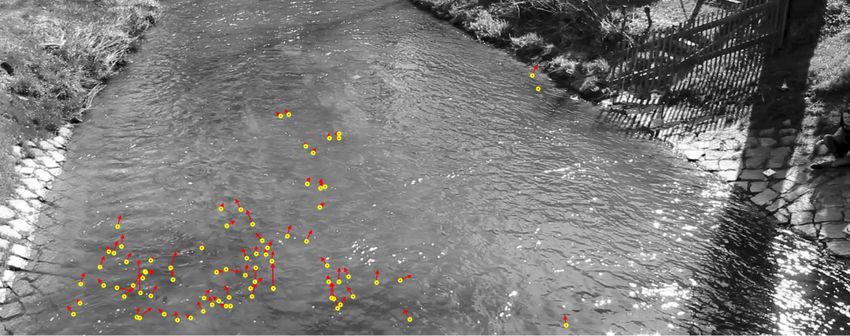
A. Eltner et al.: Flow velocity and discharge measurement in rivers                                                                1435

                                                                       lows accounting for brightness and illumination differences
                                                                       between different frames. The positions of the detected fea-
                                                                       tures are chosen to define templates with a specific kernel
                                                                       size (mostly 10 pixels in this study; Supplement 1). In the
                                                                       next frame NCC is performed within a defined search area
                                                                       (mostly 15 pixels in this study; Supplement 1) to find the
                                                                       positions with highest correlation scores for each feature, po-
                                                                       tentially corresponding to the new positions on the water sur-
                                                                       face of the migrated particles.
                                                                          To refine the matching, an additional sub-pixel accurate
                                                                       processing is performed. Thereby, template and matched
                                                                       search area of the same size are converted into the frequency
                                                                       domain to measure the phase shift between both, and af-
                                                                       terwards the sub-pixel peak location is determined with a
                                                                       weighted centroid fit. The final matched locations define the
                                                                       new templates for tracking in the next frame. This tracking
                                                                       approach is performed for a specified number of frames. In
                                                                       this study, features are tracked for 20 frames, and new fea-
                                                                       tures are detected every 15th frame. It can be suitable to de-
                                                                       tect features more frequently than the number of frames they
                                                                       are tracked across because features can change their appear-
                                                                       ance, and new features can enter the area of view, although
                                                                       the already detected features are still tracked.

                                                                       2.4.4   Track filtering

                                                                       Figure 4 shows that false tracking results can still occur,
Figure 3. Defining the search area to extract particles to track.
                                                                       e.g. tracks that significantly deviate from the main flow di-
(a) 3D point cloud of the investigated river reach at the Wesenitz.
Coloured points (colourised with RGB information according to
                                                                       rection. This is amongst other reasons due to remaining
their real-world object colour) are 3D points above the water sur-     speckle detected as features or due to tracking of features
face reconstructed with SfM photogrammetry. White points are 3D        with a low contrast leading to ambiguous matching scores.
points below the water surface reconstructed with SfM and cor-         Therefore, resulting velocity tracks need to be filtered. Tauro
rected for refraction effects. (b) 3D point cloud below the water      et al. (2018) remove false trajectories considering mini-
level projected into image space. Green line depicts contour line,     mum track length and track orientation. In this study, we
which is used as search mask for feature detection. (c) Detected and   also make assumptions about the flow characteristics of the
filtered features considered for tracking (blue circles).              river (Fig. 5). We consider six parameters: minimum frame
                                                                       amount of a tracked feature, minimum and maximum track-
                                                                       ing distances, flow steadiness, range of track directions, and
   The elimination of particles, which are not suitable for            deviation from the average flow direction. Each track has to
tracking, is necessary. For instance, reflections of sunlight at       fulfil these criteria to be considered as reliable velocity infor-
waves showing high contrasts on the water surface need to              mation. Thereby, each track is the combination of the indi-
be removed to avoid the erroneous tracking of fake particles           vidual sub-tracks from frame to frame, with feature detection
(Lewis and Rhoads, 2015). Therefore, a nearest neighbour               performed in the first frame.
search is performed to find areas with strong clusters of par-            The first criterion considers the minimum percentage of
ticles. If there are too many features within a defined search         frames across which the features have to be traceable (here
radius, the particle will be excluded from further analysis. In        65 %). The underlying assumption is that if the feature is only
addition, features are removed that reveal brightness values           traceable across a few frames, then it is more likely not a
below a threshold, e.g. to avoid the inclusion of wave shad-           well-defined flowing particle at the water surface but may for
ows as features.                                                       instance be a speckle occurrence due to sun glare. However,
                                                                       the minimum value can be set to 0 to avoid any constraints
2.4.3   Feature tracking                                               regarding flow velocities and camera frame rates.
                                                                          The second and third filter criteria are the distances across
When features have been detected, they are tracked through             which features were tracked, comprising thresholds for min-
subsequent frames (Fig. 4). This tracking is performed us-             imum and maximum distances. The distance thresholds can
ing normalised cross-correlation (NCC). Normalisation al-              be roughly approximated when the image scale and the range

www.hydrol-earth-syst-sci.net/24/1429/2020/                                         Hydrol. Earth Syst. Sci., 24, 1429–1445, 2020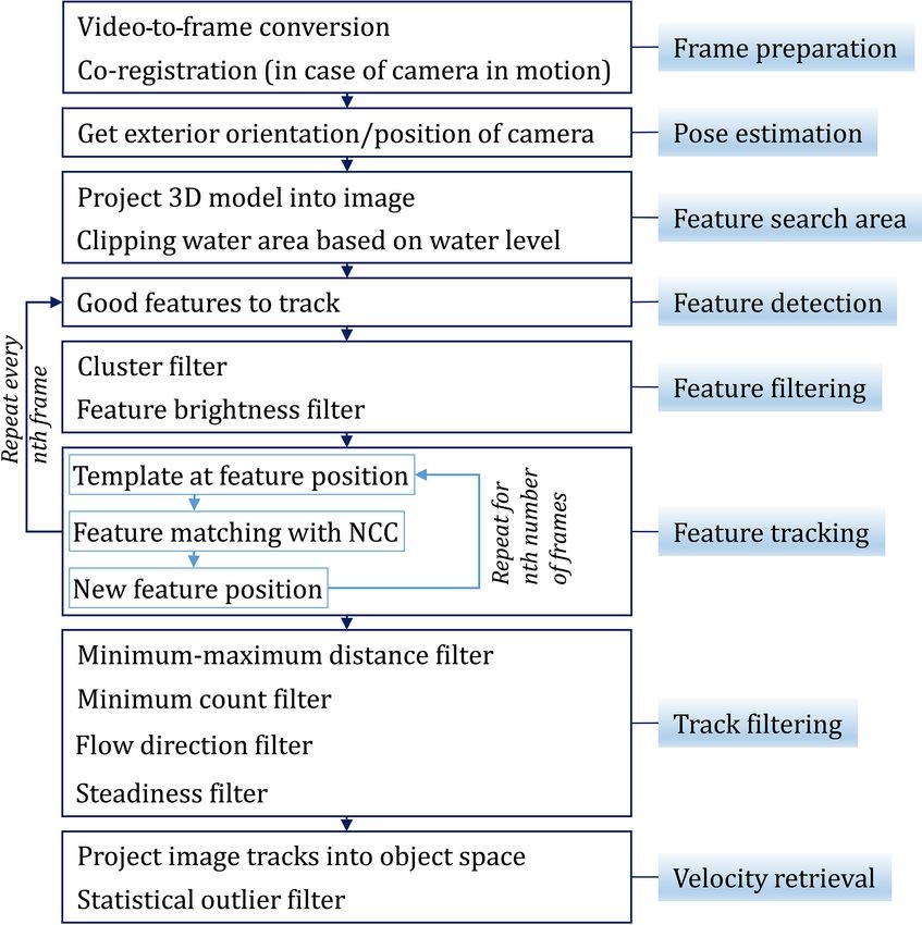
1436                                                        A. Eltner et al.: Flow velocity and discharge measurement in rivers

Figure 4. Exemplary display of the tracking result from one frame to the next.

of expected river flow velocity are known. In this study, the           ending points of each track are intersected with the water
minimum and maximum distance parameters are set to 0.1                  plane to retrieve real-world coordinates. From the distance
and 10 pixels, respectively.                                            between start and end and considering the camera’s frame
   The fourth criterion considers the directional flow be-              rate as well as the number of tracked frames, metric flow ve-
haviour of the feature with a steadiness parameter. Therefore,          locities are retrieved. Finally, the metric velocity tracks are
directions of sub-tracks (from frame to frame) are analysed             filtered once more with a statistical outlier filter to remove
for each track. Tracks are excluded when the standard devi-             remaining outliers (Fig. 6). The threshold is defined as the
ation is above a defined threshold (30◦ in this study). The             sum of the average velocity with a multiple of its standard
idea is that river observations are performed during nearly             deviation (e.g. Thielicke and Stamhuis, 2014). The lower the
uniform flow conditions. Thus, high frequencies of changes              multiple is chosen, the more features will be filtered, and
in flow directions within a track indicate measurement errors           only tracks will be kept which have values close to the aver-
and should be filtered. In addition to this steadiness param-           age velocity. In this study, the parameter was set to 1.5. This
eter, the range of all sub-track directions is also considered          processing step is more important for challenging tracking
as a measure of the flow behaviour. If the range is above a             situations.
defined threshold, the track will be excluded (here 120◦ ).                 Regarding tracking reliability, it should be noted that in
   For the last criterion the main flow direction of the river          the case of terrestrial cameras with an oblique view onto the
is examined. The average direction of all tracks is calculated,         river velocity, measurements are preferred closer to the sen-
and if the direction of the individual tracks are larger or below       sor. Particles move across a larger number of pixels in close
a buffer threshold (here 30◦ ), they are rejected from further          range to the camera than in further distances, e.g. an erro-
processing. The buffer value has to be defined considering              neous measurement of 1 pixel close to the camera might re-
the general variability of the river surface flow pattern. The          sult in a measurement error of 1 cm, whereas at a further dis-
lower the parameter is chosen to be, the more a uniform flow            tance it can correspond to 1 m. Furthermore, tracking accu-
is assumed to be. It has to be noted that the directional filter        racy decreases significantly in far ranges due to increasing
has a limited applicability in more complex flow conditions,            glancing ray intersections with the water surface.
e.g. turbulent, non-uniform rivers. In such situation, local fil-
ters should be preferred over these global values.                      2.5      Discharge estimation

2.4.5   Velocity retrieval                                              The bathymetric information as well as the flow velocities
                                                                        are needed to calculate the discharge. Thereby, sole UAV
In the last processing stage, measured distances are trans-             data can be used as shown by Detert et al. (2017). In this
formed from pixel values to metric units to receive flow ve-            study, we cut river cross sections from the reconstructed
locities in metres per second. With a known camera pose and             bathymetry and topography at the approximate locations of
interior camera geometry, image measurements can be pro-                the ADCP measurements. Afterwards, we extract the water
jected into object space. This leads to a 3D representation of          level information by manually detecting the water line in
the light ray emerging from the image plane and proceed-                at least three overlapping images and spatially intersecting
ing through the camera’s projection centre. 3D object coor-             these point measurements in the object space.
dinates of an image measurement can be calculated by in-                   The surface flow velocity values are averaged and multi-
tersecting its ray with a 3D surface model of the river. In             plied with the velocity coefficients estimated from the ADCP
this case the water surface, assumed to be planar at the water          measurements to account for depth-averaged velocities (Ta-
level, defines the location of intersection. The starting and           ble 1). This approach is suitable at the Wesenitz. But at the

Hydrol. Earth Syst. Sci., 24, 1429–1445, 2020                                          www.hydrol-earth-syst-sci.net/24/1429/2020/
A. Eltner et al.: Flow velocity and discharge measurement in rivers 1437
Figure 5. Result of tracked features after filtering has been applied to the video sequence of the 500D camera (with a temporal length of
23 s). Sub-tracks are displayed, and the number of tracks refers to full tracks (combination of sub-tracks). (a) Raw tracks prior any filtering.
(b) Filtered tracks after applying minimum and maximum distance thresholds. (c) Filtered tracks after applying a minimum count of sub-
tracks over which features need to be tracked. (d) Filtered tracks after considering standard deviation of sub-track directions. (e) Filtered
tracks after considering deviation from average flow direction and the range of orientation angles of sub-tracks. (f) Filtered tracks converted
into metric values to receive flow velocities in metres per second.
Freiberger Mulde the method is restricted due to the irregu- 3.1 Accuracy assessment of camera pose estimation
lar river cross sections limiting the application of a constant and image co-registration
velocity coefficient. Finally, discharge is estimated by multi-
plying the cross-section area with the depth-averaged veloc- To enable an accurate measurement of flow velocities, it is
ity. necessary to consider how well the camera pose has been
estimated. Furthermore, for cameras in motion the accuracy
of frame co-registration has to be evaluated as well, to ensure
3 Results and discussion
that tracked movements of the particles indeed correspond to
In this section, results of the accuracies of the image process- river flow instead of camera movements.
ing are displayed; tracked flow velocities are evaluated; and The accuracy of camera pose estimation can be estimated
discharge estimations are analysed. because more than three GCPs are available. In general, the
camera pose will be calculated more accurately if GCPs are
distributed around the area of interest in the object space and
www.hydrol-earth-syst-sci.net/24/1429/2020/ Hydrol. Earth Syst. Sci., 24, 1429–1445, 20201438 A. Eltner et al.: Flow velocity and discharge measurement in rivers
Figure 6. Accuracy of co-registration of video frames to single master frame displayed in image space (black axis) and the corresponding
accuracy in object space (red axis) at the river Wesenitz (a) and Freiberger Mulde (b). Note that the images are only extracts from the original
(bigger) images.
if images capture them in such a way that they cover the responds to a co-registration accuracy of 4.3±5.2 mm. At the
entire image extent because it allows for a stable image-to- Wesenitz, co-registration reveals an accuracy of 1.0±1.6 pix-
object geometry. Furthermore, for the highest accuracy de- els (6.8 ± 11.3 mm). The lower image coverage of the right
mands, GCPs need to be measured with high accuracy in shore at the Wesenitz leads to a lower quality of the frame co-
object space and ideally with sub-pixel accuracy in image registration when compared to the Freiberger Mulde reach
space. At both river reaches, accuracies are better for the ter- because features for frame matching are only kept outside
restrial cameras (Table 2), which is due to a higher GSD as the water area as the appearance of the river surface changes
cameras are significantly closer to the area of interest com- too quickly. Therefore, higher deviations are measured at
pared to the UAV cameras. At the Wesenitz, another rea- the right shore than at the left shore. Considering only the
son for the larger deviations is the circumstance that well- matched targets at the left river side reveals an error range
marked, artificial GCPs were used for the terrestrial images, similar to the Freiberger Mulde.
whereas GCPs were extracted from the 3D surface models to
estimate the UAV camera pose leading to lower point coor- 3.2 Flow velocity measurements at the Wesenitz
dinate accuracies.
Small template regions (10 pixels in size) in stable areas The tracking results and retrieved flow velocities show a di-
have been chosen (Fig. 6) to estimate the accuracy of frame verse picture for the different cameras. For instance, the final
co-registration. At the Freiberger Mulde only GCPs could be number of flow velocity tracks is different for each device
used as templates because the remaining area of interest is (Table 2). The lowest number of tracks is measured for the
covered by vegetation that changes frequently. At the We- UAV camera. However, this camera solely captured a very
senitz cobble stone corners close to the river surface are cho- short video sequence (about 3 s) that could be used for track-
sen because it is important to see how well co-registration ing. Furthermore, the GSDs of the UAV data are much lower
performs close to the water body for which velocities are es- than the GSD of the terrestrial cameras due to a larger sensor-
timated. Each extracted reference location is tracked through to-object distance. The terrestrial cameras reveal a signifi-
the frame sequence via NCC. In case of a perfect align- cantly denser field of flow velocity tracks (Fig. 7). The ter-
ment, the templates should remain at the same image loca- restrial cameras captured videos of a length of about 0.5 min.
tion throughout the sequence. In this study, at the Freiberger Although video lengths of the terrestrial cameras are simi-
Mulde average deviation between tracked frames to the first lar, the number of final velocity tracks varies. The camera
frame amounts 0.5 ± 0.6 pixels for all templates, which cor- closest to the water surface and with the least oblique view
(1200D-II) reveals the highest track number. The 1200D-I
Hydrol. Earth Syst. Sci., 24, 1429–1445, 2020 www.hydrol-earth-syst-sci.net/24/1429/2020/A. Eltner et al.: Flow velocity and discharge measurement in rivers 1439
Table 2. Accuracy of camera pose estimation and density of tracking results. s0 corresponds to the average reprojection error after the
adjusted spatial resection.
Accuracy Tracking density
s0 Number of Number of Number of final
SD (m) (pixel) frames raw tracks tracks
X Y Z
Wesenitz UAV camera 0.172 0.274 0.162 1.1 78 271 58
500D 0.027 0.066 0.039 0.9 690 3552 439
1200D-I 0.042 0.169 0.080 3.2 700 4781 603
1200D-II 0.041 0.127 0.073 1.6 640 14786 1239
Freiberger Mulde UAV camera 0.085 0.078 0.031 0.5 73 844 126
Casio EX-F1 0.018 0.010 0.015 0.3 750 3886 334
camera reveals a lower number of velocity measurements, Average surface flow velocities from the image-based
although frame resolution and focal length are the same, and measurements are higher or similar to the (extrapolated)
video length is even longer. The third camera (500D) depicts ADCP retrieved surface velocity of 0.7 m s−1 , except for
lowest track number, which is mainly due to a lower frame camera 1200D-II, which depicts lower values, also compared
resolution. to the other cameras (Table 4). A potential reason is the dif-
Besides considerations of the camera geometry, track fil- ferent coverage of the cross section with measured velocity
tering is another very important aspect to retrieve reliable ve- values. 1200D-II reveals the highest velocity value density
locity measurements. The filtered track number is about a and covers a larger part of the cross section (Fig. 7). More
magnitude lower than the raw track amount for the terres- regions with lower velocities are measured by the 1200D-II,
trial cameras (Table 2), highlighting the importance of video whereas the other cameras feature less cross-section cover-
sequences with sufficient temporal duration. Thus, tracking age, and more values are measured in areas of faster veloci-
should be performed as long as possible to increase the ro- ties.
bustness of velocity filtering. Interestingly, an impact of the missing camera calibration
Comparing the range of flow velocity values between the of the UAV images is not obvious. Lens distortion parame-
different terrestrial cameras and the UAV camera reveals a ters were only modelled for the terrestrial cameras but were
good fit (Fig. 7), which also coincides with the ADCP ref- discarded for the UAV camera. The impact is assumed to be
erence (Table 3). Furthermore, regions of faster and slower minimal because the camera distortion is usually especially
velocities are revealed in the terrestrial image data that also large for cameras with very wide angles, which is not the case
show within the acoustic data. The average deviation of all for the UAV camera. Furthermore, the distortion impact is
cameras to the ADCP measurements are calculated for video- more important when features are tracked for large distances
based track values that are within a maximal perpendicular in the image, which is also not the case in this study because
distance to the ADCP profile of 1 m. The difference amounts features are mostly tracked between subsequent frames for
to 0.03±0.06 m s−1 . However, it is difficult to perform an ex- only a few pixels.
act comparison to the ADCP measurements because the pre-
cise location of the ADCP cross section in the local coordi- 3.3 Flow velocity measurements at the Freiberger
nate system of the river reach is not known, as the ADCP boat Mulde
was not equipped with any positioning tool, and its move-
ment across the water surface was neither tracked nor syn- At the Freiberger Mulde a more diverse spatial velocity pat-
chronised. Therefore, accuracy assessment of the spatial ve- tern becomes obvious (Fig. 8). Especially the UAV data re-
locity pattern is limited. Nevertheless, we were able to iden- veal areas of increased and decreased velocities along the
tify the start and end points of the cross sections at the shore river reach. Velocity ranges coincide with the ADCP mea-
in the imagery. Therefore, we could approximately estimate surements. Average deviations of the closest tracks to the
the locations of the cross sections in the decimetre range, reference values (similar to the approach in Sect. 3.2) are
which allows for velocity comparison if the surface flow ve- on average −0.01 ± 0.07 m s−1 for the terrestrial and UAV
locity pattern does not become too variable within the short- camera and for all cross sections. However, velocities are ei-
est distances. This has to be kept in mind when assessing the ther overestimated or underestimated at different profiles and
velocity differences, especially at the Freiberger Mulde. for different cameras (Table 3). The flow velocities for the
UAV data are lower at profile 3 compared to the reference.
However, due to the strong changes of flow velocities within
www.hydrol-earth-syst-sci.net/24/1429/2020/ Hydrol. Earth Syst. Sci., 24, 1429–1445, 20201440 A. Eltner et al.: Flow velocity and discharge measurement in rivers
Figure 7. Flow velocities estimated at the Wesenitz using video frames captured with three different terrestrial cameras and a camera on
a UAV platform. Final tracks after the statistical outlier filter (Fig. 5f) are displayed. Green border indicates area, in which image-based
measurements are compared to ADCP velocities.
Table 3. Deviation between ADCP measurements and video-based flow velocities. Differences are calculated for tracks within a range of
1 m and are closest to the ADCP measurements.
Surface velocity
difference (m s−1 )
Average SD Track count
Wesenitz UAV camera 0.03 0.07 10
500D 0.00 0.06 24
1200D-I 0.02 0.07 56
1200D-II 0.08 0.06 88
Average 0.03 0.06 –
Freiberger Mulde UAV camera Profile 1 0.03 0.09 8
UAV camera Profile 2 0.01 0.06 8
UAV camera Profile 3 −0.05 0.06 8
Casio EX-F1 Profile 1 −0.01 0.05 10
Average 0.01 0.07 –
short distances, especially at cross section 3 (Fig. 1), a pos- values (0.79 versus 0.76 m s−1 , respectively), confirming the
sible reason can be false mapping of ADCP values to image- observations at cross sections 1 and 2.
based values. The assumption that velocity underestimation The terrestrial camera depicts a lower spatial density of ve-
at that cross section is due to imprecise point-based veloc- locities compared to the terrestrial cameras at the Wesenitz
ity comparison is backed when comparing the average cross (Table 2), although the video sequence has a comparable
section UAV-retrieved surface velocity (Table 4) with the av- length. This is due to the significantly lower image resolu-
erage ADCP velocity. In that case, the UAV data reveal larger tion as well as the larger distance to the object. Therefore,
fewer features are detectable. The average flow velocity at
Hydrol. Earth Syst. Sci., 24, 1429–1445, 2020 www.hydrol-earth-syst-sci.net/24/1429/2020/A. Eltner et al.: Flow velocity and discharge measurement in rivers 1441
Table 4. Discharge estimated using flow velocities and cross sections retrieved from UAV data.
Average surface flow velocity at Cross-section Discharge (m3 s−1 )
the cross section (m s−1 ) area (m2 ) Average SD
Wesenitz UAV camera 0.71 4.57 2.73 0.27
500D 0.72 2.76 0.15
1200D-I 0.71 2.72 0.16
1200D-II 0.67 2.58 0.16
Average 2.70 0.18
SD 0.08
Freiberger Mulde UAV camera Profile 1 0.79 11.61 7.34 0.74
Profile 2 0.77 10.35 6.60 0.60
Profile 3 0.79 9.19 5.64 0.43
Casio EX-F1 Profile 1 0.76 11.61 7.06 0.46
Average 6.66 0.56
SD 0.75
Figure 8. Flow velocities estimated at the Freiberger Mulde using video frames captured with a terrestrial camera and a camera on a UAV
platform. Green border indicates area, in which image-based measurements are compared to ADCP velocities.
cross section 1 and the average of contrasted individual ve- 3.4 Camera-based discharge retrieval
locity tracks are smaller than the reference. However, error
behaviour of the image-based data might be less favourable
Discharge estimations at the Wesenitz do not show large
at cross section 1, where the comparison is made for im-
deviations between the cameras because velocity estimates
age tracks measured at the far reach of the image. The sharp
showed low deviations, as well (Table 4). Solely the 1200D-
glancing angles at the water surface lead to higher uncertain-
II camera displays a lower discharge. The average discharge
ties of the corresponding 3D coordinate.
for all cameras amounts to 2.7 m3 s−1 , which corresponds to
The decision about how to set the parameters for tracking
the discharge measured by the ADCP. Deviations to the ref-
(e.g. patch size) and filtering (e.g. statistical threshold) re-
erence are below 4 %, highlighting the great potential of the
mains challenging, especially in long-term applications when
UAV application to retrieve discharge estimates solely from
spatiotemporal flow conditions can change strongly (Hauet
image data in regular river cross sections. Standard devia-
et al., 2008). Thus, in future studies intelligent decision ap-
tions of the discharge estimations due to the consideration
proaches for corresponding parameters need to be developed,
of the standard deviation of the surface flow velocities are
for instance where measurements are performed iteratively
small, ranging from 0.18 m3 s−1 (7 %) to 0.56 m3 s−1 (8 %)
with changing parameters.
at the Wesenitz and Freiberger Mulde, respectively (Table 4).
At the Freiberger Mulde, discharge estimates do not fit as
well to the reference measurements. Velocities are only ob-
served in the main flow of the river, where flow velocities
www.hydrol-earth-syst-sci.net/24/1429/2020/ Hydrol. Earth Syst. Sci., 24, 1429–1445, 20201442 A. Eltner et al.: Flow velocity and discharge measurement in rivers
are higher. Deviations to the ADCP reference are larger for tions. Furthermore, assumptions about the flow characteris-
the terrestrial camera, whose measurements are only com- tics need to be made for successful filtering, which implies
pared to profile 1, which shows a large range of flow velocity either some experience with image velocimetry in riverine
and depicts very low values outside the main flow (Fig. 1). environments or some trials to find the most suitable filtering
Comparing single velocity values to nearby ADCP measure- parameters. Consideration of a suitable choice of the thresh-
ments, instead of comparing averaged cross-section informa- old of the statistical outlier filter is important, as well. If the
tion, reveals that the accuracies of image-based velocity mea- filter is chosen too strictly, it can lead to the loss of valid ve-
surements are indeed higher (Table 3). Neglecting the slower locity tracks, which is especially probable in rivers with com-
flow velocities in the shallower river region outside the main plex flow patterns and a large range of velocities. Another
flow leads to overestimated discharge values for the irregu- important factor of the image velocimetry tool to consider is
larly shaped cross sections, which is in contrast to the regular the impact of the choices of thresholds on processing time.
cross section at the Wesenitz. In addition, using the average On the one hand, the more often features are detected and
velocity coefficient is adverse, because the irregular profile the more frames they are tracked across, the more reliable
shape indicates a changing coefficient (Kim et al., 2008). and robust tracking results are possible because track filtering
Another important issue that needs to be noted is the cir- will receive a larger sample for processing. However, track-
cumstance that the image-based discharge estimation reveals ing more features across an increased number of frames also
a high variability that is sensitive to the defined wetted cross increases processing time significantly, which is especially
section extracted with the defined water level. For instance, relevant for cameras with high frame rates and image reso-
at the Wesenitz already a 1 cm offset in the water level value lutions. Nevertheless, in this study the maximum processing
causes a discharge difference of 0.08 m3 s−1 (3 %), and an time (for the terrestrial cameras at the Wesenitz that captured
offset of 3 cm causes a difference of 7 % (0.2 m3 s−1 ). Dif- videos with lengths of about 0.5 min) was still below 5 min
ferent studies already highlight that the correct water level is on an average computer.
important for accurate discharge estimation due to the wet- Measuring surface velocities implies sensitivities to exter-
ted cross-section area error but that it is less relevant for nal impacts such as winds, waves or raindrops, potentially
the accuracy of the flow velocities due to erroneous ortho- falsifying an already established ratio between surface and
rectification (Dramais et al., 2011; Le Boursicaud et al., average flow velocity, i.e. velocity coefficient, due to decreas-
2016; Leitão et al., 2018). ing or increasing the surface velocity depending on the wind
and wave direction and velocity. However, windy and rainy
3.5 Limits and perspectives conditions should be avoided using any surface velocity mea-
surement. The accuracy and reliability of the surface veloc-
In this study, a workflow for surface flow velocity and dis- ity measurement can be improved by adding traceable par-
charge measurements in rivers using terrestrial and UAV im- ticles to increase the seeding density as shown by Detert et
agery was tested successfully. In general, three main pro- al. (2017). In this study, only natural particles floating at the
cessing steps are necessary, i.e. retrieving terrain informa- river surfaces at both study areas were used, which did not
tion via SfM photogrammetry, estimating the flow velocity cover the entire observed cross section, leading to data gaps
with PTV and eventually calculating the discharge with the complicating the retrieval of discharge from the sparsely dis-
information from both previous steps. However, some con- tributed velocity values.
straints need to be considered. The FlowVelo tool requires The FlowVelo tool does not provide discharge informa-
at least the video frames, the camera pose (either estimated tion, yet, because discharge estimation requires additional
within in the tool considering GCP information or provided parameters which need to be determined prior to using im-
externally), the water level and some estimates of the interior age velocimetry as an accurate automatic remote sensing ap-
camera geometry (at least focal length and sensor size and proach. For instance, the water level and the related cross-
resolution are needed). Furthermore, if the camera was not sectional area are needed, and the velocity coefficient has to
stable during the image acquisition, camera movements can be known, which is a point of uncertainty especially at irregu-
be corrected automatically if sufficient shore areas are visi- lar river reaches. In this study, the velocity coefficient was es-
ble in the frames. With this information and pre-processing, timated from the ADCP measurements dividing the mean ve-
scaled river surface velocities are retrievable fully automati- locity of the cross section with the average surface velocity.
cally. However, alternative approaches, e.g. hydraulic modelling,
However, some characteristics of the tool have to be con- should be analysed in more detail in future studies to evalu-
sidered. One aspect is the shore visibility in the frames for ate if they can support the retrieval of more suitable velocity
the co-registration. To guarantee stable areas that are large coefficients. This becomes especially interesting due to novel
enough at larger rivers, increasing the flying height might possibilities of high-resolution bathymetric and topographic
be necessary, potentially reducing the visibility of features data, e.g. using SfM approaches for river mapping.
to track. Alternatively, cameras with wider opening angles
might be needed, potentially resulting in stronger lens distor-
Hydrol. Earth Syst. Sci., 24, 1429–1445, 2020 www.hydrol-earth-syst-sci.net/24/1429/2020/You can also read