Patterns of nocturnal bird migration in the German North and Baltic Seas - ProBIRD report
←
→
Page content transcription
If your browser does not render page correctly, please read the page content below
Bio
                                                                    Consult
                                                                        SH

ProBIRD report

Patterns of nocturnal bird migration
in the German North and Baltic Seas

Analysis of radar data from offshore wind farms in the German EEZ

Jorg Welcker

Husum, August 2019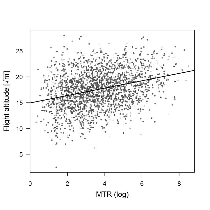
Funded by

                                       Bundesministerium für Umwelt, Naturschutz und nukleare
                                       Sicherheit (BMU)
                                       Stresemannstraße 128-130
                                       10117 Berlin, Germany

Coordinated and supported by

                                       Bundesamt für Seeschifffahrt und Hydrographie (BSH)
                                       Federal Maritime and Hydrographic Agency
                                       Bernhard-Nocht-Straße 78
                                       20359 Hamburg, Germany

The research project “ProBIRD” (FKZ UM15 86 2000) is funded by BMU (Ressortforschungsplan
2015).

Responsibility for the content of this report lies entirely with the authors.

Author

                                       Dr. Jorg Welcker
                                       BioConsult SH GmbH & Co. KG
                                       Schobüller Str. 36
                                       25813 Husum, Germany

Citation

Welcker, J. 2019. Patterns of nocturnal bird migration in the German North and Baltic Seas. Tech-
nical report. BioConsult SH, Husum. 61 pp.

© Bundesamt für Seeschifffahrt und Hydrographie
Image (Title): Kai Gauger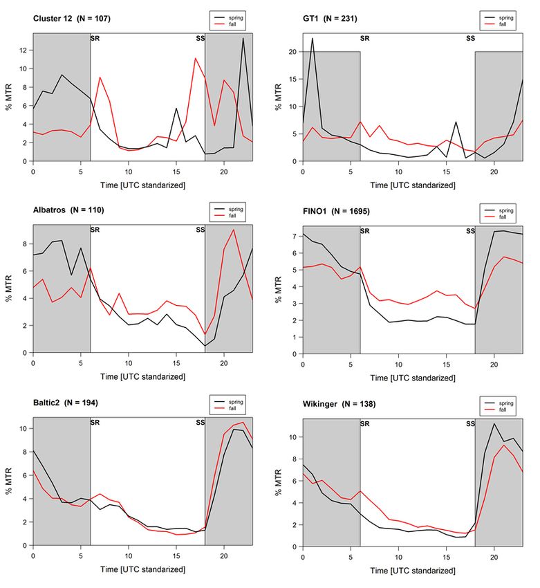
Patterns of nocturnal bird migration in the North and Baltic Sea – ProBIRD report 2

Contents

1          SUMMARY.......................................................................................................................... 1

2          INTRODUCTION .................................................................................................................. 3

3          MATERIALS & METHODS .................................................................................................... 5

3.1        Data collection ................................................................................................................... 5

3.2        Data analysis ...................................................................................................................... 7

3.2.1      Seasonal pattern ................................................................................................................ 9

3.2.2      Spatial correlation of migration intensities ........................................................................ 9

3.2.3      Mass migration .................................................................................................................. 9

3.2.4      Spatial gradients .............................................................................................................. 10

3.2.5      Flight height ..................................................................................................................... 11

3.2.6      Correlation between migration intensities and call rates ................................................ 11

3.2.7      Diurnal pattern................................................................................................................. 11

3.2.8      Estimation of total number of radar signals ..................................................................... 12

4          RESULTS ........................................................................................................................... 13

4.1        Seasonal pattern of bird migration .................................................................................. 13

4.2        Spatial correlation of migration intensities ...................................................................... 16

4.3        Correlation of mass migration ......................................................................................... 18

4.4        Spatial gradients in the German EEZ ................................................................................ 20

4.4.1      Gradient between North and Baltic Sea........................................................................... 20

4.4.2      Gradient with distance to shore within the North Sea ..................................................... 23

4.5        Patterns of flight height ................................................................................................... 25

4.6        Correlation between migration intensities and call rates ................................................ 30

4.7        Diurnal pattern of bird migration ..................................................................................... 31

4.8        Estimation of total number of radar signals ..................................................................... 33

                                                                        i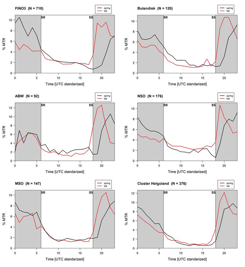
Patterns of nocturnal bird migration in the North and Baltic Sea – ProBIRD report 2

5          DISCUSSION ..................................................................................................................... 35

5.1        Seasonality ....................................................................................................................... 36

5.2        Spatial correlation ............................................................................................................ 37

5.3        Mass migration ................................................................................................................ 37

5.4        Spatial gradient ................................................................................................................ 38

5.5        Flight height ..................................................................................................................... 39

5.6        Correlation between migration intensities and call rates ................................................ 40

5.7        Diurnal pattern ................................................................................................................. 41

5.8        Estimates of the total number of radar signals ................................................................ 41

6          LITERATURE...................................................................................................................... 43

A          APPENDIX ......................................................................................................................... 47

A.1        Spatial correlation of migration intensities ...................................................................... 49

A.2        Correlation of mass migration.......................................................................................... 51

A.3        Gradient of migration intensities ..................................................................................... 52

A.4        Patterns of flight height ................................................................................................... 56

A.5        Estimation of total number of radar signals ..................................................................... 58

A.6        Diurnal patterns of bird migration ................................................................................... 59

List of figures

Figure 3.1 Location of the study sites in the EEZ of the German North and Baltic Sea. .................................5

Figure 3.2 Illustration of the raw radar signals from one year of observations at one radar site. .................7

Figure 3.3 Exemplary illustration of a detection function fitted to two years of data from a radar site. .......8

Figure 3.4 Histogram of mean migration intensities [MTR] (left panel) and log-transformed migration
             intensities (right panel) per night. ...............................................................................................9

                                                                             ii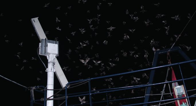
Patterns of nocturnal bird migration in the North and Baltic Sea – ProBIRD report 2
Figure 3.5 Left panel: cumulative MTR [%] per time [%]. Two values are indicated: 45% of radar signals were
recorded in 5% of the nights; 80 % of the radar signals were recorded in 22% of the nights. Right
panel: Mean migration intensities per night sorted in ascending order to illustrate the definition
of ‘mass migration’ (500 MTR) and ‘high migration intensities’ (250 MTR). .............................. 10
Figure 4.1 Seasonal pattern of migration intensities (MTR [migration traffic rate]) in the German EEZ of the
North and Baltic Sea. ................................................................................................................ 14
Figure 4.2 Monthly nocturnal migration intensities [MTR] in the German EEZ of the North and Baltic Sea.
................................................................................................................................................. 15
Figure 4.3 Comparison of the monthly nocturnal migration intensities [MTR] between the North Sea (left
panel) and the Baltic Sea (right panel). ..................................................................................... 15
Figure 4.4 Relationship between distance between sites and the correlation of migration intensities
(Spearman’s rank correlation coefficient rho) for spring (upper panel) and fall (lower panel). .. 17
Figure 4.5 Relationship between distance between sites and the correlation of migration intensities up to
200 m altitude (Spearman’s rank correlation coefficient rho) for spring (upper panel) and fall
(lower panel). ........................................................................................................................... 18
Figure 4.6 Relationship between the distance between sites and the predicted probability [± SE] of
coincidence of high migration intensities at these sites in spring (left panel) and fall (right panel).
Data restricted to North Sea only. ............................................................................................ 19
Figure 4.7 Relationship between the distance between sites and the predicted probability [± SE] of
coincidence of high migration intensities at these sites in spring (left panel) and fall (right panel).
Data from North and Baltic Sea. ............................................................................................... 19
Figure 4.8 Comparison of migration intensities (MTR, log transformed) simultaneously measured in the
Baltic and North Sea. ................................................................................................................ 21
Figure 4.9 Comparison of migration intensities at altitudes up to 200 m (MTR, log transformed)
simultaneously measured in the Baltic and North Sea. ............................................................. 22
Figure 4.10 Comparison of migration intensities (MTR, log transformed) simultaneously measured at two
different sites in the North Sea with different distances to shore. ............................................ 24
Figure 4.11 Relationship of the difference in migration intensities between two sites and their difference in
distance to shore. ..................................................................................................................... 25
Figure 4.12 Distribution of flight heights [%] of nocturnal migrants in the German EEZ of the North and Baltic
Sea in spring (left panel) and fall (right panel)........................................................................... 26
Figure 4.13 Comparison of the distribution of flight heights [%] of nocturnal migrants between the North Sea
(upper panels) and the Baltic Sea (lower panels) in spring (left panels) and fall (right panels). . 26
Figure 4.14 Comparison of the mean flight height per night [m] ±SE between regions (North Sea vs. Baltic
Sea) and between seasons (spring vs. fall) ................................................................................ 27
Figure 4.15 Relationship of the difference in mean flight height [m] between two sites and their difference in
distance to shore. ..................................................................................................................... 28
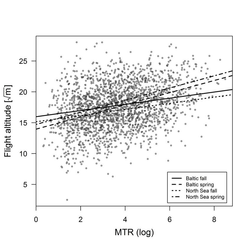
Figure 4.16 Relationship between flight height [m, sqrt-transformed] and migration intensity [MTR, log-
transformed]. ........................................................................................................................... 29
Figure 4.17 Differences in mean flight height [m ±SE] in the course of the night. ........................................ 30
iii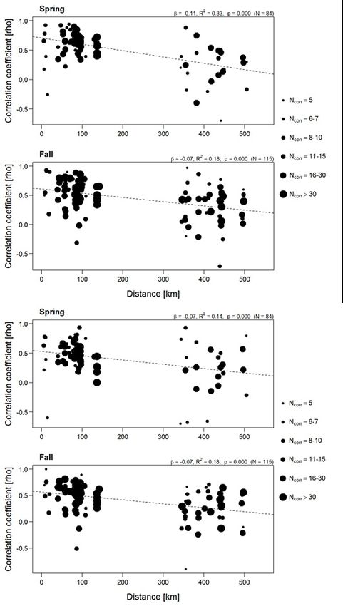
Patterns of nocturnal bird migration in the North and Baltic Sea – ProBIRD report 2

Figure 4.18 Relationship between migration intensity [MTR, log-transformed] and call rates [calls/h, log-
            transformed]. Left panel: MTRs calculated for whole altitude range (0 – 1000m), right panel:
            MTRs up to 200 m altitude. .......................................................................................................31

Figure 4.19 Diurnal pattern of migration intensities [%] in the German EEZ of the North and Baltic Sea. .....32

Figure 4.20 Diurnal pattern of migration intensities [%] in spring (black line) and fall (red line) at different
            areas in the German EEZ. ..........................................................................................................33

Figure A. 1 Relationship between distance between sites and the correlation of migration intensities
            (Spearman’s rank correlation coefficient rho) for spring and fall. Upper two panels: altitude range
            to 1000 m; lower two panels: altitude range to 200 m. .............................................................49

Figure A. 2 Relationship between distance between sites and the correlation of migration intensities
            (Spearman’s rank correlation coefficient rho) for spring and fall). Upper two panels: data
            collected at the same stage of wind farm development (baseline, construction, operation) only;
            lower two panels: by the same lab only. ...................................................................................50

Figure A. 3 Relationship between the distance between sites and the predicted probability [± SE] of
            coincidence of mass migration at these sites in spring (left panel) and fall (right panel)............51

Figure A. 4 Comparison of migration intensities below 200 altitude (MTR, log transformed) simultaneously
            measured at two different sites in the North Sea with different distances to shore. .................52

Figure A. 5 Comparison of migration intensities (MTR, log transformed) simultaneously measured at two
            different sites in the North Sea with different distances to shore as measured perpendicular to
            the assumed migration direction of 45° and 225° in spring and fall, respectively. .....................53

Figure A. 6 Relationship of the difference in migration intensities below 200 m altitude between two sites
            and their difference in distance to shore. ..................................................................................54

Figure A. 7 Relationship of the difference in migration intensities between two sites and their difference in
            distance to shore as measured perpendicular to the assumed migration axis SW-NE (45° and 225°
                in spring and fall, respectively). .................................................................................................54

Figure A. 8 Relationship of the difference in migration intensities between two sites and their difference in
                distance to shore. Data restricted to the same developmental phase of the wind farms...........55

Figure A. 9 Comparison of mean flight height per night [m ±SE] between North Sea and Baltic Sea during the
                months of spring and fall migration. .........................................................................................56

Figure A. 10 Relationship between flight height [m, sqrt-transformed] and migration intensity [MTR, log-
             transformed] for the North and Baltic Sea, and for spring and fall. ...........................................57

Figure A. 11 Diurnal pattern of migration intensities [%] in spring (black line) and fall (red line) in the western
             German Bight.                    59

Figure A. 12 Diurnal pattern of migration intensities [%] in spring (black line) and fall (red line) at different
             OWF locations in the German Bight. .........................................................................................60

Figure A. 13 Diurnal pattern of migration intensities [%] in spring (black line) and fall (red line) at different
             OWF locations in the German EEZ of the North Sea and the Baltic Sea. ....................................61

                                                                                iv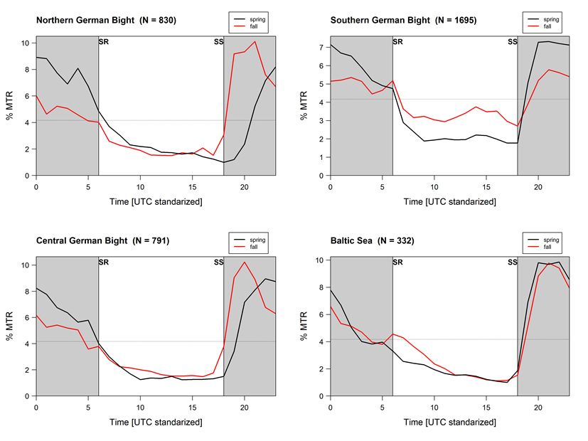
Patterns of nocturnal bird migration in the North and Baltic Sea – ProBIRD report 2

List of tables

Table 3.1   Study sites and sample sizes of the data sets used in this study. ................................................. 6

Table 4.1   Mean migration intensities (MTR, log-transformed ±SE) at the study sites during the different
            developmental stages of the wind farms (baseline, construction and operation). .................... 13

Table 4.2   Mean correlation coefficients (Spearman’s rank correlation coefficient rho) for correlations of
            migration intensities between sites within the North Sea and between sites across the North and
            Baltic Sea. ................................................................................................................................. 16

Table 4.3   Difference in mean nocturnal MTR (log-transformed) between sites in the North and Baltic Sea
            for each month. ........................................................................................................................ 23

Table 4.4   Proportion [%] of radar signals at altitudes below 200 m and below 500 m in spring and fall in the
            German EEZ of the North and Baltic Sea. .................................................................................. 27

Table 4.5   Parameter estimate (slope, β ± SE) and coefficient of determination (R 2) for linear least-squares
            regression of MTRs on bird call rates for each month of the spring and fall migration periods. 31

Table 4.6   Estimated annual total number [±95% CI] of radar signals during spring (01/03 – 31/05) and fall
            (15/07 – 30/11) and during day and night for offshore wind farms in the German EEZ. ............ 34

Tab. A 1    Mean migration intensities (MTR, log-transformed ±SE) at the study sites during the different
            study years. .............................................................................................................................. 47

Tab. A 2    Number of nights per site and year. Only nights for which for at least 75% of the hours radar data
            were available were included in the study ................................................................................ 47

Tab. A 3    Offshore wind farms in the German EEZ for which the total number of radar signals per season
            was estimated. ......................................................................................................................... 58

                                                                           v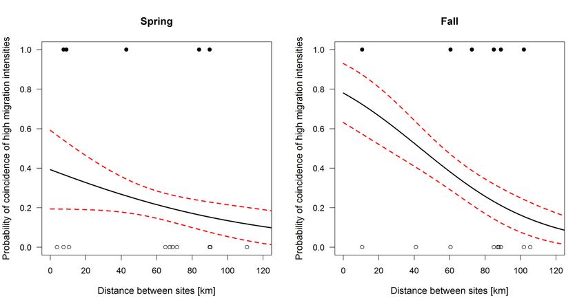
Patterns of nocturnal bird migration in the North and Baltic Sea – ProBIRD report 2

1      SUMMARY
With the advent of offshore wind facilities in the German Exclusive Economic Zone (EEZ) nocturnal
bird migration in these areas has increasingly come into focus. Nocturnally migrating passerines are
often considered to be particularly vulnerable to collisions with offshore wind turbines. Detailed
information on the spatial and temporal patterns of nocturnal migration is of pivotal importance to
assess potential impacts of offshore wind farms (OWFs) on these birds especially since direct data
on bird collisions at offshore turbines are still lacking.

Radar devices are widely used to quantify nocturnal bird movements. This method is also an integral
part of the migration monitoring programs required for environmental impact assessments and
effect studies during construction and operation of German OWFs. Here, we used data from ten
offshore locations in the North Sea and two locations in the Baltic Sea collected over a time period
of nine years (2008 – 2016) to determine spatial and temporal patterns of nocturnal bird migration
in the German EEZ.

Migration intensities (MTRs) showed high day-to-day, inter-annual and between-site variation.
There was little evidence that MTRs varied to any extent between the pre- and post-construction
periods. However, most radar sites were situated up to 3 km outside the wind farm perimeters and
hence might have been too far away to detect potential responses of the birds.

Migration intensities peaked in April and October. The seasonal pattern in fall varied between sites
in the North and Baltic Sea. In the Baltic, MTRs were highest in August and September, but reached
their maximum in the North Sea in October, presumably indicating differences in the main migra-
tory species involved in the two regions.

With a mean correlation coefficient rho of 0.48 the spatial correlation of migration intensities across
all study years and locations was relatively high. Correlation strength decreased only slightly with
increasing distance between sites in the North Sea but was substantially higher within the North
Sea than between the North and Baltic Sea. This suggests that short-term migration patterns were
largely independent between the two regions. Similarly, events of mass migration, defined as mi-
gration intensities >500 MTR, rarely occurred simultaneously at sites in the North and Baltic Sea.

Overall, migration intensities in the Baltic were about 10% higher than in the North Sea, yet this
pattern varied depending on the altitude range and time period considered. Within the North Sea
our results supported the notion of a gradient of migration intensities with distance to shore. MTRs
were significantly lower at sites further offshore compared to sites closer to shore.

Radars recorded bird migration from sea level to 1000 m altitude. Within this range 35% of all flights
were detected below 200 m altitude supporting a number of studies reporting a general prevalence
of low flight heights of nocturnal migrants at sea. Flight heights differed between regions and sea-
sons. In spring, mean flight height in the Baltic was significantly lower than in the North Sea while
the opposite was true in fall. Additionally, at North Sea sites mean flight height was about 100 m
higher in spring compared to fall which might be related to seasonal differences of synoptic wind
conditions. Wind conditions may also account for the fact that flight height at North Sea sites de-
creased with increasing distance to shore, at least in fall.

                                                    1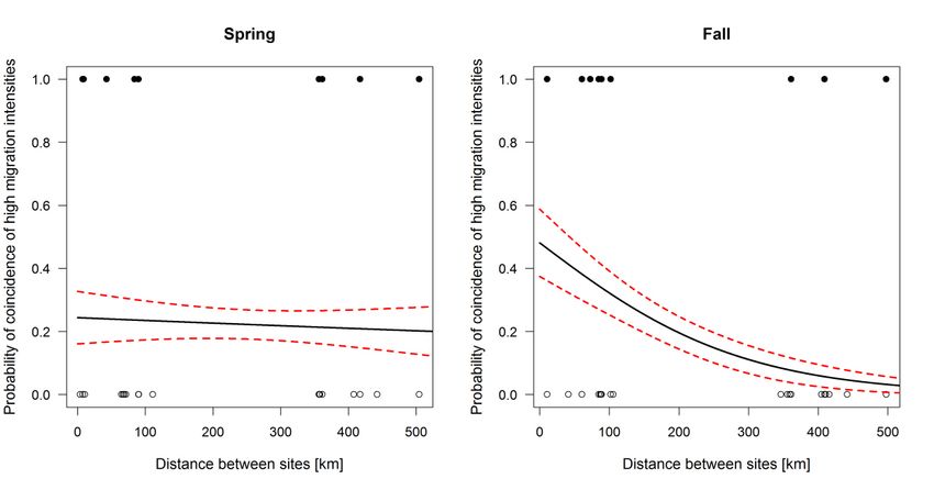
Patterns of nocturnal bird migration in the North and Baltic Sea – ProBIRD report 2

We found that flight heights were positively related to migration intensities. In nights with high
migration intensities flight height tended to be higher than in nights with low migration activity.
This might be the consequence of an increase of both migration activity and flight altitude in re-
sponse to favorable migration conditions. Furthermore, flight heights varied systematically within
the course of the night. At the end of the night, birds flew on average 70 m lower than at its begin-
ning. The reasons for this pattern remain speculative but may be related to an increasing proportion
of birds preparing to land.

Migration intensities observed by radar and the number of flight call of nocturnal migrants, rec-
orded simultaneously at the same sites, were positively correlated. Correlations were strongest in
October and November when most of the migrating species, such as thrushes, are known to be
vocally active.

MTRs showed a strong diurnal pattern. Migration intensities increased sharply shortly after sunset
and peaked before midnight. MTRs decreased again in the second half of the night. Daytime migra-
tion intensity was highest within the first few hours after sunrise. The seasonal variation of this
pattern in different parts of the North Sea was in accordance with the expectation that most noc-
turnal migrants commence migration from coastal areas around sunset.

Finally, we estimated the total number of radar signals (as a proxy for bird movements) passing the
footprints of all 23 German OWFs that are currently operational or under construction each spring
and fall at rotor height at 24 million. Despite several sources of uncertainty, this result suggests that
bird movements at the scale of millions are to be expected at rotor height during the operational
phase of offshore wind farms in the North and Baltic Sea.

                                                     2
Patterns of nocturnal bird migration in the North and Baltic Sea – ProBIRD report 2
2 INTRODUCTION
The majority of migratory birds, particularly passerines, migrate during the night (ALERSTAM 1990,
2009; BERTHOLD et al. 2003). In contrast to diurnal migrants which often concentrate along physical
features of the landscape such as coastlines and which avoid crossing open water, movements of
nocturnally migrating birds are usually spread over wide areas, a pattern called broad-front migra-
tion. On these movements nocturnal migrants regularly fly over large expanses of water like the
North and Baltic Sea.
With the development of offshore wind farms (OWF) in the German Exclusive Economic Zone (EEZ)
of the North and Baltic Sea, nocturnal migration in these areas has increasingly come into focus.
The risk of collision of birds with wind turbines is generally regarded as one of the main potential
impacts of offshore wind developments on wildlife.
Nocturnally migrating birds are often considered as specifically vulnerable to collision with wind
turbines or other anthropogenic structures (LONGCORE et al. 2008, 2012). This risk is thought to be
further increased by inclement weather (rain, fog, poor visibility) and the illumination of the struc-
tures (AVERY et al. 1977; EVANS OGDEN 1996; GEHRING et al. 2009). However, despite the fact that the
first OWFs have been operational for more than 10 years, information on the collision risk of noc-
turnal migrants at OWFs is still scarce. There is strong evidence that nocturnally migrating passer-
ines constitute a large proportion of collision fatalities at illuminated offshore structures such as
platforms where large numbers of birds may collide in single nights (MÜLLER 1981; HÜPPOP et al.
2009, 2016; AUMÜLLER et al. 2011; SCHULZ et al. 2013). On the other hand, there is an increasing
number of studies suggesting that nocturnal migrants incur a rather low risk of collision at onshore
wind facilities (GRÜNKORN et al. 2009, 2016; KRIJGSVELD et al. 2009; WELCKER et al. 2017; but see
ASCHWANDEN et al. 2018). Whether the collision risk of nocturnal migrants at OWFs is similar to that
at onshore wind farms or rather resembles that at other offshore structures remains an open ques-
tion.
This is also due to the fact that nocturnal migration, particularly at sea, is notoriously difficult to
observe. One method increasingly applied is the use of radar. Several different radar systems exist
that are suitable to record bird migration (EASTWOOD 1967; BRUDERER 1997; VAN BELLE et al. 2007;
HÜPPOP et al. 2009; DOKTER et al. 2011; ASSALI et al. 2017; WEISSHAUPT et al. 2018). Most of these
systems allow the quantification of nocturnal migration throughout or for large parts of the height
zone birds are known to migrate in. The accuracy of these data and the comparability between
systems, however, is still debated (WENDELN et al. 2007; SCHMALJOHANN et al. 2008; DOKTER et al.
2013a; MAY et al. 2017; URMY & WARREN 2017; LIECHTI et al. 2018; PHILLIPS et al. 2018; NILSSON et al.
2018). A common property of all radar devices is that they cannot distinguish between species.
For environmental impact assessments as well as subsequent effect monitoring during construction
and operation of OWF in the German EEZ, wind farm developers are required to use marine sur-
veillance radars to collect data on nocturnal bird migration. Radars are operated from vessels or
platforms close to or within the (planned) footprint of the OWFs. Technical specifications of the
devices as well as the main settings are largely standardized by a standard (StUK) issued by the
German Federal Maritime and Hydrographic Agency (Standard – Investigation of the impacts of
offshore wind turbines on the marine environment; BSH 2013). Data collected within this frame-
work were the basis for this study.
3Patterns of nocturnal bird migration in the North and Baltic Sea – ProBIRD report 2
Since the start of OWF developments in Germany several studies have been conducted in order to
increase our understanding of patterns of nocturnal migration in the German EEZ. However, these
studies were often restricted to one or few study sites and usually spanned only a limited time
period (e.g. HÜPPOP et al. 2004, 2006, 2009; OREJAS et al. 2005; BELLEBAUM et al. 2010; SCHULZ et al.
2013, 2014). Therefore, inference about spatial patterns was often difficult and uncertainties re-
mained as to the consistency of observed patterns in time.
In this study we merged the radar data collected within the StUK framework (BSH 2007, 2013) from
12 wind farm sites within the German EEZ from a time period of 9 years. The main aims of the study
were to determine temporal and spatial patterns of nocturnal bird migration in the German North
and Baltic Sea with respect to migration intensities and flight heights and to compare patterns be-
tween the two regions. In addition, results from radar data were compared with those from record-
ings of bird flight calls. Data of flight calls, collected at similar sites and time periods, were analyzed
and reported earlier (WELCKER & VILELA 2018).
This report was prepared within the ProBIRD study (“Prognose des regionalen und lokalen Vo-
gelzugs und des kumulativen Vogelschlagrisikos an Offshore-Windenergieanlagen”) funded by the
Federal Ministry for the Environment, Nature Conservation, and Nuclear Safety (BMU) and sup-
ported by the Federal Maritime and Hydrographic Agency of Germany (BSH).
4Patterns of nocturnal bird migration in the North and Baltic Sea – ProBIRD report 2
3 MATERIALS & METHODS
3.1 Data collection
Radar data were collected at 10 locations in the German EEZ in the south-eastern North Sea (Ger-
man Bight) and at two locations in the Baltic Sea during the years 2008 – 2016 (Figure 3.1). The
different locations were sampled in different years during that period and for different lengths of
time (Table 3.1). Only at one location (FINO1) were data collected during all years of the study pe-
riod. In total the dataset comprised 51 location-years of data (Table 3.1).
Figure 3.1 Location of the study sites in the EEZ of the German North and Baltic Sea.
The data used in this study were collected within bird migration monitoring programs as part of
pre-construction environmental impact assessments as well as effect studies during the construc-
tion and operational phases of offshore wind farms (Table 3.1). Four different companies partici-
pated in data collection. As methods to collect radar data had to comply with requirements issued
by the Federal Maritime and Hydrographic Agency (BSH) as detailed in BSH (2013) data collection
was standardized across the different companies involved.
Within each year data acquisition was restricted to the main migration period in spring and fall
which were defined as the time between 01/03 – 31/05 (spring) and 15/07 – 30/11 (fall). Data were
predominantly collected during ship-based surveys during which the vessels were anchored within
or close (approx. 500 m) to the footprint of the projected wind farm (baseline) or outside the safety
buffer zone (500 - 3000 m) of wind farms under construction or in operation. At locations and dur-
ing time periods where suitable platforms were available these were used as radar sites. This was
the case at FINO1 (2008-2016), FINO3 (2011-2016), Cluster Helgoland (OSS MSO, 2015-2016) and
at Butendiek (2016). FINO1 and FINO3 are located > 1 km outside the nearest wind farm; OSS MSO
is situated centrally within the wind farm while the OSS Butendiek is located at the eastern border
5Patterns of nocturnal bird migration in the North and Baltic Sea – ProBIRD report 2
of the wind farm. Ship-based surveys were carried out for approx. 7 days per month while radars
on platforms ran continuously during the migration periods.
Marine surveillance radars from different manufacturers with the antennas tilted vertically were
used at all study sites. The technical specifications of the radars were in accordance with require-
ments of the StUK (BSH 2007, 2013). The main features of the radars were: power output: 25 kW;
frequency: X-band, 9.41 GHz; horizontal beam width: 0.95° - 1.3°; vertical beam width: 20° - 24° and
pulse length: 0.07 – 0.5 µs. As an exception, a 12 kW X-band radar was used on the FINO1 platform.
The main settings were also standardized by StUK. Rain and sea clutter filters were deactivated as
these functions may also remove bird signals. The reception gain of the radar was set to the highest
possible value which would not lead to interference by static (approx. 70% gain in most cases). The
radar range was set to 1,500 m; the target trail function was set to 25 – 60 s afterglow. Thus, each
radar signal was displayed with a trail of its positions during the afterglow period leading to char-
acteristic bird tracks. At regular intervals (3-5 min depending on project/year) a screenshot of the
radar screen was stored on a hard disk or server. The vertical, horizontal and absolute distance to
the radar of all radar signals considered to represent a bird track was recorded using purpose-built
software. Screenshots with rain clutter masking bird signals were omitted from the analysis.
Table 3.1 Study sites and sample sizes of the data sets used in this study. In addition, seasons (spring or
fall) with available data and the developmental phase of the wind farms during data collection
(B – baseline, C – construction, O – operation) is given.
Radar
Location (output N spring, N fall N nights Years with data Phase (years)
power)
Albatros 25 kW 2,2 124 2008 - 2009 B (2)
Amrumbank West 25 kW 2,2 112 2011 - 2012, 2014 B (2); C (1)
Baltic 2 25 kW 4,5 244 2010, 2013 - 2016 B (1); C (3); O (2)
Butendiek 25 kW 3,3 276 2011, 2014 - 2016 B (1), C (2), O (1)
Cluster Helgoland 25 kW 2,2 424 2015 - 2016 O (2)
FINO1 12 kW 9,9 1772 2008 - 2016 B (1), C (1), O (7)
FINO3 25 kW 4,5 788 2011, 2013 - 2016 B (1), C (2), O (2)
Global Tech I 25 kW 5,6 301 2009, 2012 - 2016 B (1), C (3), O (2)
Cluster 12 25 kW 2,2 118 2009 - 2010 B (2)
Meerwind 25 kW 3,5 181 2010 - 2014 B (2), C (3)
Nordsee Ost 25 kW 3,4 211 2010, 2012 - 2014 B (1), C (3)
Wikinger 25 kW 2,3 154 2014 - 2016 B (2), C (1)
B (16), C (19),
TOTAL 41 , 48 4705 2008 - 2016
O (16)
6Patterns of nocturnal bird migration in the North and Baltic Sea – ProBIRD report 2
3.2 Data analysis
The probability of a bird being detected by radar depends on a variety of factors (BRUDERER 1997).
Most importantly, detectability depends strongly on the distance of the object to the radar. To cor-
rect for distance-dependent detectability, we applied a distance sampling approach as detailed in
HÜPPOP et al.(2006) and WELCKER et al. (2017). This approach is based on the assumption that the
horizontal distribution of migrating birds at sea is uniform. The actual distribution of signals in rela-
tion to the horizontal distance from the radar is therefore thought to reflect the distance-depend-
ent detectability of birds. We selected all radar signals between 50 m and 150 m altitude for the
whole range of 1,500 m (Figure 3.2) and determined the detection function following BUCKLAND et
al. (2001). We fitted models with half-normal and hazard-rate key functions with and without cosine
series expansions up to the fifth order and selected the best model based on Akaike’s information
criterion (AIC). Radar signals were then corrected based on this detection function (Figure 3.3). Dis-
tance correction was done for all radar devices and time periods separately.
Figure 3.2 Illustration of the raw radar signals from one year of observations at one radar site. The grey
semicircle represents the detection range of 1500 m, the white box is the area from which radar
signals were used to calculate MTRs. All signals (black dots) within the altitude range 50 – 150 m
(blue rectangle) were used for modelling the distance-dependent detection probability.
Based on the corrected number of signals, mean migration traffic rates (MTRs – signals*km-1*h-1)
were calculated for each hour of data for which at least three valid screenshots were available. All
signals within 1,000 m horizontal distance from the radar were included (Figure 3.2). MTRs were
calculated for three different altitude ranges: (i) from sea level to 1,000 m a.s.l.; (ii) from sea level
to 200 m a.s.l.; and (iii) for the specific rotor diameters of the wind farms adjacent to each radar
site (see chapter 3.2.7 and Tab. A 3).
7Patterns of nocturnal bird migration in the North and Baltic Sea – ProBIRD report 2
Hourly MTRs were then averaged to derive mean MTRs per night given that hourly values for at
least 75% of the duration of the night were available. Night was defined as the time period between
civil evening twilight and civil morning twilight.
Figure 3.3 Exemplary illustration of a detection function fitted to two years of data from a radar site.
Inspection of the raw radar signals revealed problems in some data sets. The distribution of radar
signals from FINO1 differed noticeably from all other sites. This could be attributed to the fact that
at this site a radar device with different power output (12 kW instead of 25 kW) was used. The
signal distribution led to very high correction factors when correcting for distance-dependent de-
tectability which in turn resulted in considerably higher mean MTRs (see Results, Table 4.1 and Tab.
A 1). Raw data from two other sites, FINO3 and Butendiek during the operational phase, showed
intermittent interferences, presumably with parts of the platforms the devices were installed on,
and with the wind turbines itself (Butendiek), that could not be corrected for. Therefore, data from
FINO1, FINO3 and Butendiek (operational phase) were included in analyses comparing relative
MTRs only (seasonal pattern (chapter 4.1) and spatial correlation (chapter 4.2)) but were omitted
from all other analyses.
8Patterns of nocturnal bird migration in the North and Baltic Sea – ProBIRD report 2
3.2.1 Seasonal pattern
To determine the general seasonal pattern of nocturnal migration in the German EEZ of the North
and Baltic Sea, we calculated mean standardized migration intensities for each Julian day (night).
Migration intensities were log-transformed and standardized across years and sites to avoid uneven
leverage of single years or nights with high flux rates. The seasonal pattern was plotted as a three-
day moving average and as monthly boxplots.
3.2.2 Spatial correlation of migration intensities
To calculate the correlation of migration intensities between sites we first selected all nights with
simultaneous observations in at least two different locations. We then calculated the correlation
coefficient rho based on Spearman’s rank correlation for each pair of sites and years with at least
five nights of simultaneous observations. To determine the spatial variation of the correlation
strength we regressed the correlation coefficients rho against the spatial distance between the lo-
cations for which rho was calculated. The sample size of the pairwise correlations was included as
weights in the regression analysis. This analysis was done for MTRs based on the whole altitude
range and repeated for MTRs up to 200 m height.
3.2.3 Mass migration
We evaluated the possibility to derive a data-driven definition of ‘mass migration’. To this end we
examined histograms and cumulative plots of migration intensities for signs of a bimodal distribu-
tion or any other distribution that would allow the definition of a cut-off value to distinguish be-
tween ‘mass migration events’ and ‘ordinary’ migration intensities.
Figure 3.4 Histogram of mean migration intensities [MTR] (left panel) and log-transformed migration in-
tensities (right panel) per night.
9Patterns of nocturnal bird migration in the North and Baltic Sea – ProBIRD report 2
The distribution of the raw nocturnal flux rates was highly right-skewed, log-transformation re-
sulted in a roughly normal distribution of the data (Figure 3.4). However, both distributions were
continuous and did not show signs of bimodality (Figure 3.3 and Figure 3.4) and hence the definition
of ‘mass migration’ had to be derived independently of the distribution of the data.
We arbitrarily chose the cut-off value for ‘mass migration’ at 500 MTR. ‘High migration intensities’
were defined as > 250 MTR (Figure 3.5). These cut-off values were exceeded in 6.3% and 15.0% of
the nights, respectively. These values were applied to data from all study sites.
We then tested whether the occurrence of mass migration was correlated across locations. To do
so we estimated the effect of distance among sites on the probability of coincidence of mass mi-
gration and high migration intensities as defined above by fitting a generalized linear model with
binomial error distribution and logit link function.
Figure 3.5 Left panel: cumulative MTR [%] per time [%]. Two values are indicated: 45% of radar signals
were recorded in 5% of the nights; 80 % of the radar signals were recorded in 22% of the nights.
Right panel: Mean migration intensities per night sorted in ascending order to illustrate the
definition of ‘mass migration’ (500 MTR) and ‘high migration intensities’ (250 MTR).
3.2.4 Spatial gradients
We tested for a systematic difference in migration intensities between the German EEZ of the North
Sea and the EEZ of the Baltic Sea, and for a gradient with distance to shore within the North Sea. To
determine differences between the North and Baltic Sea we ran paired non-parametric Wilcoxon
tests on migration intensities from nights for which simultaneous observations were available from
both areas. Tests were run for spring and fall separately, for the combined data and for a subset
restricted to simultaneous observations from the same lab. This was done for MTRs of the whole
10Patterns of nocturnal bird migration in the North and Baltic Sea – ProBIRD report 2
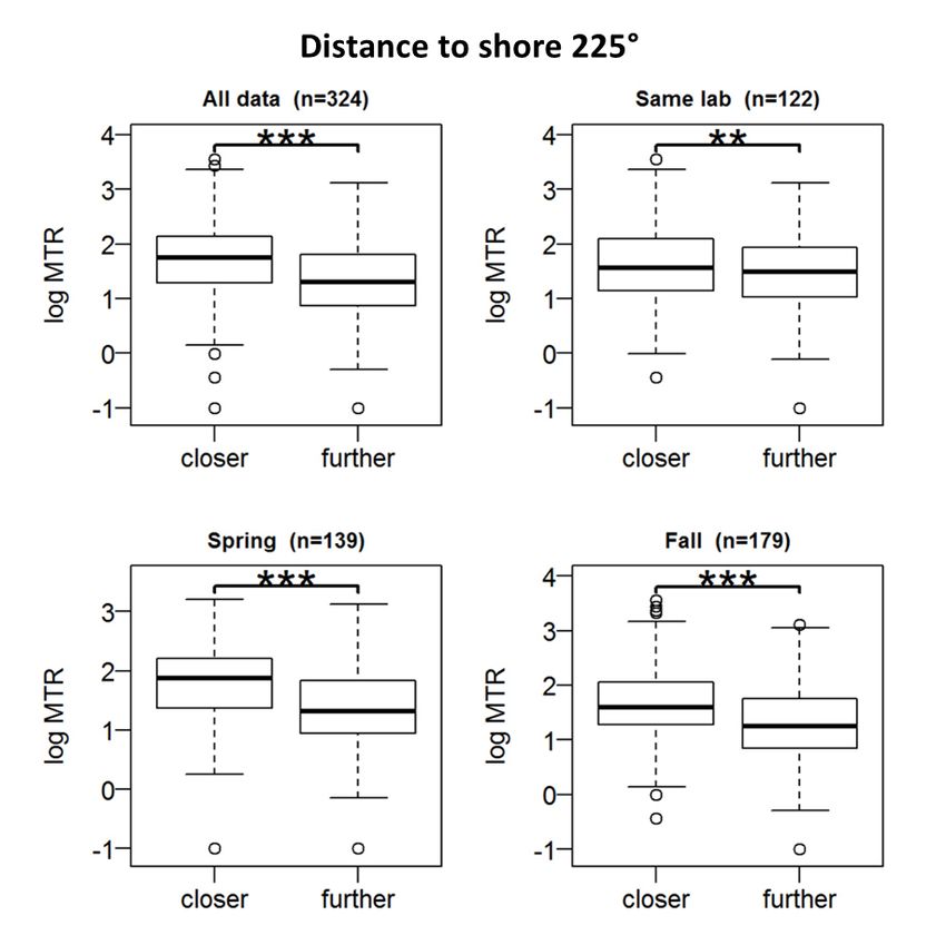
altitude range and for MTRs up to 200 m. Similarly, to determine the gradient with distance to shore
within the North Sea paired Wilcoxon tests were used to compare simultaneously observed MTRs
at sites closer and further away from shore. Additionally, we ran least-squares linear regressions
between the difference in migration intensities between sites and the difference in distance to
shore between these sites. Simultaneous observations with migration intensities of zero at both
sites were excluded prior to the analysis.
3.2.5 Flight height
For the analysis of flight heights, mean flight height per hour of observation in each project was
calculated based on the number of radar signals corrected for distance-dependent detectability.
Mean flight height per night was derived from the mean hourly values. Nights with less than five
raw radar signals were excluded from further analysis.
We tested for differences in mean flight height between seasons (spring vs. fall) and between re-
gions (North Sea vs. Baltic Sea) with an ANOVA including the sum of (corrected) radar signals per
night as weights. To determine whether flight height varied with distance to shore within the North
Sea we ran linear regressions between the difference in flight height between sites and the differ-
ence in distance to shore between those sites. This was done for spring and fall separately. In addi-
tion, a linear regression of flight height on flux rates was fitted with season and region as explana-
tory variables to test for systematic variation of flight heights with migration intensities. Finally, we
examined changes of flight height in the course of the night. To do this, we partitioned each night
in four parts of equal length depending on civil dusk and civil dawn at each location. We then com-
pared the mean flight height in each part of the night using ANOVA.
3.2.6 Correlation between migration intensities and call rates
Data of bird flight calls from the same locations and time periods as the radar data were used to
determine whether call rates of nocturnal migrants and migration intensities estimated by radar
were correlated. Details on the flight call data and the calculation of mean call rates per night can
be found in WELCKER & VILELA (2018).
We ran linear regressions of mean MTR per night on mean flight call rate of simultaneous observa-
tions at the same sites on a log-log scale. Zeros were removed from the dataset. Season was added
as a factor variable to test for differences in correlation strength between spring and fall. Again,
models were run for MTRs calculated for the whole altitude range (up to 1000 m) and for MTRs
below 200 m. A second set of models was fitted for spring and fall separately with month included
as a continuous explanatory variable. In addition, non-parametric Spearman rank correlations were
run on the data including zeros to determine whether the exclusion of zeros in the linear models
was likely to affect conclusions.
3.2.7 Diurnal pattern
To determine the diurnal pattern of bird migration at the offshore sites migration, intensities were
re-calculated based on standardized hours with sunrise set at 06:00 h and sunset at 18:00 h. For
11Patterns of nocturnal bird migration in the North and Baltic Sea – ProBIRD report 2
each site and season mean MTR was then calculated for each standardized hour of the day. Results
were plotted based on relative MTR [%] per hour of the day to allow for a direct comparison of the
diurnal pattern between spring and fall.
3.2.8 Estimation of total number of radar signals
We estimated the total number of birds passing through German OWF each spring and fall based
on the number of radar signals. For each operational wind farm in the EEZ of the North and Baltic
Sea and for each OWF currently under construction the number of radar signals passing through
the footprint of the wind farm at altitudes up to 1000 m, up to 200 m and at the specific rotor height
of each wind farm was calculated as follows:
The total number of signals per night for each night with observations and each site was calculated
by multiplying the mean MTR per night with the length of the night [h] and the maximum extension
of the wind farm [km] perpendicular to the assumed main migration axis (45° and 225° in spring
and fall, respectively) of the birds. All available nightly totals from all study years for a specific wind
farm and season were then taken as the underlying data from which 10,000 bootstrap samples with
replacement were drawn, each sample the length of the respective season (92 days in spring [01/03
– 31/05] and 138 days in fall [15/07 – 30/11]). Then the total sum of signals of each bootstrap
sample was calculated and the mean of the 10,000 sums taken as the estimated number of signals
per season. 95% confidence intervals were derived from the 2.5 th and the 97.5th percentile of the
bootstrap samples. The same procedure was applied to data collected during daytime in order to
derive total estimates for diurnal bird movements.
Not for all focal wind farms data was available. For these wind farms data from the closest radar
site(s) was used for bootstrap sampling instead (Tab. A 3).
12Patterns of nocturnal bird migration in the North and Baltic Sea – ProBIRD report 2
4 RESULTS
Nocturnal migration intensities showed a high day-to-day variability. In addition, mean migration
intensities were highly variable across years and sites (Table 4.1 and Tab. A 1). These two factors
explained 18% of the variance of nocturnal MTRs. Overall, there seemed to be a systematic differ-
ence between the different labs involved in data collection (LM, F2, 1615 = 25.59, p < 0.001). However,
“lab” explained only a small fraction of the variance in MTRs (R 2 = 0.03). Similarly, there was a slight
but statistically significant effect of the developmental stage of the wind farms (LM, F2, 1615 = 3.40,
p = 0.034). During construction, mean MTR was about 8% lower compared to baseline (t = -2.55,
p = 0.011), yet there was no difference between operation and baseline (t = -0.78, p = 0.435). Also,
the explanatory power of the factor “stage” was very low (R2 = 0.004).
Table 4.1 Mean migration intensities (MTR, log-transformed ±SE) at the study sites during the different
developmental stages of the wind farms (baseline, construction and operation).
Baseline Construction Operation
Site
mean log mean log mean log
SE SE SE
MTR MTR MTR
ABW 1.41 ±0.12 1.35 ±0.11
Albatros 1.14 ±0.06
Baltic2 1.34 ±0.16 1.48 ±0.08 1.57 ±0.09
Butendiek 1.29 ±0.10 1.38 ±0.09 0.51 ±0.07
Cluster 12 1.59 ±0.07
Cluster Helgoland 1.53 ±0.05
FINO1 2.37 ±0.04 2.36 ±0.05 2.53 ±0.02
FINO3 0.77 ±0.09 0.49 ±0.04 0.45 ±0.05
GT1 1.67 ±0.11 0.76 ±0.09 1.53 ±0.08
MSO 2.48 ±0.09 1.78 ±0.06
NSO 2.02 ±0.09 1.61 ±0.06
Wikinger 1.73 ±0.08 2.22 ±0.11
Total* 1.58 ±0.03 1.45 ±0.04 1.54 ±0.04
* Totals for wind farm stages were calculated excluding data from FINO1, FINO3 and Butendiek operation. See text for details.
4.1 Seasonal pattern of bird migration
Within both the spring and fall migration periods a clear temporal pattern of nocturnal bird migra-
tion was evident (Figure 4.1 and Figure 4.2). During spring migration intensities increased through-
out March, reached a peak in early/mid-April (maximum value: 09/04) and decreased again during
May (Figure 4.1). Correspondingly, monthly median MTRs were higher in April compared to March
and May (Figure 4.2). This spring pattern was similar in both the North and Baltic Sea (Figure 4.3).
13Patterns of nocturnal bird migration in the North and Baltic Sea – ProBIRD report 2
Figure 4.1 Seasonal pattern of migration intensities (MTR [migration traffic rate]) in the German EEZ of
the North and Baltic Sea. Migration intensities were standardized between years and projects
and plotted as 3-day moving average.
During fall, migration intensities increased slightly from mid-July until mid-September. Highest val-
ues were reached between end of September and early November (maximum: 12/10). In Novem-
ber migration intensities were highly variable yet the number of days with data was considerably
lower than during the other months of the season (Figure 4.1).
The temporal pattern within the fall migration period showed differences between the North and
Baltic Sea. At North Sea sites, migration intensities were generally low at the beginning of the sea-
son in July and August, peaked in October and remained relatively high in November (Figure 4.3).
In contrast, at sites in the Baltic, median MTRs were highest in August and September and de-
creased in October and November.
14Patterns of nocturnal bird migration in the North and Baltic Sea – ProBIRD report 2
Figure 4.2 Monthly nocturnal migration intensities [MTR] in the German EEZ of the North and Baltic Sea.
Box plots indicate the median (bold black bar) and the interquartile range (box), the whiskers
extend to the most extreme data points which are no more than 1.5 times the interquartile
range. Grey circles represent the monthly means.
Figure 4.3 Comparison of the monthly nocturnal migration intensities [MTR] between the North Sea (left
panel) and the Baltic Sea (right panel). See Figure 4.2 for details.
15Patterns of nocturnal bird migration in the North and Baltic Sea – ProBIRD report 2
4.2 Spatial correlation of migration intensities
With a mean correlation coefficient rho of 0.48 ± 0.02 SE (N = 199 correlations) the spatial correla-
tion of migration intensities across all study years and locations was relatively high. However, the
strength of the correlation was significantly higher between sites within the North Sea than be-
tween sites across the North and Baltic Sea (Table 4.2). This was the case for both spring and fall.
Due to the limited dataset from the Baltic, comparisons within the Baltic Sea were not possible.
There was no difference in correlation strength between the seasons (overall: Wilcoxon rank tests,
W = 5282, P = 0.265, North Sea only: W = 1900, p = 0.30).
Generally, the correlation strength of MTRs below 200 m altitude was slightly lower than for the
whole altitude range (0.40 ±0.02 SE vs. 0.48 ±0.02 SE, W = 22330, p = 0.028). Else, the same patterns
with respect to regional and seasonal differences were evident for the data limited to 200 m alti-
tude (Table 4.2)
Table 4.2 Mean correlation coefficients (Spearman’s rank correlation coefficient rho) for correlations of
migration intensities between sites within the North Sea and between sites across the North
and Baltic Sea. In addition, sample sizes (number of correlations within the North Sea and be-
tween the North and Baltic Sea, respectively) and the p-value of Wilcoxon rank tests are given.
Mean rho
Mean rho
Altitude range Season N North Sea Baltic/North N Baltica p
North Sea
Sea
spring 0.61 59 0.21 25Patterns of nocturnal bird migration in the North and Baltic Sea – ProBIRD report 2
Figure 4.4 Relationship between distance between sites and the correlation of migration intensities (Spear-
man’s rank correlation coefficient rho) for spring (upper panel) and fall (lower panel). Correla-
tion coefficients were calculated based on days with simultaneous observations of each pair of
projects and years. The number of days a coefficient is based on is indicated by symbol size
(minimum number of days = 5). Left panel: linear regression for data from the North Sea; right
panel: mean correlation coefficient [± SE] for North Sea sites (open symbol) and for comparisons
between North and Baltic Sea (filled symbols).
17Patterns of nocturnal bird migration in the North and Baltic Sea – ProBIRD report 2
Figure 4.5 Relationship between distance between sites and the correlation of migration intensities up to
200 m altitude (Spearman’s rank correlation coefficient rho) for spring (upper panel) and fall
(lower panel). For details see Figure 4.4 and Materials & Methods.
4.3 Correlation of mass migration
The probability of simultaneous occurrence of high migration intensities decreased significantly
with increasing distance between sites in the North Sea in fall (Figure 4.6, GLM: z = -2.25, p = 0.024)
but not in spring (Figure 4.6, GLM: z = -1.11, p = 0.269). During fall, the predicted probability of
coincidence was about 0.7 – 0.8 for sites in close proximity but declined to about 0.2 at 100 km
distance between sites. Including data from the Baltic led to similar results (Figure 4.7) with a sig-
nificant relationship with distance in fall (GLM: z = -3.19, p = 0.001) but not spring (GLM: z = -0.33,
p = 0.744).
The analysis of simultaneous occurrence of events of mass migration corroborated these results
(Figure A. 3).
18Patterns of nocturnal bird migration in the North and Baltic Sea – ProBIRD report 2
Figure 4.6 Relationship between the distance between sites and the predicted probability [± SE] of coinci-
dence of high migration intensities at these sites in spring (left panel) and fall (right panel). Data
restricted to North Sea only. Predicted probabilities are based on generalized linear models with
binomial error structure (see text for further details). Filled symbols represent distances be-
tween sites at which high migration intensities coincided, open symbols distances at which high
migration intensities did not coincide.
Figure 4.7 Relationship between the distance between sites and the predicted probability [± SE] of coinci-
dence of high migration intensities at these sites in spring (left panel) and fall (right panel). Data
from North and Baltic Sea. Predicted probabilities are based on generalized linear models with
binomial error structure (see text for further details). Filled symbols represent distances be-
tween sites at which high migration intensities coincided, open symbols distances at which high
migration intensities did not coincide.
19Patterns of nocturnal bird migration in the North and Baltic Sea – ProBIRD report 2
4.4 Spatial gradients in the German EEZ
4.4.1 Gradient between North and Baltic Sea
The comparison of simultaneously measured MTRs between sites in the North and Baltic Sea
showed mixed results. Overall, there was a significant difference of migration intensities between
regions with median MTRs in the Baltic being about 10% higher than in the North Sea (Figure 4.8,
paired Wilcoxon rank test: V = 23032, p = 0.013, N = 280). Results for spring (10% difference) and
fall (11% difference) and also for the analysis restricted to data collected by the same lab (14%
difference) were similar, although statistical significance was only reached in fall (Figure 4.8).
Comparisons of MTRs below 200 m altitude showed different results (Figure 4.9). Here there was a
pronounced difference in spring with MTRs in the Baltic being 26% higher than in the North Sea
(V = 4277, p = 0.002). In contrast there was no difference in fall (V = 6714, p = 0.829) indicating dif-
ferences in mean flight heights between seasons and regions (see chapter 4.5).
In addition, the difference in migration intensities between regions varied within seasons (Table
4.3). In spring, migration intensities in the Baltic were higher in April and May while they were
higher in the North Sea in March. There was also a strong monthly pattern in fall with higher MTRs
in the Baltic in August and September but lower MTRs in October and November compared to the
North Sea. There was no difference in July (Table 4.3).
20You can also read