The retrospective analysis of antarctic tracking data project - Nature
←
→
Page content transcription
If your browser does not render page correctly, please read the page content below
www.nature.com/scientificdata

               OPEN           The retrospective analysis of
Data Descri tor               Antarctic tracking data project
                              Yan Ropert-Coudert et al.#

                              The Retrospective Analysis of Antarctic Tracking Data (RAATD) is a Scientific Committee for
                              Antarctic Research project led jointly by the Expert Groups on Birds and Marine Mammals and
                              Antarctic Biodiversity Informatics, and endorsed by the Commission for the Conservation of
                              Antarctic Marine Living Resources. RAATD consolidated tracking data for multiple species
                              of Antarctic meso- and top-predators to identify Areas of Ecological Significance. These
                              datasets and accompanying syntheses provide a greater understanding of fundamental
                              ecosystem processes in the Southern Ocean, support modelling of predator distributions
                              under future climate scenarios and create inputs that can be incorporated into decision
                              making processes by management authorities. In this data paper, we present the compiled
                              tracking data from research groups that have worked in the Antarctic since the 1990s. The
                              data are publicly available through biodiversity.aq and the Ocean Biogeographic Information
                              System. The archive includes tracking data from over 70 contributors across 12 national
                              Antarctic programs, and includes data from 17 predator species, 4060 individual animals, and
                              over 2.9 million observed locations.

                              Background & Summary
                              There is increasing evidence and concern that Southern Ocean ecosystems are facing globally significant chal-
                              lenges, especially in regions undergoing some of the fastest rates of warming on Earth, or where commercial
                              fishing may be impacting ecosystem processes. At lower latitude locations, in the west, such as the Antarctic
                              Peninsula, winter air temperatures have warmed by 4.8 times the global average, and ocean surface tempera-
                              tures have risen by 1 °C1,2. At the same time, concerns about commercial catches of Antarctic krill Euphausia
                              superba and toothfish Dissostichus spp. continue, e.g.3. Ecological effects arising at multiple scales from the phys-
                              ical changes in the environment require further investigations4–6 to allow a realistic assessment of the effects of
                              regional and global warming and ocean acidification vs. top predator recoveries and/or fishing7. The paucity of
                              data on spatial and temporal ecosystem dynamics, and heterogeneity of change even at relatively small spatial
                              scales, e.g.8, adds considerable uncertainty around projections for biological systems. Local mitigation or man-
                              agement measures require a solid knowledge foundation to encapsulate critical ecosystem processes or vulnerable
                              ecosystem components9.
                                  The distributions and abundances of marine endotherms in the Southern Ocean are linked to both habitat
                              and prey availability10. Areas with high concentrations of predators often signal higher diversity or abundance of
                              lower trophic organisms, and are therefore regions that may need special management consideration. In addition
                              to a long history of at-sea surveys, e.g.11, recent advances in electronic tagging techniques provide the capacity to
                              record the movement and behaviour of a range of animals in relation to environmental parameters12. Bio-loggers
                              and transmitters now allow collection of different types of data at the individual level, including geographic loca-
                              tion and environmental data13,14. The use of these devices is now commonplace, leading to an explosion in the
                              quantity and quality of data, creating new challenges for data management, integration, and analysis, and requir-
                              ing the development of new tools and approaches15. Scientists have thus taken advantage of the miniaturisation of
                              electronic tags to remotely follow penguins, petrels, albatross, seals and whales at sea for more than two decades
                              in the Southern Ocean to learn how they spend their time at sea and understand the role they play in different
                              food webs. While lacking a species-interaction context, such data can help to identify regions utilized by multiple
                              species of predators, which are indicative of Areas of Ecological Significance16, or biological hotspots, e.g.17,18.
                                  Despite the considerable number of tracking studies on the distribution and habitat use patterns of upper
                              trophic level, air breathing vertebrates in parts of the Southern Ocean based on tracking data, e.g.19,20, no

                              #
                               A full list of authors and their affiliations appears at the end of the paper.

  Scientific Data |   (2020) 7:94 | https://doi.org/10.1038/s41597-020-0406-x                                                                    1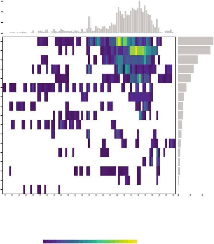
www.nature.com/scientificdata/                                                                      www.nature.com/scientificdata

                               I- Original deployment of tracking devices

                                     Tracking device
                                  deployment on animals                 Tracking           Device specific processing
                                     GLS, PTT, GPS

                                                                                                Step 1

                               II- Data assemblage                     Deployment      Step 2
                                                                        metadata
                                                                                                      Data
                                                                                                    Compilation
                                                                                       Step 3
                                                                       Standardized
                                                       Step 5
                                                                          tracks

                                                                                          Step 4
                                                                                          Filtering and validiation

                                                                                                  Visual Inspection

                                                                                                 duckConfit
                                                                                                 (R package)

                                                                                                      Pre-filter
                                                           DwC-A
                                                          OBIS-ENV
                                                                                                   State specific
                                                                                                    model filter
                                                                              Step 5

                                                                                                Visual quality control
                                                           Filtered
                                                                                                of state space model
                                                           Tracks
                                                                                                    filtered tracks

                            Fig. 1 Data workflow from tracking-device deployment on animals to state-space model-filtered tracks (and
                            associated data). Arrows and boxes correspond to the specific sections in the text. The blue box indicates the
                            filtering and validation workflow for which R scripts are provided; purple boxes indicate publiclyavailable data
                            files through the AADC and Darwin Core packages available through the Global Biodiversity Information
                            Facility (GBIF) and Ocean Biogeographic Information System (OBIS).

                            circum-Antarctic synthesis yet exists that crosses species boundaries. This deficiency prompted the Expert
                            Group on Birds and Marine Mammals (EG-BAMM) and the Expert Group on Antarctic Biodiversity Informatics
                            (EGABI) of the Scientific Committee on Antarctic Research (SCAR; www.scar.org) to initiate in 2010 the
                            Retrospective Analysis of Antarctic Tracking Data (RAATD). RAATD aims to advance our understanding of fun-
                            damental and applied questions in a data-driven way, matching research priorities already identified by the SCAR
                            Horizon Scan9,21 and key questions in animal movement ecology22. For these reasons, we worked on the collation,
                            validation and preparation of tracking data collected south of 45 °S. Data from over seventy contributors (Data
                            Contacts and Citations23) were collated. This database includes information from seventeen predator species,
                            4,060 individuals and over 2.9 million at-sea locations. To exploit this unique dataset, RAATD is undertaking a
                            multi-species assessment of habitat use for higher predators in the Southern Ocean24.
                                RAATD will provide a greater understanding of predator distributions under varying climate regimes, and
                            provide outputs that can inform spatial management and planning decisions by management authorities such as
                            the Commission for the Conservation of Antarctic Marine Living Resources (CCAMLR; www.ccamlr.org). Our
                            synopsis and analysis of multi-predator tracking data will also highlight regional or seasonal data-gaps.

                            Methods
                            Original deployment of tracking devices. RAATD aggregated data from three types of tracking devices
                            (Fig. 1). In increasing order of precision these are light-level recording Global Location Sensors (GLS loggers or
                            geolocators), satellite-relayed Platform Terminal Transmitters (PTTs), and Global Positioning System devices
                            (GPS). Typically, GLS and GPS devices record data in internal memory, and must be physically recovered in order
                            to download the data. PTTs transmit a carrier signal to satellites, and can deliver data remotely and in near-real
                            time. Some modern devices now combine the capabilities of PTT and GPS (or other) devices, relaying high-qual-
                            ity GPS data to the end user via satellites. GLS devices, which are among the smallest, allowing for deployments
                            on smaller predators, typically record ambient light levels throughout the day, from which coarse estimates of
                            latitude and longitude can be calculated (to within 100–200 km) using day length and timing of local noon. Some
                            GLS units can also record sea surface temperature, which can help refine position estimates25. GLS locations were

Scientific Data |   (2020) 7:94 | https://doi.org/10.1038/s41597-020-0406-x                                                                    2
www.nature.com/scientificdata/ www.nature.com/scientificdata
estimated by RAATD data contributors using five methods26–30 (GLS Methods23) and generally corresponded to
individual distribution during the non-breeding season. GPS tags make use of global navigation satellite systems
and provide very high resolution (about ten meters) location fixes and time information. Some are satellite-linked,
while others have smaller batteries and must be recovered (i.e. the animal carrying the tag must be recaptured) to
download the archived data. PTT tags transmit signals to ARGOS satellites which transfer the received signals to
a receiving station at the Collecte de Localisation Satellites (CLS) in Toulouse, France, to estimate locations based
on Doppler shifts in the received signals to an accuracy of approximately 1,000 m. Processing by CLS involved a
least-squares filtering method up to 2008, thereafter Kalman filters have been used31. Different models of GLS,
PTT, and GPS devices from different manufactures have been used throughout the years, each having specific
characteristics (size, operating modes, etc.) that may influence accuracy of the locations, but because device type
was not always provided by the data providers, a standard correction has been applied in RAATD (see below). In
summary, the “RAATD core group” (i.e. the analysing team) worked on location data converted from light-level
data by the data contributors, on CLS-processed PTT location data, and on raw data directly delivered by GPS
devices.
Device attachment to animals was also species-specific. When loggers are small enough, like GLS, they are
mounted on leg or flipper bands/tags, while larger data-loggers and transmitters are often attached to the plumage
or pelage on the back or head of the animal, a position that optimizes data communication with satellites. Modes
of attachment on the back varied from using harnesses, glue or marine tape. For whales, transmitters with subcu-
taneous anchors were attached to the back, using poles, cross bows or air guns. Scientists limited handling time
and stress as much as possible during attachment and retrieval of devices, e.g.32–37, following established animal
handling guidelines that meet ethical reviews. However, it should be noted that the RAATD dataset contains
tracking data that span almost three decades, during which time substantial progress has been made in terms of
miniaturization and advances in electronic components. Any adverse effects of devices on animals are therefore
likely to be less acute in recent years compared to the earlier years of tracking.
Data assemblage. Step 1. data collection. Starting from 2010, RAATD compiled a catalogue of existing
(both published and unpublished) tracking data by contacting international experts that held data. Data were also
harvested from existing repositories, including the Australian Antarctic Data Center (https://data.aad.gov.au/),
the Integrated Marine Observing System (http://imos.org.au/), PANGAEA (https://www.pangaea.de/), BirdLife
International (http://www.seabirdtracking.org/), the Antarctic Biodiversity Portal (http://www.biodiversity.aq/),
Ocean Biogeographic Information System (http://www.iobis.org/), and the Global Biodiversity Information
Facility (http://www.gbif.org/). The data-collection phase ended in 2016.
Step 2. associated metadata. Where available, information on the deployment site and relevant characteristics
of the animal at the time of deployment was standardized. Where age class and sex were known, this information
was included in the metadata.
Step 3. data standardization. Location dates and times were converted to UTC (Coordinated Universal Time).
Records with missing latitude or longitude values were removed, and all longitudes were transformed to lie
between 180 °W and 180 °E. Data files were row-ordered by individual, with rows within an individual in their
correct temporal sequence. Near-duplicate positions, defined as animal positions that occurred three seconds
or less after an existing position fix from the same animal, and which had identical longitude and latitude values
(for GPS devices) or longitude and latitude values that differed by less than 1−05 and which had the same location
quality value (for PTT devices), were removed.
Entries in the age class, breeding stage, device type, location quality, scientific, common, and abbreviated
name, sex, and deployment site columns were validated against controlled vocabularies. Mandatory entries (e.g.,
deployment date, device type, individual animal identifier) were checked for missing values. When the data con-
tributors could not provide missing deployment dates, the first data point of the track was used as a reference
point for deployment. Where animal identifiers were missing, they were created from the the tag identifier or file
name.
Deployment locations were recorded by the original field team either at the individual-animal level (using e.g.,
a hand-held GPS device) or at the deployment-site level (i.e., one deployment location per group of animals). The
latter was common for deployments at colonies, whereas the former was most common for non-colony deploy-
ments (e.g., seals and whales). Where deployment locations were not recorded by the field team, the first location
estimate(s) in the tracking data were used. Deployment site names were standardized to colony names wherever
possible (e.g., to the beach-on-island level).
Periods at the start or end of deployments were identified and discarded if there was evidence that loca-
tion data during these periods did not represent the animals’ at-sea movement. For example, tags may have
been turned on early (thereby recording locations prior to their deployment on animals) or animals may have
remained at the deployment site, e.g. the breeding colony, for an extended period at the start or end of the tag
deployment. Some tracks also showed a marked deterioration in the frequency and quality (for PTTs) of location
estimates near the end of a track. Such locations were visually identified based on maps of each track in con-
junction with plots of location distance from deployment site against time. This information is captured in the
location_to_keep column appended to each species’ raw data file (1 = keep, 0 = discard).
Step 4. data filtering. Each track in the standardized dataset was visually inspected by the Data Editorial Group,
and flagged for removal (using the keepornot column in the metadata file) if location estimates appeared unrea-
sonably noisy relative to the length and extent of the track, and/or the location estimates were very irregular in
time.
Scientific Data | (2020) 7:94 | https://doi.org/10.1038/s41597-020-0406-x 3www.nature.com/scientificdata/ www.nature.com/scientificdata
Next, automated quality-control checks were used to remove individual deployments that: (1) were flagged for
removal (keepornot column in the metadata file); (2) had fewer than twenty location records; or (3) had deploy-
ments lasting less than 1 day. Additionally, individual deployments were checked to ensure that: (1) near-duplicate
records in PTTs (locations occurring within 2 min of each other) were removed; (2) PTT Argos Z-class locations
were reclassified as B-class locations (the least precise Argos location quality class that has an associated error
variance38); and (3) locations implying unrealistic travel rates during the preceding time step (over 10 m s−1 for
penguins and marine mammals and over 30 m s−1 for flying seabirds) were removed. Note that the definition of
“duplicate locations” in the filtering context is more aggressive (less than two minutes vs less than three seconds)
than that used during data standardization: for standardization, the intention was to keep the data as close to
original as possible, whereas for filtering the presence of multiple positions in a short period of time (less than two
minutes) has a negative effect on the filter performance.
A state-space model (SSM) was used to estimate locations at regular time intervals (one hour for GPS data;
two hours for Argos data; twelve hours for GLS data) and account for measurement error in the original observa-
tions12,38. The data were SSM-filtered and subjected to a final quality control where tracks that failed to converge,
as judged by nlminb convergence criteria39, were re-fitted using different initial values. If re-fitted tracks contin-
ued to fail to converge they were removed from the final filtered dataset.
For converged tracks, longitude and latitude residuals were examined for systematic trends indicative of lack
of fit. Tracks that failed this inspection were removed from the final filtered dataset.
Step 5. data publication. RAATD established a data-sharing and publication agreement with all data providers in
2017. The standardized (trimmed) and filtered data are held in a data repository hosted at the Australian Antarctic
Division (AADC) (see details below, in the ‘Standardized Data’ section). The filtered data are also according to the
OBIS-ENV guidelines40 published in international repositories through the SCAR Antarctic Biodiversity Portal
(see details below, in the ‘OBIS-ENV compliant data’ section). For this purpose, and to ensure standardized file
structure, secure (meta)data storage and the facilitation of community access to the data (where appropriate), the
resulting datasets have been uploaded to the biodiversity.aq IPT instance (Integrated Publishing Toolkit; www.
ipt.biodiversity.aq), the accepted route for publishing data to the SCAR Antarctic Biodiversity Portal (www.bio-
diversity.aq). This should ensure a seamless flow to the Ocean Biogeographic Information System (OBIS) and the
Global Biodiversity Information Facility (GBIF).
Data Records
Original data provided by contributors. The original data provided by the data contributors are not
made available here. If needed, the relevant contributors should be contacted; contact details are provided in the
metadata file (columns data_contact and contact_email) and in Data Contacts and Citations23.
Standardized data. Standardized data are provided in files of aggregated comma-separated values (CSV).
They are made available as (i) a single metadata file containing a description for each individual in the dataset and
(ii) a set of seventeen CSV files, one for each species, which aggregate all of the respective individual location data
(Online-only Table 1). Records in the two files can be linked by the common ‘individual_id’ field, as each animal
in the study has a unique identifier. The data and metadata are available to the public through the Australian
Antarctic Data Centre: standardized data41; state-space model-processed (filtered) data42.
OBIS-ENV compliant data. The standardised data will also be provided as a set of Darwin Core Archives
using the Darwincore Event core (Fig. 1) in compliance with the OBIS-ENV-DATA format40. All field definitions
(Darwin Core Terms) are available on the Darwin Core website (at: http://rs.tdwg.org/dwc/terms/index.htm#oc-
currenceindex). The Darwin Core aims to share data about taxa in a simple structured way. It includes a glossary
of terms and is primarily based on their occurrence in nature as documented by observations, specimens, sam-
ples, and related information. Documents describing how these terms are managed, how the set of terms can be
extended for new purposes, and how the terms can be used can be found on the website.
The OBIS-ENV compliant data data are made publicly available through the Antarctic Biodiversity Portal
Integrated Publishing toolkit (http://ipt.biodiversity.aq/resource?r=raatd_scar_trackingdata). The Antarctic
Biodiversity Portal acts as the Antarctic thematic node for the Ocean Biogeographic Information System (OBIS,
Ant-OBIS) and the Global Biodiversity Information Facility (GBIF, AntaBIF).
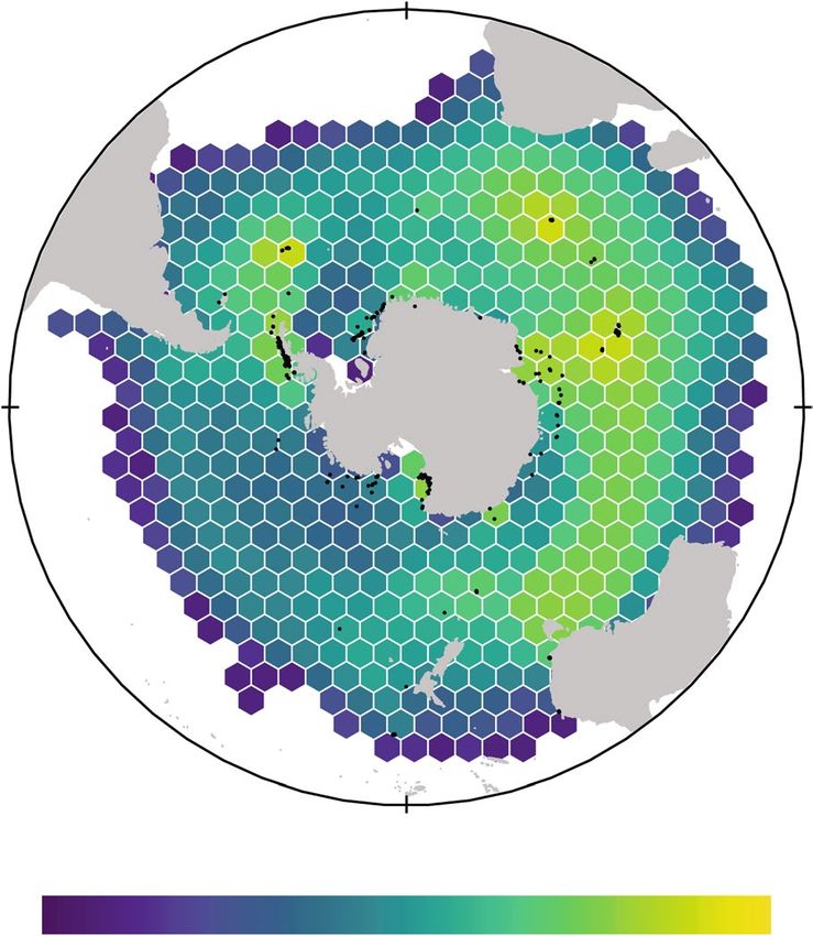
Geographic coverage. All species considered in this dataset have circumpolar Antarctic distributions
(Fig. 2; species-specific distributions are given in Supplementary Fig. S1) with a longitudinal range spanning
180 °W to 180 °E. The species breed either on the coast of the Antarctic continent or on the sub-Antarctic islands
to the north (see Supplementary Table S1 for a list of the main study sites). Species with geographically limited
distributions (such as chinstrap penguins Pygoscelis antarcticus) were not included; instead we concentrated on
species whose distribution covers a large portion of the Southern Ocean. In addition, a number of deployments in
the Antarctic (crabeater seals Lobodon carcinophaga and Weddell seals Leptonychotes weddellii) were conducted
in the pack ice at un-named locations. Similarly, humpback whales Megaptera novaeangliae were instrumented at
sea either off the coast of the Antarctic Peninsula, off Australia or off New Zealand.
Taxonomic coverage. Seventeen species of meso- and top predators were selected for analyses (Table 1 and
Fig. 3), five marine mammals (one baleen whale, one otariid and three phocid seals) and twelve seabirds (five pen-
guins, five albatrosses, and two petrels). These species cover a diverse range of ecological niches and life-history
traits and include dietary specialists (e.g., crabeater seals), deep divers (e.g., elephant seal Mirounga leonina
and emperor penguin Aptenodytes forsteri), wide ranging, highly migratory species (e.g., wandering albatross
Diomedea exulans), nearshore foragers (e.g., Adélie penguin Pygoscelis adeliae) and capital (e.g., Weddell seal)
Scientific Data | (2020) 7:94 | https://doi.org/10.1038/s41597-020-0406-x 4www.nature.com/scientificdata/ www.nature.com/scientificdata
0°
-90° 90°
180°
Number of individuals with location estimates per cell
1 10 100 1000
Fig. 2 Spatial distribution of the number of individuals tracked per 25,000 km2 hexagonal grid cell throughout
the domain of the dataset. Deployment locations are shown with black points. The map is a Lambert Azimuthal
equal area projection, showing the area 90° S to 20° S.
versus income (e.g., Antarctic fur seal Arctocephalus gazella) breeders. In total, 4,060 individuals were included in
the standardized dataset before quality control (some individuals may have been counted more than once in this
total, as repeat deployments on the same individuals are not taken into account in this summation), with 1,482
marine mammals and 2,578 seabirds, providing 2,964,245 location fixes before filtering (Table 1). After filtering
and quality control processes, the total number of individuals used was 2,823, providing 2,328,772 location fixes
(a 21% decrease in the number of location fixes) (Table 1).
Temporal coverage. The data are not distributed evenly in time (Fig. 3). While the time frame ranges from
1991 to 2016, most data were collected during the period 2007 to 2014. This is a reflection of increased research
effort in the Southern Ocean and advances in technology since the early 1990s, and also the timeline of the
RAATD project which stopped actively seeking new data inputs in 2016. Further, some data providers primarily
contributed older datasets that were already published or soon to be published, rather than unpublished data.
The lack of even coverage in terms of taxa, space and time is a function of several factors. First, some deploy-
ments were mostly conducted during the breeding season when species like Adélie penguins make relatively short
duration (2–14 days) and local (10–200 km) foraging trips, compared with post-moulting southern elephant seals
that make distant (several thousands of km) and longer duration foraging trips (many weeks). Second, the cover-
age reflects the research effort related to funding and logistics and, third, the availability of species that lend them-
selves to instrumentation (e.g., central place foragers). For instance, crabeater seals are very abundant but because
they inhabit pack ice they are logistically very difficult to capture for tracking studies. In the case of humpback
whales, long-term attachments of tracking equipment are relatively difficult to attain so there are less data availa-
ble. The technology to track the smaller flying bird species is also comparatively new, relying until recently upon
small archival light loggers (see above), so there have been relatively few studies of these species to date.
Technical Validation
The standardized data were subjected to a range of quality checks before undertaking further processing (Fig. 1).
These included:
• Counts of unique deployment positions and longitude/latitude variability were calculated for each dataset,
and used as a check for errors in deployment position.
• The distance from the recorded deployment position to the first few track points was calculated, and any dis-
tances greater than 10 km were flagged for manual inspection and verification. Similarly, the deployment date
was compared to the date of the first point of the track, and differences were flagged for manual verification.
• Various cross-checks were conducted to identify other data errors or discrepancies, including checking for
multiple device identifiers associated with a single individual animal identifier, checking for identical indi-
vidual identifiers on different species or in different datasets, checking that redeployed devices (i.e. the same
Scientific Data | (2020) 7:94 | https://doi.org/10.1038/s41597-020-0406-x 5www.nature.com/scientificdata/ www.nature.com/scientificdata
Species Standardized data Filtered data
Common name (abbreviation) Scientific name N ind. N fixes N ind. N fixes File name
Total Aves 2,578 1,277,595 1,768 716,057
Aves Adélie penguin (ADPE) Pygoscelis adeliae 820 249,089 520 90,202 RAATD2017_ADPE
Emperor penguin (EMPE) Aptenodytes forsteri 129 74,672 93 104,722 RAATD2017_EMPE
King penguin (KIPE) Aptenodytes patagonicus 117 81,905 109 57,562 RAATD2017_KIPE
Macaroni penguin (MAPE) Eudyptes chrysolophus 505 160,766 182 39,090 RAATD2017_MAPE
Royal penguin* (ROPE) Eudyptes schlegeli 20 4,566 12 3,341 RAATD2017_ROPE
Antarctic petrel (ANPE) Thalassoica antarctica 127 139,603 121 27,957 RAATD2017_ANPE
White-chinned petrel (WHCP) Procellaria aequinoctialis 67 37,606 59 36,875 RAATD2017_WHCP
Wandering albatross (WAAL) Diomedea exulans 276 189,120 253 120,568 RAATD2017_WAAL
Black-browed albatross (BBAL) Thalassarche melanophris 328 144,773 244 161,148 RAATD2017_BBAL
Grey-headed albatross (GHAL) Thalassarche chrysostoma 112 159,547 107 29,501 RAATD2017_GHAL
Sooty albatross (DMSA) Phoebetria fusca 35 14,717 33 23,119 RAATD2017_DMSA
Light-mantled albatross (LMSA) Phoebetria palpebrata 42 21,231 35 21,972 RAATD2017_LMSA
Total Mammalia 1,482 1,686,650 1,055 1,612,715
Mammalia Antarctic fur seal (ANFS) Arctocephalus gazella 555 258,443 313 209,472 RAATD2017_ANFS
Crabeater seal (CRAS) Lobodon carcinophaga 105 83,212 90 89,370 RAATD2017_CRAS
Southern elephant seal (SOES) Mirounga leonina 570 1,013,075 437 913,760 RAATD2017_SOES
Weddell seal (WESE) Leptonychotes weddellii 176 231,967 157 342,563 RAATD2017_WESE
Humpback whale (HUWH) Megaptera novaeangliae 76 99,953 58 57,550 RAATD2017_HUWH
Grand total 4060 2,964,245 2,823 2,328,772
Table 1. Count of the number of individuals and location fixes by species included in the RAATD project
initially (standardized data) and following the cleaning and filtering processes (filtered data). Note, in some
cases (e.g., emperor penguin) the number of fixes of the filtered data is greater than the original number of fixes
in the raw data due to a high prevalence of tag duty-cycling (tags working non-continuously, e.g., recording 12 h
during the day and being turned off for 12 h at night) or due to periods when no location fixes were recorded but
which were interpolated by the state-space model. *Royal penguins have a limited geographic distribution, but
they can be considered ecologically equivalent to Macaroni penguins where they occur, and these two species
will be considered together in RAATD’s further analyses.
device deployed on multiple individuals) did not have temporal overlap, and checking for data missing from
the 29th of February of leap years (perhaps indicating data that had been discarded by accident).
A number of additional quality-control checks were implemented prior to the data filtering; these are
described in the Methods (Steps 3–4). State-space models (SSM) are now the standard approach for dealing
with observation errors in electronic tagging location data38,43. The SSM filtering protocol that was applied to all
the data provided essential quality control and validation. It was a variation of what was used by Jonsen et al.38,
which was implemented in the statistical computing language R44 via the Template Model Builder package (TMB
package)45. The TMB package provides extremely fast and stable maximum likelihood estimation, via autodiffer-
entiation and the Laplace approximation, for non-Gaussian and nonlinear SSM’s46. This was essential for filtering
the large amount of tracking data compiled herein.
The SSM filtering accounted for observation errors in the tracking data and, unlike the raw track data, pro-
vided location estimates and standard errors at regular time intervals along estimated tracks38,47. These location
(error-filtered and time-regularised) outputs are essential for determining species’ habitat preferences from track-
ing data (see Usage Notes) and other types of ecological inferences. We encourage users of these filtered outputs
to evaluate the level of uncertainty in the estimated locations for their ecological inferences, as our methods for
filtering are specific for our purposes. Example filtering code is provided so that users can reproduce our filtered
data from the raw data or produce a new set of filtered data using, for example, different time steps (https://github.
com/SCAR/RAATD).
Following SSM filtering, estimated tracks were evaluated for goodness of fit by examination of (1) maps of esti-
mated and observed locations and (2) residual plots of latitude and longitude. Tracks associated with obviously
poor fits to the data, unrealistic estimated movements and frequent extended periods without observations (rel-
ative to the step length duration) were discarded from the final output dataset. This examination was conducted
independently by three people. Estimated tracks were discarded when at least two examiners were in agreement
to discard. In cases where the optimisation algorithm (nlminb in R) failed to converge to a global minimum, up to
ten attempts with different initial values were made in an effort to obtain convergence. Tracks for which conver-
gence could not be obtained were discarded from the final output dataset. Combined, these quality control and
validation procedures accounted for a 30% reduction in the number of individual tracks retained in the filtered
data compared with the standardized data (Table 1).
The SSM-filtered data are affected by several caveats. First, the standardised GPS, PTT and GLS data were
filtered using time steps of 1-, 2- and 12 h, respectively. These time steps were chosen as they are generally appro-
priate relative to the typical sampling frequencies of the three tag types. In some cases, these time steps did not
Scientific Data | (2020) 7:94 | https://doi.org/10.1038/s41597-020-0406-x 6www.nature.com/scientificdata/ www.nature.com/scientificdata
600
400
200
0
Mirounga leonina
Thalassarche melanophris
Diomedea exulans
Arctocephalus gazella
Leptonychotes weddellii
Pygoscelis adeliae
Procellaria aequinoctialis
Aptenodytes forsteri
Species
Eudyptes chrysolophus
Lobodon carcinophaga
Aptenodytes patagonicus
Megaptera novaeangliae
Thalassarche chrysostoma
Thalassoica antarctica
Phoebetria palpebrata
Phoebetria fusca
Eudyptes schlegeli
0 2000
1992
1993
1994
1995
1996
1997
1998
1999
2000
2001
2002
2003
2004
2005
2006
2007
2008
2009
2010
2011
2012
2013
2014
2015
2016
Year
Number of individual tracking days
50 100 150 200
Fig. 3 Number of individual tracking days (number of individuals with at least one SSM location estimate on a
given day) per species and quarter.
match well with the sampling frequency of particular tags. For example, GPS tags deployed on some birds had far
higher sampling frequencies and a 1-h time step may be too coarse in these cases. Second, for GLS data the time
period around the equinoxes (approximately four weeks, each) yields suspect latitude estimates. The SSM filter
does not fully account for this uncertainty. Third, for animals carrying tags programmed to turn off when hauled
out on land or ice the SSM-estimated locations imply movement looping beyond and back to these haul-out sites
when the tags are off. These estimates are clearly spurious. Fourth, tag-sampling frequency often declines toward
the end of long deployments. Despite some influence on SSM-estimated locations near the end of these deploy-
ments, these data were retained in RAATD.
Usage Notes
Thanks to an unprecedented sharing effort from the SCAR EG-BAMM community, a benchmark dataset has been
assembled that fills important gaps in spatial occurrence of various species for areas of the world that are tradi-
tionally data-poor. The dataset compiled for RAATD is used in the analytical project described in the Background
section to determine Areas of Ecological Significance for the 17 species of predators considered in the dataset.
To this end, a habitat selectivity procedure is one possible modelling method, aiming to identify the particular
environmental conditions that are favoured by the animals, relative to the range of conditions that are available.
This first requires estimation of the geographic space available to a given animal, which can be assessed using
various methods, e.g.48. This region of geographic space has an associated range of environmental conditions over
the period in which animals were tracked. Regression modelling can then be used to identify the environmental
covariates that discriminate areas that are preferentially utilized. For particular analyses, tracking data may need
to be subdivided, for example by breeding stage, depending on whether or not the animals’ interactions with the
environment differ by breeding stage. The individual habitat preference models can then be combined to provide
a multi-species view of important regions of habitat including their underlying environmental processes, e.g.17,18.
Following this analysis and production of a scientific article, the dataset will be available for re-use to help address
emerging research questions or pressing conservation issues.
The SCAR EG-BAMM is pleased to make this dataset openly available for the Antarctic and broader scientific
communities. It is organized and curated using the best principles and practices of recent biodiversity infor-
matics practices49. In this framework, the final version of the dataset is fully compliant with Darwin Core body
of standards and can be downloaded through the Global Biodiversity Information Facility (GBIF) and Ocean
Biogeographic Information System (OBIS) data portals.
In regard to the use of the dataset, the RAATD consortium promotes the CC-BY (Creative Commons
Attribution License), this being the standard practice for citing GBIF-mediated data, believing that it reflects
an established norm that the communities we serve use to cite original work. Users are expected to comply with
the guidelines of the SCAR/SCADM Data Policy: https://www.scar.org/scar-library/reports-and-bulletins/
scar-reports/2717-scar-report-39/file/ and to recognize the valuable contributions of data providers (generally
Scientific Data | (2020) 7:94 | https://doi.org/10.1038/s41597-020-0406-x 7www.nature.com/scientificdata/ www.nature.com/scientificdata
scientists who collect, synthesise, model, or prepare analysed data) and to facilitate repeatability of research
results. Users of SCAR data should communicate with and formally acknowledge data authors (contributors)
and sources, refer to Data Contacts and Citations23, for specific citations. Where possible, this acknowledgment
should take the form of a citation, such as when citing a book or journal article.
Code availability
The code for (i) trimming the raw tracks and (ii) the state space filtering have been made available on the SCAR
github page (https://github.com/SCAR/RAATD). Additional information is provided in the Technical Validation
section below.
Received: 22 May 2018; Accepted: 12 October 2018;
Published: xx xx xxxx
References
1. Gutt, J. et al. The Southern Ocean ecosystem under multiple climate change stresses - an integrated circumpolar assessment. Glob.
Change Biol. 21(4), 1434–1453 (2015).
2. Turner, J. et al. Antarctic Climate Change and the Environment – 2016. (SCAR), http://www.scar.org/scar_media/documents/
policyadvice/treatypapers/ATCM39_ip035_e.pdf (2016).
3. Abrams, P. A. et al. Necessary elements of precautionary management: implications for the Antarctic toothfish. Fish & Fish. 17,
1152–1174 (2016).
4. Barnes, D. K. A. & Peck, L. S. Vulnerability of Antarctic shelf biodiversity to predicted regional warming. Clim. Res. 37, 149–163
(2008).
5. Trathan, P. N. & Agnew, D. Climate change and the Antarctic marine ecosystem: an essay on management implications. Antarct. Sci.
22, 387–398 (2010).
6. Ingels, J. et al. Possible effects of global environmental changes on Antarctic benthos: a synthesis across five major taxa. Ecol. Evol. 2,
453–485 (2012).
7. Trathan, P. N. et al. Pollution, habitat loss, fishing, and climate change as critical threats to penguins. Conserv. Biol. 29(1), 31–41
(2014).
8. Stammerjohn, S., Massom, R., Rind, D. & Martinson, D. Regions of rapid sea ice change: An inter-hemispheric seasonal comparison.
Geophys. Res. Lett. 39(6) (2012).
9. Kennicutt, M. C. et al. Six priorities for Antarctic science. Nature 512(7512), 23–25 (2014).
10. Ropert-Coudert, Y. et al. In Biogeographic Atlas Of The Southern Ocean (eds. De Broyer, C., Koubbi, P., Griffiths, H., Raymond, B.,
d’Udekem d’Acoz, C., Van de Putte, A., Danis, B., David, B., Grant, S., Gutt, J., Held, C., Hosie, G., Huettmann, F., Post, A. & Ropert-
Coudert, Y.) Ch. 8 (SCAR, Cambridge, 2014).
11. De Broyer C. et al. Biogeographic Atlas of the Southern Ocean (Cambridge, Scientific Committee on Antarctic Research, 2014).
12. Block, B. A. et al. Tracking apex marine predator movements in a dynamic ocean. Nature 475(7354), 86–90 (2011).
13. Ropert-Coudert, Y. & Wilson, R. P. Trends and perspectives in animal-attached remote-sensing. Frontiers Ecol. Environ. 3, 437–444
(2005).
14. Treasure, A. M. et al. Marine Mammals Exploring the Oceans Pole to Pole: A review of the MEOP consortium. Oceanography 30(2),
132–138 (2017).
15. Hussey, N. E. et al. Aquatic animal telemetry: A panoramic window into the underwater world. Science 348, 1255642 (2015).
16. Hindell, M. A. et al. In The Kerguelen Plateau: marine ecosystem and fisheries (eds. Duhamel, G. & Welsford, D.) (Paris, Société
Française d’Ichtyologie, 2011).
17. Raymond, B. et al. Important marine habitat off east Antarctica revealed by two decades of multi-species predator tracking.
Ecography 38, 121–129 (2015).
18. Reisinger, R. R. et al. Habitat modelling of tracking data from multiple marine predators identifies important areas in the Southern
Indian Ocean. Divers. Distributions 24, 535–550 (2018).
19. Ballard, G. et al. Responding to climate change: Adélie penguins confront astronomical and ocean boundaries. Ecology 91,
2056–2069 (2010).
20. Delord, K. et al. Areas of importance for seabirds tracked from French southern territories, and recommendations for conservation.
Mar. Policy 48, 1–13 (2014).
21. Xavier, J. C. et al. Future Challenges in Southern Ocean Ecology Research. Frontiers Mar. Sci. 3, 94 (2016).
22. Hays, G. C. et al. Key Questions in Marine Megafauna Movement. Ecology. TREE 31, 463–475 (2016).
23. Ropert-Coudert, Y. et al. The Retrospective Analysis of Antarctic Tracking Data Project. figshare. https://doi.org/10.6084/
m9.figshare.c.4246466 (2018).
24. Hindell, M. A. et al. Tracking predator communities to protect the Southern Ocean. Nature. https://doi.org/10.1038/s41586-020-
2126-y (2020).
25. Merkel, B. et al. probabilistic algorithm to process geolocation data. Mov. Ecol. 4, 26 (2016).
26. Phillips, R. A., Silk, J. R. D., Croxall, J. P., Afanasyev, V. & Briggs, D. R. Accuracy of geolocation estimates for flying seabirds. Mar.
Ecol. Prog. Ser. 266, 265–272 (2004).
27. Sumner, M. D., Wotherspoon, S. J. & Hindell, M. A. Bayesian Estimation of Animal Movement from Archival and Satellite Tags.
PLoS ONE 4(10), e7324 (2009).
28. Lisovski, S. & Hahn, S. GeoLight - processing and analysing light-based geolocator data in R. Methods Ecol. Evol. 3, 1055–1059
(2012).
29. Bindoff, A. geolocationHMM. GitHub, https://github.com/ABindoff/geolocationHMM (2017).
30. Wotherspoon, S. SGAT. GitHub, https://github.com/SWotherspoon/SGAT (2017).
31. Lopez, R., Malarde, J. P., Royer, F. & Gaspar, P. Improving Argos doppler location using multiple-model Kalman filtering. IEEE
Trans. Geosci. Remote Sens. 52(8), 4744–4755 (2014).
32. Bannasch, R., Wilson, R. P. & Culik, B. Hydrodynamic aspects of design and attachment of a back-mounted device in penguins. J.
Exp. Biol. 194(1), 83–96 (1994).
33. Walker, B. G. & Boveng, P. L. Effects of time–depth recorders on maternal foraging and attendance behavior of Antarctic fur seals
(Arctocephalus gazella). Can. J. Zool. 73, 1538–1544 (1995).
34. Phillips, R. A., Xavier, J. C. & Croxall, J. P. Effects of satellite transmitters on albatrosses and petrels. The Auk 120(4), 1082–1090
(2003).
35. McCafferty, D. J., Currie, J. & Sparling, C. E. The effect of instrument attachment on the surface temperature of juvenile grey seals
(Halichoerus grypus) as measured by infrared thermography. Deep Sea Res. Part 2 Top. Stud. Oceanogr. 54(3-4), 424–436 (2007).
36. Vandenabeele, S. P., Shepard, E. L., Grogan, A. & Wilson, R. P. When three per cent may not be three per cent; device-equipped
seabirds experience variable flight constraints. Mar. Biol. 159(1), 1–14 (2012).
37. Field, I. C. et al. Refining instrument attachment on phocid seals. Mar. Mammal Sci. 28, E325–E332 (2012).
Scientific Data | (2020) 7:94 | https://doi.org/10.1038/s41597-020-0406-x 8www.nature.com/scientificdata/ www.nature.com/scientificdata
38. Jonsen, I. D., Flemming, J. M. & Myers, R. A. Robust State-Space modeling of animal movement data. Ecology 86, 2874–2880 (2005).
39. Nash, J. C. On best practice optimization methods in R. J. Stat. Softw. 60(2), 1–14 (2014).
40. De Pooter, D. et al. Toward a new data standard for combined marine biological and environmental datasets - expanding OBIS
beyond species occurrences. Biodiv. Data J. 5, e10989 (2017).
41. Ropert-Coudert, Y. et al. Standardized Data from the Retrospective Analysis of Antarctic Tracking Data Project from the Scientific
Committee on Antarctic Research. Australian Antarctic Data Centre, Australia. https://doi.org/10.4225/15/5afcb927e8162 (2018).
42. Ropert-Coudert, Y. et al. Filtered Data from the Retrospective Analysis of Antarctic Tracking Data Project from the Scientific
Committee on Antarctic Research. Australian Antarctic Data Centre, Australia. https://doi.org/10.4225/15/5afcadad6c130 (2018).
43. Johnson, D. S., London, J. M., Lea, M. A. & Durban, J. W. Continuous-time correlated random walk model for animal telemetry data.
Ecology 89, 1208–1215 (2008).
44. R version 3.3.1, The R Foundation for Statistical Computing (2016).
45. Kristensen, K., Nielsen, A., Berg, C. W., Skaug, H. & Bell, B. M. TMB: automatic differentiation and Laplace approximation. J. Stat.
Softw. 70, 1–21 (2016).
46. Albertsen, C. M., Whoriskey, K., Yurkowski, D., Nielsen, A. & Mills Flemming, J. Fast fitting of non-Gaussian state-space models to
animal movement data via Template Model Builder. Ecology 96, 2598–2604 (2015).
47. Jonsen, I. D. et al. State-space models for bio-loggers: A methodological road map. Deep-Sea Res. II 88-89, 34–46 (2013).
48. Wakefield, E. D. et al. Habitat preference, accessibility, and competition limit the global distribution of breeding Black-browed
Albatrosses. Ecol. Monogr. 81, 141–167 (2011).
49. Parsons, M. A. et al. A conceptual framework for managing very diverse data for complex, interdisciplinary science. J. Inf. Sci. 37(6),
555–569 (2011).
Acknowledgements
The RAATD project would not have been possible without the dedication of the many scientists, students and
field assistants who helped collect data in the field or process them, including, non-exhaustively, S. Adlard,
A. Agüera, M. Biuw, M.-A. Blanchet, J. Clarke, P. Cock, H. Cox, M. Connan, A.R. Carlini, S. Corsolini, M.
Cottin, J.D. Le Croquant, G.A. Danieri, D. Davies, B. Dilley, R. Downie, M. Dunn, B.M. Dyer, H.O. Gillett, S.
Haaland, L. Jonsen, B.A. Krafft, C. Kroeger, C.A.E. Lemon, G. Mabille, M. Marczak, T. McIntyre, J.A. Mennucci,
T. Nordstad, C. Oosthuizen, R. Orben, F. Pezzo, T. Photopoulou, B. Picard, O. Prud’homme, T. Raclot, S.
Ramdohr, D.H. Raymond, G. Robertson, T. Rogers, K. Ropert-Kato, S. Schoombie, E. Soininen, A. Specht, K.
Stevens, J.N. Swærd, C. Tosh, S. G. Trivelpiece, O. S. G. Trolli, L. Upfold, M. Le Vaillant, Y. Watanabe, M. Wege,
C. Wheeler, T.O. Whitehead, M. Widmann, A.G. Wood, N. Youdjou and I. Zimmer. We extend our thanks to
the large number of fieldworkers without whom these valuable data would not have been collected. Support and
funding were provided by supranational committees and organisations including the Scientific Committee on
Antarctic Research Life Science Group and BirdLife International, as well as from various national institutions
(see also author affiliations) and foundations, including but not limited to Argentina (Dirección Nacional del
Antártico), Australia (Australian Antarctic program; Australian Research Council; Sea World Research and
Rescue Foundation Inc., IMOS is a national collaborative research infrastructure, supported by the Australian
Government and operated by a consortium of institutions as an unincorporated joint venture, with the University
of Tasmania as Lead Agent), Belgium (Belgian Science Policy Office, EU Lifewatch ERIC), Brazil (Brazilian
Antarctic Programme; Brazilian National Research Council (CNPq/MCTI) and CAPES), France (Agence
Nationale de la Recherche; Centre National d’Etudes Spatiales; Centre National de la Recherche Scientifique;
the French Foundation for Research on Biodiversity (FRB; www.fondationbiodiversite.fr) in the context of the
CESAB project “RAATD”; Fondation Total; Institut Paul-Emile Victor; Programme Zone Atelier de Recherches
sur l’Environnement Antarctique et Subantarctique; Terres Australes et Antarctiques Françaises), Germany
(Deutsche Forschungsgemeinschaft, Hanse-Wissenschaftskolleg - Institute for Advanced Study), Italy (Italian
National Antarctic Research Program; Ministry for Education University and Research), Japan (Japanese
Antarctic Research Expedition; JSPS Kakenhi grant), Monaco (Fondation Prince Albert II de Monaco), New
Zealand (Ministry for Primary Industries - BRAG; Pew Charitable Trusts), Norway (Norwegian Antarctic
Research Expeditions; Norwegian Research Council), Portugal (Foundation for Science and Technology), South
Africa (Department of Environmental Affairs; National Research Foundation; South African National Antarctic
Programme), UK (Darwin Plus; Ecosystems Programme at the British Antarctic Survey; Natural Environment
Research Council; WWF), and USA (U.S. AMLR Program of NOAA Fisheries; US Office of Polar Programs).
Author contributions
M.A.H. conceived and led the project. H.B., J.-B.C., B.D., M.A.H., L.A.H., I.J., M.A.L., B.R., R.R.R., Y.R.C., D.T.,
L.G.T., P.N.T., A.V.d.P. and S.W. are core members of RAATD. D.G.A., R.A., B.A., G.B., J.B., M.N.B., L.B., H.B.,
C.-A.B., P.B., J.-B.C., R.C., D.P.C., R.J.M.C., L.D.R., P.J.N.d.B., K.D., S.D., M.D., K.D., L.E., M.F., A.F., N.G., M.G.,
K.T.G., C.G., S.D.G., R.H., J.H., M.A.H., L.A.H., A.K., K.R.K., R.K., G.L.K., K.M.K., K.L., A.L., C.L., M.A.L., P.L.,
A.B.M., M.E.I.M., B.M.c.D., C.M.c.M., M.M., K.N., E.S.N., S.O., R.A.P., P.P., J.P., K.P., N.R., Y.R.C., P.G.R., M.S.,
A.S.B., C.S., I.S., A.T.a.k., A.T.a.r., L.G.T., P.N.T., W.T., E.W., H.W., B.W. and J.X. collected and contributed data.
V.A.-G., H.B., J.-B.C., B.D., M.A.H., L.A.H., K.J., A.K., I.J., M.A.L., D.N., B.R., R.R.R., Y.R.C., D.T., L.G.T., P.N.T.,
A.V.d.P. and S.W. processed and analysed the data. H.B., J.-B.C., B.D., M.A.H., L.A.H., I.J., M.A.L., B.R., R.R.R.,
Y.R.C., D.T., L.G.T., P.N.T., A.V.d.P. and S.W. drafted the paper. All authors proofread and edited previous versions
of the paper.
Competing interests
The authors declare no competing interests.
Additional information
Supplementary information is available for this paper at https://doi.org/10.1038/s41597-020-0406-x.
Scientific Data | (2020) 7:94 | https://doi.org/10.1038/s41597-020-0406-x 9www.nature.com/scientificdata/ www.nature.com/scientificdata
Correspondence and requests for materials should be addressed to Y.R.-C., A.P.V.d.P., R.R.R., B.R. or M.A.H.
Reprints and permissions information is available at www.nature.com/reprints.
Publisher’s note Springer Nature remains neutral with regard to jurisdictional claims in published maps and
institutional affiliations.
Open Access This article is licensed under a Creative Commons Attribution 4.0 International
License, which permits use, sharing, adaptation, distribution and reproduction in any medium or
format, as long as you give appropriate credit to the original author(s) and the source, provide a link to the Cre-
ative Commons License, and indicate if changes were made. The images or other third party material in this
article are included in the article’s Creative Commons License, unless indicated otherwise in a credit line to the
material. If material is not included in the article’s Creative Commons License and your intended use is not per-
mitted by statutory regulation or exceeds the permitted use, you will need to obtain permission directly from the
copyright holder. To view a copy of this License, visit http://creativecommons.org/licenses/by/4.0/.
The Creative Commons Public Domain Dedication waiver http://creativecommons.org/publicdomain/zero/1.0/
applies to the metadata files associated with this article.
© The Author(s) 2020
Yan Ropert-Coudert1,45 ✉, Anton P. Van de Putte2,3,45 ✉, Ryan R. Reisinger 1,4,5,45 ✉,
Horst Bornemann6, Jean-Benoît Charrassin7, Daniel P. Costa8, Bruno Danis9,
Luis A. Hückstädt 8, Ian D. Jonsen 10, Mary-Anne Lea 11,12, David Thompson13,
Leigh G. Torres14, Philip N. Trathan15, Simon Wotherspoon11, David G. Ainley16,
Rachael Alderman17, Virginia Andrews-Goff11,18, Ben Arthur11, Grant Ballard 19,
John Bengtson20, Marthán N. Bester21, Arnoldus Schytte Blix22, Lars Boehme23,
Charles-André Bost1, Peter Boveng20, Jaimie Cleeland11, Rochelle Constantine24,
Robert J. M. Crawford25, Luciano Dalla Rosa 26, P. J. Nico de Bruyn 21, Karine Delord1,
Sébastien Descamps 27, Mike Double18, Louise Emmerson18, Mike Fedak23,
Ari Friedlaender8,28, Nick Gales18, Mike Goebel29, Kimberly T. Goetz13, Christophe Guinet1,
Simon D. Goldsworthy30, Rob Harcourt 10, Jefferson T. Hinke 29, Kerstin Jerosch 6,
Akiko Kato1, Knowles R. Kerry18, Roger Kirkwood18, Gerald L. Kooyman31, Kit M. Kovacs27,
Kieran Lawton18, Andrew D. Lowther27, Christian Lydersen27, Phil O’B. Lyver32,
Azwianewi B. Makhado25, Maria E. I. Márquez33, Birgitte I. McDonald34,
Clive R. McMahon 35,11,10, Monica Muelbert26,11, Dominik Nachtsheim6,36,
Keith W. Nicholls15, Erling S. Nordøy22, Silvia Olmastroni 37,38, Richard A. Phillips15,
Pierre Pistorius4, Joachim Plötz6,46, Klemens Pütz 39, Norman Ratcliffe15, Peter G. Ryan40,
Mercedes Santos33, Colin Southwell18, Iain Staniland15, Akinori Takahashi 41,
Arnaud Tarroux42,27, Wayne Trivelpiece29, Ewan Wakefield43, Henri Weimerskirch 1,
Barbara Wienecke18, José C. Xavier 44,15, Ben Raymond18,11,12,45 ✉ & Mark A. Hindell 11,12,45 ✉
1
Centre d’Etudes Biologiques de Chizé, Station d’Écologie de Chizé- La Rochelle Université, CNRS UMR7372,
79360, Villiers-en-Bois, France. 2BEDIC, OD Nature, Royal Belgian Institute for Natural Sciences, Vautierstraat
29, B-1000, Brussels, Belgium. 3Laboratory of Biodiversity and Evolutionary Genomics, Department of Biology,
University of Leuven, Ch. Deberiotstraat 32, B-3000, Leuven, Belgium. 4DST-NRF Centre of Excellence at the
Percy FitzPatrick Institute of African Ornithology, Nelson Mandela University, PO Box 77000, Port Elizabeth, 6031,
South Africa. 5CESAB – FRB, 5, rue de l’École de médecine, 34000, Montpellier, France. 6Alfred-Wegener-Institut
Helmholtz-Zentrum für Polar- und Meeresforschung, Am Handelshafen 12, 27570, Bremerhaven, Germany.
7
Sorbonne Universités, UPMC University, Paris 06, UMR 7159 CNRS-IRD-MNHN, LOCEAN-IPSL, 75005, Paris,
France. 8Department of Ecology and Evolutionary Biology, University of California Santa Cruz, Long Marine Lab, 130
McAllister Way, Santa Cruz, CA, 95060, USA. 9Université Libre de Bruxelles, Marine Biology Lab, Campus du Solbosch
- CP160/15 50 avenue F.D. Roosevelt, 1050, Bruxelles, Belgium. 10Department of Biological Sciences, Macquarie
University, Sydney, NSW, 2109, Australia. 11Institute for Marine and Antarctic Studies, University of Tasmania, 20
Castray Esplanade, Battery Point, TAS, 7004, Australia. 12Antarctic Climate and Ecosystems Cooperative Research
Centre, University of Tasmania, TAS 7004, Hobart, Australia. 13National Institute of Water and Atmospheric Research
Ltd, 301 Evans Bay Parade, Wellington, 6021, New Zealand. 14Hatfield Marine Science Center, 2030 SE Marine
Science Drive, Newport, OR, 97365, USA. 15British Antarctic Survey, Natural Environment Research Council, High
Cross, Madingley Road, Cambridge, CB3 0ET, United Kingdom. 16H.T. Harvey & Associates, 983 University Avenue,
Bldg D, Los Gatos, CA, 95032, USA. 17Department of Primary Industries, Parks, Water and Environment, Hobart,
TAS, 7000, Australia. 18Australian Antarctic Division, Department of the Environment and Energy, 203 Channel
Scientific Data | (2020) 7:94 | https://doi.org/10.1038/s41597-020-0406-x 10www.nature.com/scientificdata/ www.nature.com/scientificdata
Hwy, Kingston, TAS, 7050, Australia. 19Point Blue Conservation Science, 3820 Cypress Drive, Suite 11, Petaluma,
CA, 94954, USA. 20Marine Mammal Laboratory, Alaska Fisheries Science Center/NOAA, 7600 Sand Point Way N.E.,
F/AKC3, Seattle, WA, 98115-6349, USA. 21Mammal Research Institute, Department of Zoology and Entomology,
University of Pretoria, Private Bag X20, Hatfield, 0028, South Africa. 22UiT The Arctic University of Norway, PO Box
6050 Langnes, 9037, Tromsø, Norway. 23Scottish Oceans Institute, East Sands, St Andrews, Fife, United Kingdom.
24
School of Biological Sciences, University of Auckland Private Bag 92019, Auckland, New Zealand. 25Oceans
and Coasts, Department of Environmental Affairs, Private Bag X2, Rogge Bay, 8012, South Africa. 26Instituto de
Oceanografia, Universidade Federal do Rio Grande - FURG, Av. Itália km 8 s/n, Campus Carreiros, Rio Grande, RS,
96203-000, Brazil. 27Norwegian Polar Institute, Fram Centre, 9296, Tromsø, Norway. 28Institute of Marine Sciences,
University of California Santa Cruz, 1156 High Street, Santa Cruz, CA, 95064, USA. 29Antarctic Ecosystem Research
Division, Southwest Fisheries Science Center, National Marine Fisheries, Service, National Oceanic and Atmospheric
Administration, La Jolla, California, USA. 30South Australian Research and Development Institute, 2 Hamra Avenue,
West Beach, SA, 5024, Australia. 31Center for Marine Biology & Biomedicine, Scripps Institution of Oceanography,
UC San Diego, La Jolla, CA, 92093, USA. 32Landcare Research, Lincoln, P.O. Box 69040, Lincoln, 7640, New Zealand.
33
Instituto Antártico Argentino, 25 de Mayo, 1143, San Martín, Provincia de Buenos Aires, Argentina. 34Moss Landing
Marine Laboratories, San José State University, 8272 Moss Landing Rd, Moss Landing, CA, 95039, USA. 35Sydney
Institute of Marine Science, 19 Chowder Bay Road, Mosman, NSW, 2088, Australia. 36Institute for Terrestrial and
Aquatic Wildlife Research, University of Veterinary Medicine Hannover, Werftstraße 6, 25761, Büsum, Germany.
37
Dipartimento di Scienze Fisiche, della Terra e dell’Ambiente, Università di Siena, Via Mattioli 4, 53100, Siena,
Italy. 38Museo Nazionale dell’Antartide, Via Laterina 8, 53100, Siena, Italy. 39Antarctic Research Trust, Am Oste-
Hamme-Kanal 10, D-27432, Bremervörde, Germany. 40Percy FitzPatrick Institute of African Ornithology, DST-
NRF Centre of Excellence, University of Cape Town, Rondebosch, 7701, South Africa. 41National Institute of Polar
Research, 10-3, Midori-cho, Tachikawa, Tokyo, 190-8518, Japan. 42Norwegian Institute for Nature Research, Fram
Centre, Postbox 6606 Langnes, 9296, Tromsø, Norway. 43Institute of Biodiversity Animal Health and Comparative
Medicine, University of Glasgow, Glasgow, G12 8QQ, United Kingdom. 44Marine and Environmental Sciences Centre,
Department of Life Sciences, University of Coimbra, 3004-517, Coimbra, Portugal. 45These authors contributed
equally: Yan Ropert-Coudert, Anton P. Van de Putte, Ryan R. Reisinger, Ben Raymond, Mark A. Hindell. 46Deceased:
Joachim Plötz. ✉e-mail: yan.ropert-coudert@cebc.cnrs.fr; avandeputte@naturalsciences.be; ryan.r.reisinger@
gmail.com; Ben.Raymond@aad.gov.au; Mark.Hindell@utas.edu.au
Scientific Data | (2020) 7:94 | https://doi.org/10.1038/s41597-020-0406-x 11You can also read


