FUSIONINSIGHT LIBRA: HUAWEI'S ENTERPRISE CLOUD DATA ANALYTICS PLATFORM - VLDB ENDOWMENT
←
→
Page content transcription
If your browser does not render page correctly, please read the page content below
FusionInsight LibrA: Huawei’s Enterprise Cloud Data
                         Analytics Platform

 Le Cai∗, Jianjun Chen†, Jun Chen, Yu Chen, Kuorong Chiang, Marko Dimitrijevic, Yonghua Ding
   Yu Dong∗, Ahmad Ghazal, Jacques Hebert, Kamini Jagtiani, Suzhen Lin, Ye Liu, Demai Ni∗
         Chunfeng Pei, Jason Sun, Yongyan Wang∗, Li Zhang∗, Mingyi Zhang, Cheng Zhu
                                                             Huawei America Research

ABSTRACT                                                                           was launched in 2015 and has been adopted by many cus-
Huawei FusionInsight LibrA (FI-MPPDB) is a petabyte scale                          tomers over the globe, including some of the world’s largest
enterprise analytics platform developed by the Huawei data-                        financial institutes in China. With the help of the success
base group. It started as a prototype more than five years                         of Huawei FusionInsight MPPDB, FusionInsight products
ago, and is now being used by many enterprise customers                            started appearing in Gartner magic quadrant from 2016.
over the globe, including some of the world’s largest finan-                          The system adopts a shared nothing massively parallel
cial institutions. Our product direction and enhancements                          processing architecture. It supports petabytes scale data
have been mainly driven by customer requirements in the                            warehouse and runs on hundreds of machines. It was orig-
fast evolving Chinese market.                                                      inally adapted from Postgres-XC [14] and supports ANSI
   This paper describes the architecture of FI-MPPDB and                           SQL 2008 standard. Common features found in enterprise
some of its major enhancements. In particular, we focus on                         grade MPPDB engine have been added through the years,
top four requirements from our customers related to data an-                       including hybrid row-column storage, data compression, vec-
alytics on the cloud: system availability, auto tuning, query                      torized execution etc. FI-MPPDB provides high availability
over heterogeneous data models on the cloud, and the ability                       through smart replication scheme and can access heteroge-
to utilize powerful modern hardware for good performance.                          neous data sources including HDFS.
We present our latest advancements in the above areas in-                             Huawei is a leader in network, mobile technology, and
cluding online expansion, auto tuning in query optimizer,                          enterprise hardware and software products. Part of the
SQL on HDFS, and intelligent JIT compiled execution. Fi-                           Huawei’s vision is to provide a full IT technology stack to
nally, we present some experimental results to demonstrate                         its enterprise customers that include the data analytics com-
the effectiveness of these technologies.                                           ponent. This is the main motivation behind developing FI-
                                                                                   MPPDB that helps reducing the overall cost of ownership for
PVLDB Reference Format:                                                            customers compared to using other DBMS providers. An-
Le Cai, Jianjun Chen, Jun Chen, Yu Chen, Kuorong Chiang,                           other advantage is that the full stack strategy gives us more
Marko Dimitrijevic, Yonghua Ding, Yu Dong, Ahmad Ghazal,
Jacques Hebert, Kamini Jagtiani, Suzhen Lin, Ye Liu, Demai Ni,
                                                                                   freedom in deciding product direction and quickly providing
Chunfeng Pei, Jason Sun, Yongyan Wang, Li Zhang, Mingyi Zhang,                     technologies based on our customer requirements.
Cheng Zhu. FusionInsight LibrA: Huawei’s Enterprise Cloud                             The architecture and development of FI-MPPDB started
Data Analytics Platform. PVLDB, 11 (12): 1822-1834, 2018.                          in 2012 and the first prototype came out in early 2014. The
DOI: https://doi.org/10.14778/3229863.3229870                                      main features in our initial system are vectorized execution
                                                                                   engine and thread based parallelism. Both features provided
1.    INTRODUCTION                                                                 significant system performance and were a differentiator for
                                                                                   us over Greenplum [31]. The FI-MPPDB release v1 based
  Huawei FusionInsight LibrA (FI-MPPDB) [9] is a large
                                                                                   on the prototype was successfully used by the Huawei dis-
scale enterprise data analytics platform developed by Huawei.
                                                                                   tributed storage system group for file meta-data analytics.
Previous version known as Huawei FusionInsight MPPDB
                                                                                      With the success of the v1 release, Huawei started to
∗                                                                                  market the FI-MPPDB to its existing customers, especially
  The authors, Le Cai, Yu Dong, Demai Ni, Yongyan Wang
and Li Zhang, were with Huawei America Research when                               those in China’s financial and telecommunication industry.
this work was done.                                                                The product direction and enhancements were driven by our
†
  Dr. Jianjun Chen is the corresponding author, jian-                              customer requirements, leading to key features in v2 like col-
jun.chen1@huawei.com                                                               umn store, data compression, and smart workload manage-
                                                                                   ment. In addition, we developed availability feature to retry
                                                                                   failed requests, and for scalability we replaced the original
                                                                                   TCP protocol by a new one based on the SCTP protocol.
This work is licensed under the Creative Commons Attribution-                         In 2016, we observed that many of our customers captured
NonCommercial-NoDerivatives 4.0 International License. To view a copy
of this license, visit http://creativecommons.org/licenses/by-nc-nd/4.0/. For      a lot of data on HDFS in addition to data on FI-MPPDB.
any use beyond those covered by this license, obtain permission by emailing        This led us to looking into supporting SQL on Hadoop.
info@vldb.org.                                                                     We examined competing solutions available that included
Proceedings of the VLDB Endowment, Vol. 11, No. 12                                 Apache HAWQ [8], Cloudera Impala [24] and Transwarp In-
Copyright 2018 VLDB Endowment 2150-8097/18/8.                                      ceptor [17]. We decided to make our data warehouse tightly
DOI: https://doi.org/10.14778/3229863.3229870

                                                                                1822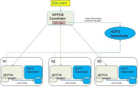
integrated with HDFS, allowing our MPP engine to directly
work on HDFS data and avoid data movement from HDFS
to the FI-MPPDB storage. This approach provides a seam-
less solution between MPPDB and HDFS with better SQL
performance than Transwarp Inceptor, and stronger ACID
support than Cloudera Impala. The HDFS support was
added to the FI-MPPDB in 2016 and successfully adopted
by many of our customers. As a result, FI-MPPDB became
part of Huawei FusionInsight product in 2016.
   In 2017, we announced our first version of FI-MPPDB on
Huawei public cloud, a.k.a. LibrA. Based on our customers’
feedbacks on our cloud offering, the top requirements are 1)
system availability, 2) auto tuning, 3) support querying large   Figure 1: FusionInsight MPPDB System High-level
and diversified data models on the cloud, and 4) best utilize    Architecture
modern hardware for achieving high performance over cost
ratio.
   First, system availability requires that FI-MPPDB should      troduce our cost based approach in JIT compilation in this
be able to add more nodes (elasticity) or go through an up-      paper.
grade with minimal impact on customer workloads. This               The rest of this paper is organized as follows. Section
is critical for large systems with petabytes of data that can    2 presents an overview of the FI-MPPDB architecture fol-
take hours or even days to migrate and re-balance during         lowed by the technical description of the four major direc-
system expansion. Similarly, system upgrade can also take        tions discussed above. Our experimental results are pre-
hours to finish and make the system unavailable for the          sented in section 3, which show the efficiency of our online
end user. These requirements are addressed by our recent         expansion solution, the benefit of auto tuning, the effective-
features online expansion and online upgrade which greatly       ness of the co-location strategy of SQLonHDFS, and the per-
minimize the impact of system expansion and software up-         formance gain from the JIT generated code. Related work is
grades. Due to the space limitation, we will only cover online   discussed in Section 4 which compares our approaches with
expansion in this paper.                                         other industry leaders in the four cloud key areas. Finally,
   Second, DBMS auto tuning minimizes the need for man-          we conclude our paper in section 5 and discuss future work.
ual tuning by system DBAs. For cloud deployment, such
tuning can be complex and costly with the elasticity of the      2.    TECHNICAL DETAILS
system and the access to heterogeneous data sources. Au-           In this section, we first give an overview of FI-MPPDB,
tonomous database from Oracle [13] emphasizes self man-          and then we present our solutions to the four top customer
aging and auto tuning capabilities, an indication that cloud     requirements described in section 1.
providers are paying great attention to this area. We have
been working on automatic query performance tuning through       2.1       System Overview
runtime feedbacks augmented by machine learning.
                                                                    FI-MPPDB is designed to scale linearly to hundreds of
   Third, our cloud customers now have huge amount of data
                                                                 physical machines and to handle a wide spectrum of interac-
in various formats stored in Huawei cloud storage systems,
                                                                 tive analytics. Figure 1 illustrates the high level logical sys-
which are similar to S3 and EBS in AWS. Recently, the
                                                                 tem architecture. Database data are partitioned and stored
notion of Data Lake becomes popular which allows data re-
                                                                 in many data nodes which fulfill local ACID properties.
siding inside cloud storage to be directly queried without
                                                                 Cross-partition consistency is maintained by using two phase
the need to move them into data warehouse through ETL.
                                                                 commit and global transaction management. FI-MPPDB
AWS Spectrum [3] and Athena [1] are recent products that
                                                                 supports both row and columnar storage formats. Our vec-
provide this functionality. Our product provides SQL on
                                                                 torized execution engine is equipped with latest SIMD in-
Hadoop (SQLonHadoop) support (a.k.a. ELK in FusionIn-
                                                                 structions for fine-grained parallelism. Query planning and
sight) which was successfully used by many of our customers.
                                                                 execution are optimized for large scale parallel processing
   Fourth, modern computer systems have increasingly larger
                                                                 across hundreds of servers. They exchange data on-demand
main memory, allowing the working set of modern database
                                                                 from each other and execute the query in parallel.
management systems to reside in the main memory. With
                                                                    Our innovative distributed transaction management (GTM-
the adoption of fast IO devices such as SSD, slow disk ac-
                                                                 lite) distinguishes transactions accessing data of a single
cesses are largely avoided. Therefore, the CPU cost of query
                                                                 partition from those of multiple partitions. Single-partition
execution becomes more critical in modern database sys-
                                                                 transactions get speed-up by avoiding acquiring centralized
tems. The demand from cloud database customers on high
                                                                 transaction ID and global snapshot. GTM-lite supports
performance/cost ratio requires us to fully utilize the great
                                                                 READ COMMITTED isolation level and can scale out FI-
power provided by modern hardware. An attractive ap-
                                                                 MPPDB’s throughput manifold for single-partition heavy
proach for fast query processing is just-in-time (JIT) compi-
                                                                 workloads.
lation of incoming queries in the database execution engine.
By producing query-specific machine code at runtime, the           2.1.1    Communication
overhead of traditional interpretation can be reduced. The
                                                                   Using TCP protocol, the data communication requires a
effectiveness of JIT compiled query execution also depends
                                                                 huge number of concurrent network connections. The maxi-
on the trade-off between the cost of JIT compilation and
                                                                 mum concurrent connections will increase very quickly with
the performance gain from the compiled code. We will in-
                                                                 larger clusters, higher numbers of concurrent queries, and

                                                            1823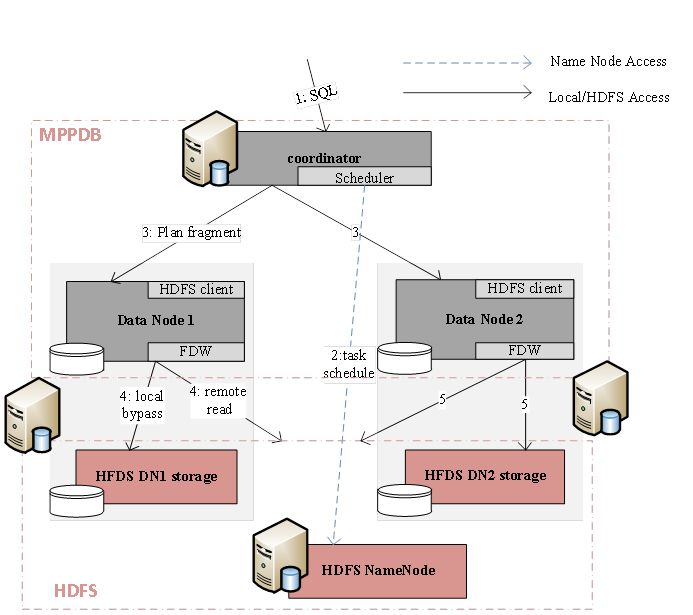
more complex queries requiring data exchange. For exam-             queries such as its application name. The controller evalu-
ple, the number of concurrent connections on one physical           ates queries and dynamically makes decisions on execution
host can easily go up to the scale of one million given a           based on the query’s resource demands (i.e., costs) and the
cluster of 1000 data nodes, 100 concurrent queries, and an          system’s available resources (i.e., capacity). A query starts
average of 10 data exchange operators per query (1000 *             executing if its estimated cost is not greater than the sys-
100 * 10 = 1,000,000). To overcome this challenge, we de-           tem’s available capacity. Otherwise, the query is queued.
signed a unique communication service infrastructure where          Resource bookkeeping and feedback mechanisms are used
each data exchange communication pair between a consumer            in keeping tracking of the system’s available capacity. The
and a producer is considered a virtual or logical connection.       queued queries are de-queued and sent to the execution en-
Logical connections between a given pair of nodes share one         gine when the system’s capacity becomes sufficient.
physical connection. By virtualizing the data exchange con-
nections with shared physical connections, the total number         2.2         Online Expansion
of physical connections on a physical host system is signifi-          Modern massively parallel processing database manage-
cantly reduced. We chose SCTP (Stream Control Transmis-             ment systems (MPPDB) scale out by partitioning and dis-
sion Protocol) as the transport layer protocol to leverage its      tributing data to servers and running individual transactions
built-in stream mechanism. SCTP offers reliable message-            in parallel. MPPDB can enlarge its storage and computa-
based transportation and allows up to 65535 streams to              tion capacity by adding more servers. One of the important
share one SCTP connection. In addition, SCTP can sup-               problems in such scale-out operation is how to distribute
port out-of-band flow control with better behavior control          data to newly added servers. Typically, the distribution
and fairness. All those features match the requirements of          approach uses certain algorithms (such as hash functions,
our design of logical connections and simplify the implemen-        modulo, or round-robin) to compute a value from one col-
tation compared to the customized multiplexing mechanism.           umn (called distribution column in a table). This value is
                                                                    used to determine which server (or database instance) stores
2.1.2    High Availability and Replication                          the corresponding record. The result of those algorithms de-
   It is always a challenge to achieve high availability of         pends on the number of servers (or database instances) in
database service across a large scale server fleet. Such sys-       the cluster. Adding new servers makes those algorithms in-
tem may encounter hardware failures so as to considerably           valid. A data re-distribution based on the number of servers,
impact service availability. FI-MPPDB utilizes primary-             including newly added ones, is needed to restore the consis-
secondary model and synchronous replication. The amount             tency between distribution algorithms’ result and the actual
of data stored in data warehouses are normally huge, up to          location of records. In addition, hash distribution may be
hundreds of TB or even PB, so saving storage usage is a crit-       subjected to data skew where one or more servers are as-
ical way to lower overall cost. A data copy is stored in pri-       signed significantly more data, causing them to run out of
mary and secondary data nodes, respectively. In addition,           space or computing resource. In such cases, one can choose a
a dummy data node maintains a log-only copy to increase             different hashing function, re-compute the distribution map,
availability when secondary data nodes fail. Introducing            and move data around to eliminate the skew and balance the
the dummy data node solves two problems in synchronous              load.
replication and secondary data node catch-up. First, when
secondary data nodes crash, primary data nodes can exe-                 2.2.1    Solution Overview
cute bulkload or DML operations because log can still be               A naive implementation of redistribution is to take the ta-
synchronously replicated to the dummy data nodes. Sec-              ble offline, reorganize the data in place, and move relevant
ond, after recovering from crash, secondary data nodes need         data to newly added nodes. During this process, the table
to catch up with primary data nodes for those updates hap-          cannot be accessed. Alternatively, one can create a shadow
pening when secondary data nodes are down. However, the             table and load it with the data while keeping the original ta-
primary data nodes may have already truncated log, causing          ble open for query. But until the data is redistributed to the
secondary data nodes’ recovery and catch-up to fail. This is        new nodes, the distribution property does not hold among
solved by dummy data nodes providing the needed log.                the new set of nodes. In order to make the table available
                                                                    for query during the redistribution process, one choice is to
2.1.3    Workload Management                                        change table distribution property from hash to random as
  The performance of analytical query processing is often           done in Greenplum [20]. Such an approach allows the data
sensitive to available system resources. FI-MPPDB depends           to be queried, but the query performance is degraded since
on a workload manager to control the number of concur-              data locality information is lost and collocated joins are not
rently running queries. The workload manager optimizes              possible. In addition, data modification operations (such as
system throughput while avoiding the slow-down caused by            IUD) are blocked on the table during redistribution, causing
queries competing for system resources.                             interruption to user workloads for extended period of time.
  The workload manager consists of three main components:              For our solution, we use the shadow table approach for re-
resource pools, workload groups, and a controller. Resource         distribution. But instead of making the table read-only, we
pools are used for allocating shared system resources, such         modify the storage property of the original table to append-
as memory and disk I/O, to queries running in the system,           only mode and prevent the recycling of the storage space.
and for setting various execution thresholds that determine         This gives us an easy way to identify the new records added
how the queries are allowed to execute. All queries run in a        to the table (called append-delta) during data redistribu-
resource pool, and the workload group is used for assigning         tion. Additionally we create a temporary table to store the
the arriving queries to a resource pool. Workload groups are        keys (rowid) of deleted records (called delete-delta). After
used to identify arriving queries through the source of the         the existing data has been redistributed, we lock down the

                                                                 1824
table, reapply the append-delta, and then delete-delta on
the shadow table. To facilitate the application of delete-
delta, the shadow table is created with additional column
that stores the rowid from the original table. This way we
can join the shadow table with delete-delta table to apply
the delete-delta.
Our approach offers the following advantages
• Our solution allows DML operations including insert,
delete, and update while the table is being redistributed.
• Our method of redistribution of a table can be con-
figured to progress in small batches. Each batch can
be done quickly to minimize load increase to the sys-
tem. Each unit is done as a transaction and the whole
redistribution can be suspended and resumed between Figure 2: Example of Redistribution Phases
tables.
• Our method requires only one scan of data in the orig- of its original position during the data redistribution pro-
inal table for the redistribution. This improves the cess. In step 4, a temporary table delete-delta D is created
overall redistribution performance. The only addi- to keep track of the original tuple keys of deleted records.
tional scan of data is done on the shadow table when Since the space in the original table is not reused after the
delete-delta is being applied. redistribution has begun, the tuple key can uniquely iden-
tify a version of a record, allowing us to apply the deletions
• Our method can also be used for cluster downsizing in the new table later on.
without any changes. In both cases, extra space on In steps 5 through 7 we start rounds of redistribution of
each member of the new cluster is needed to store the records from T, one segment at a time. In step 5, we get a
temporary shadow table. The total size of the tempo- snapshot and start to scan a segment of the table, move all
rary shadow table is the same as the size of the original visible records to S, distribute them into a new set of nodes
table. according to the new distribution property (new node group
and/or new hash function), and record the unique original
2.2.2 Core Algorithm
tuple key from the original table in the hidden column of the
Algorithm 1 illustrates the algorithm to execute the redis- new table (explained in step one). In step 6, we apply the
tribution while still allowing normal DML operation on the deletion in this segment happened during the redistribution
table. of the segment by deleting the records in the new table us-
ing the original-tuple-key stored in D. D is reset after it is
Algorithm 1 Algorithm Redistribution DML applied and this phase is committed in step 7.
1: Create a shadow table S with the same schema as the In step 8, we iterate over steps 5 through 7 until the re-
original table T to be redistributed maining data in T is small enough (based on some system
2: Mark T as append only threshold). Step 9 starts the last phase of the redistribu-
3: Disable garbage collection on T tion by locking T, redistributing the remaining data in T
4: Create a delete-delta table D for deletes on T the same way as steps 5-6. This is followed by renaming
5: Redistribute a segment of T into S. the new table S to the original table T in step 10. Step 11
6: Apply D on S and reset D when finished. commits the changes. Finally, we rebuild the indexes on T
7: Commit the change. in step 12.
8: Repeat steps 5-7 until the remaining records in T is Figure 2 illustrates the redistribution process from step 5-
smaller than a threshold 9 using an example with 3 iterations. In this example, T1 is
9: Lock the original table. Redistribute the remaining in- the original table, and T1 tmp is the shadow table with the
sert and delete delta, just as in step 5 and 6. same schema as T1. All three iterations apply both insert
10: Switch the T with S in the catalog. and delete delta changes introduced by Insert, Update and
11: Commit the changes. Delete (IUD) operations of T1 onto T1 tmp while still taking
12: Rebuild indexes IUDs requests against T1. The last iteration which has small
set of delta changes locks on both tables exclusively in a brief
In Algorithm 1, steps 1 through 4 prepare the table T for moment to redistribute the remaining insert and delete delta
redistribution. In step 1, we create a shadow table S with the as described in step 9.
same schema as T plus a hidden column (original tuple key)
to store the original tuple key of records moved from T. In- 2.3 Auto Tuning in Query Optimizer
dexes on S are disabled during this phase until all redistri- Our MPPDB optimizer is based on Postgresql optimizer
bution is done. In step 2, we mark T as append-only and with fundamental enhancements to support complex OLAP
disable reuse of its freed space. With this conversion, inserts workloads. We briefly describe the main architectural changes
to T will be appended to the end of T, deletions are handled in our optimizer. First, our optimizer is re-engineered to
by marking the deleted record, and updates on the T are in- be MPP aware that can build MPP plans and apply cost
ternally converted to deletions followed by inserts. In step based optimizations that account for the cost of data ex-
3, we disable the garbage collection on T to keep records change. Second, the optimizer is generalized to support
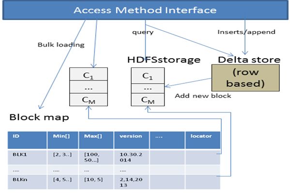
1825predicate (if any), and input description. Obviously, the use
of steps statistics is done opportunistically by the optimizer.
If no relevant information can be found at the plan store,
the optimizer proceeds with its own estimates. Our initial
proof of concept for statistics learning is done for scan and
join steps. We call this approach selectivity matching.
In addition to exact matches with previously stored pred-
icates, auto tuning can be applied to similar predicates as
well. We can gather predicate selectivity feedbacks in a
Figure 3: Statistics Learning Architecture special cache (separate from the plan store cache described
above) and use it to estimate selectivity for similar condi-
tions. Many machine or statistical learning algorithms can
be used for this purpose. We call this second learning tech-
planning and cost based optimizations for vector executions
nique similarity selectivity and we also call this special case
and multiple file systems including Apache ORC file format.
as predicate cache.
Query rewrite is another major ongoing enhancement to
Our similarity selectivity model is initially applied to com-
our optimizer, including establishing a query rewrite engine
plex predicate like x > y +c where both x and y are columns
and adding additional rewrites which are critical to complex
and c is a constant. Such complex predicates are common
OLAP queries.
with date fields. For example, some of the TPC-H queries in-
The enhancements mentioned above are common in other
volve predicates like l receiptdate > l commitdate+c which
commercial database and big data platforms. We believe
restricts line items that were received late by c days. These
that we are closing the gap with those established prod-
predicates pose a challenge to query optimizers and they are
ucts. In addition, we are working on cutting edge technology
good candidates for our similarity selectivity. The more gen-
based on learning to make our optimizer more competitive.
eral form of these predicates is x > y + c1 and x l commitdate + 10 and
dinality estimation (statistics), which is one of the core com-
l receiptdate l commitdate
Our experience shows that most OLAP workloads are fo-
and l receiptdateIn the following sections, we will discuss our recent im-
provements in these areas.
2.4.2 Advanced Data Collocation and Hash Parti-
tioning
HDFS doesn’t support data collocation through consis-
tent hashing algorithm which is a performance enhancement
technique widely adopted in commercial MPPDB systems
including FI-MPPDB. This means standard database op-
erations such as JOIN, GROUP BY, etc will often require
extra data shuffling among the clusters when performed on
HDFS storage.
There are two kinds of data collocation schemes we con-
sidered:
1. Data collocation between MPPDB data nodes and HDFS
data nodes: this allows MPP data nodes to scan data
in HDFS through short-circuit local read interface where
Figure 4: MPPDB Foreign HDFS Data Architecture higher scan speed can be achieved.
2. Table collocations in HDFS data nodes: tables are par-
1. Our Gauss MPP coordinator receives the query in SQL titioned on HDFS data nodes so that co-located join
format. or group by operations can be performed to reduce
network data shuffle cost.
2. Planner constructs the query plan while Scheduler sched-
ules tasks for each MPP data node according to table When FI-MPPDB writes data to the HDFS system, it
splits information from HDFS name node. can apply consistent hash partition strategy. As illustrated
in Figure 5, FI-MPPDB data nodes are co-located with the
3. Coordinator ships the plan fragments with task-to-
HDFS data nodes, where both local and distributed file sys-
Datanode map to each MPP data node.
tem are presented. Direct local reads on HDFS can be done
4. Each MPP data node reads data in a local-read pre- through the HDFS short-circuit read interface. When we
ferred fashion from HDFS data nodes according to the load data into HDFS through our MPPDB data node, we
plan and task map. use a local descriptor table to record each file’s ownership
within each data node. The descriptor table is shown as
In general, a HDFS directory is mapped into a database the Block Map in Figure 6. The table consists of columns
foreign table which is stored like a native relational table for block id, min/max values for each columns in a block,
in FI-MPPDB. Foreign tables can be defined as partitioned a bitmap for deleted records in that block, and a block lo-
tables. A HDFS partition is normally stored as a HDFS cater. Once the data is distributed to each MPP data node,
directory that contains data sharing the same partition key. it will serialize the incoming data stream into specific PAX
Both of our planner and scheduler can take advantage of this style files such as ORC or Parquet and then write these files
to generate plans that skip irrelevant partitions at run time directly to the HDFS. The file replication is taken care of
to reduce I/O. Furthermore, some popular formats of HDFS by HDFS itself. By default, three copies of the file are writ-
file such as ORC or Parquet embed some level of indexes and ten. According to the file placement policy, one of the copies
synopsis within the file itself. Our planner and execution will be placed in the local machine, which is how the data
engine can leverage this information to push predicates down co-location is achieved.
to file readers in order to further improve query performance. Note with this architecture, the block map dictates what
Other improvements we have done include leveraging our HDFS files a node should access according to data partition
vectorized execution engine for efficient query execution and strategy. It only preserves a logical HDFS locality of the
using dynamic multi-dimension runtime filter from star-join files to their MPP worker nodes. The files in HDFS can be
to further prune partitions and reduce data accessing from moved around by HDFS without notifying the MPP cluster
HDFS storage. due to storage re-balancing or node failures. To reduce the
After its release, our SQLonHDFS feature becomes pop- chance of remote file access, we use a HDFS hint to instruct
ular since our customers can directly query large amount HDFS name node to try its best to preserve the original
of data inside HDFS without using ETL to reprocess and location of specified files.
load data into FI-MPPDB. For further improvements, our
customers make two important requirements: 2.4.3 DML support
1. Data collocation: as SQLonHDFS feature gets used Since HDFS is append-only storage and not optimized for
for more critical analytics workloads, customers want reading or manipulating small chucks of data, DML opera-
better performance through data collocation. tions on HDFS can be complex and inefficient. We adopt
a hybrid architecture to support DML operations by com-
2. DML/ACID support: as most of our customers mi- bining a write optimized row format of our MPPDB with
grate from commercial relational data warehouses where a read optimized PAX format in HDFS. DML support ad-
DML and ACID property are maintained, they expect dresses our customer’s requirement of performing occasional
similar functionalities from our system. DML operations on data in HDFS cluster with strong ACID
1827pilation can be extended further to cover more compiler op-
timizations, such as loop unrolling, function in-lining, con-
stant propagation, and vectorization etc. In addition, some
frequently used database functions can be replaced by hard-
ware instructions. For example, CRC32 instruction in x86
hardware can be used as a hash function in various opera-
tors (hash join, hash aggregation), and the hardware over-
flow flag can replace the software code for integer overflow
check.
JIT compiled execution may not always be better than the
standard code interpretation approach. This could be the
case for small data sets where the overhead of JIT compi-
lation is more than the execution speedup. Also, additional
optimizations can be applied on the JIT compiled code. Ex-
amples of such optimizations include function in-lining, loop
unrolling, constant propagation, and vectorization. Such op-
timizations also have a trade-off between the optimization
Figure 5: MPPDB Native HDFS Table Architecture overhead and the speedup they provide. We tackle these
trade-offs by making an intelligent decision among these
three possibilities: (1) use interpreted code without JIT code
generation, (2) JIT code generation without additional op-
timizations (3) JIT code generation with additional code
optimizations.
For a specific query, the cost model (for intelligent deci-
sion making) chooses no code generation if the data size of
the query is small and the performance gain from the gen-
erated code is less than the JIT compilation cost. If the
workload size is large enough, the cost model will choose
the optimal method to generate the most cost effective code
based on the data size and the cost of JIT compilation. Our
cost model is based on the formula (1) below to estimate
the performance gains by applying a specific method of JIT
compiled execution on a specific function or a piece of code.
Figure 6: Native HDFS Table Representation
P = (T1 − T2 ) × N − TJIT cost (1)
property. The visibility of block map determines the visi- In the formula (1) shown above, T1 is the cost of one time
bility of the rows in a block. Specifically, we store inserted execution on the original code, T2 the cost of one time ex-
rows first in a row-based delta table. Only after the delta ecution on the JIT compiled code, N the data size of the
table reaches certain size, it will then be converted and writ- workload, TJIT cost the JIT compilation cost, and P the per-
ten into the HDFS as read optimized PAX format. For the formance gain. The estimation of execution cost is similar
delete operation, there are two scenarios: 1) if a deleted row to the cost model applied in the database optimizer. The
is found in the local delta table, it can be deleted from there JIT compilation cost is estimated according to the size of
immediately; 2) if the deleted row is found in a PAX file, the generated code. Our experiment results show that the
we mark the row deleted in the corresponding bitmap of the actual JIT compilation cost is proportional to the size of the
block map. In this way, we avoid physically rewriting the generated code.
whole file on HDFS before a delete commits. Compaction For a specific query, according to the cost model, the per-
can be done later to physically re-construct the data based formance gain is linearly proportional to the data size of
on the visibility information recorded in the block map when workloads. Suppose, we have two methods of JIT compiled
there are enough rows deleted. An update operation is sim- execution for this query, the formula (2) below illustrates
ply a delete of the existing rows followed by an insert of new how to choose different methods of JIT compiled execution
rows into the delta table. The access interfaces are illus- according to different size of workloads. If the workload size
trated in Figure 6. is not larger than N1 , we do not apply the JIT compiled
execution on this query. If the workload size is between N1
2.5 Intelligent JIT Compiled Execution and N2 , we apply the method with less optimizations and
In our FI-MPPDB, we designed and implemented the less JIT compilation cost. If the workload size is larger than
Just-In-Time (JIT) compiled query execution using LLVM N2 , we apply the method with more optimizations and more
compiler (for short we just refer to it as JIT) infrastructure. JIT compilation cost to achieve better performance.
The JIT compiled code targets CPU intensive operators in
our query execution engine. Our goal is to produce JIT com- 0
(x ≤ N1 ),
piled code with less instructions, less branches, less function P = a1 x + b1 (N1 < x ≤ N2 ), (2)
calls, and less memory access compared with the previous
a x + b
approach of interpreted operator execution. The JIT com- 2 2 (x > N2 ).
1828In the following, we use two queries extracted from real
customer use cases to illustrate how our cost model chooses
the optimal method of JIT compiled execution. Without
loss of generality, these methods of code generation and the
cost model can be applied to many other operators of execu-
tion engine in a database system, for example, IN expression,
CASE WHEN expression, and other aggregation functions
etc.
4-SUM query: SELECT SUM(C1), ... , SUM(C4) FROM
table;
48-SUM query: SELECT SUM(C1), ... , SUM(C48) FROM
table;
For each of the above two queries, we have two meth-
ods of code generation to apply JIT compiled execution. In
the first method, we applied various optimizations includ-
ing loop unrolling, function in-lining, and more code spe-
cialization, to generate the code. In the second method, we
generate the code without optimization. The first method
generates more efficient code but consumes more time to Figure 7: TPC-DS 1000x Query and IUD Workload
produce. The second method has less optimized code but with Online Expansion
requires less time to make compared to the first method.
Our experiment results in section 3.5 show that our cost
model picks the optimal choice between these two options Next, we compare online expansion performance to show
for the two queries. the effect of scheduling the expansion order of tables in bar
e and d. For simplicity, we only executed query workload
3. EXPERIMENTAL RESULTS (no IUD) during online expansion time. Bar d is the elapsed
time for query workload during online expansion with ran-
In this section, we present and discuss experimental re-
dom scheduling which does the table redistribution in ran-
sults of our work in the four areas described in section 2.
dom order. Smart scheduling (bar e) on the other hand
3.1 Online Expansion orders the tables for redistribution according to the order
of tables in the query workload. The smart order basically
Our online expansion tests start with a cluster of 3 phys-
tried to minimize the interaction between the redistribution
ical machines, each of which has 516GB system memory,
and workload to speed up both processes. Comparing the
Intel Xeon CPU E7-4890 v2 @ 2.80 Ghz with 120 cores, and
result from e with that in bar d, a schedule considering the
SSD driver. The actual expansion tests add 3 more physical
access pattern improves data redistribution performance by
machines with the same configuration. We thought OLAP
roughly 2X, and improves the query performance by about
was more appropriate for our test and we decided to use
20%.
the TPC-DS in our test. We loaded the cluster with TPC-
DS data with scale factor 1000 (1 Terabyte) and we ran all 3.2 Auto Tuning in Query Optimizer
the 99 TPC-DS queries. We also used the TPC-DS data
We prototyped capturing execution plans and re-using
maintenance tests for inserts, updates, and deletes (IUDs).
them automatically by our optimizer. We conducted our
Each transaction of IUD modifies or inserts an average of
testing on a 8-nodes cluster running FI-MPPDB. Each node
500-1000 rows. We used a total of 5 threads running on the
is a Huawei 2288 HDP server with dual Intel Xeon eight-
cluster: one for online redistribution, one for queries, and
core processors at 2.7GHz, 96GB of RAM and 2.7 TB of disk
three for IUDs.
running with CentOS 6.6. We loaded the cluster with 1 Ter-
Figure 7 captures the results of our online expansion tests.
abyte of TPC-H data with two variants of the lineitem and
We have conducted two major tests. The first test is cov-
orders tables. The first variant has both tables hash par-
ered by the first 3 bars in Figure 7 (bars a, b and c). Bar a
titioned on orderkey to facilitate co-located joins between
is the total elapsed time for customer application workload
them. The other variant has the lineitem table hash par-
(including query and IUD operations) during online expan-
titioned on part key and the orders table hash partitioned
sion using our new online expansion method. Bar b and c
on customer key. This variant is used to test the impact of
are the total elapsed time for the same workload but using
selectivity on network cost.
offline expansion method at different points of time. In b,
The next three subsections cover three tests that aim at
the workload is executed at the old cluster first followed by
testing the impact of inaccurate predicate selectivity for ta-
the offline cluster expansion, while c is the opposite where
ble scans. The three experiments are: wrong choice of hash
the expansion is followed by workload execution. The total
table source in hash joins, unnecessary data movement for
elapsed time using our new online expansion (bar a) is a lot
parallel execution plans, and insufficient number of hash
better than the workload first then offline expansion (bar b)
buckets for hash aggregation. The experiments are based
and close to the method of offline expansion first and then
on a query shown below.
running workload (bar c). Note that the result in bar a is
actually a lot better than those in bar c because it has a s e l e c t o o r d e r p r i o r i t y , count ( ∗ ) as c t
better response time since user requests can be processed from l i n e i t e m , o r d e r s
during the expansion. The cost of online expansion is more where l o r d e r k e y=o o r d e r k e y and
than offline expansion which is expected. l r e c e i p t d a t e l c o m m i t d a t e + date ‘:?’ ;
1829Table 1: Comparison of actual and estimated selectivity for late line items predicate
Predicate Description Predicate Actual Selectivity Estimated Selectivity
line items received l receiptdata > l commitdata + 60 15% 33%
more than 60 days late
line items received more l receiptdata > l commitdata + 120 0.0005% 33%
than 120 days late
line items received l receiptdata ≤ l commitdata − 40 8% 33%
40 days early or less
line items received l receiptdata ≤ l commitdata − 80 0.05% 33%
80 days early or less
Note , i s ‘’ f o r l a t e l i n e items
The above query checks late/early line items based on dif-
ference between receipt and committed dates. The predicate
that checks how early/late a line item like l receiptdata >
l commitdata + 120 poses a challenge to query optimizers
and we thought it is a good example of statistics learning.
Most query optimizers use a default selectivity for such pred-
icates (MPPDB use 1/3 as the default selectivity). Table 1
shows actual and estimated selectivity of these predicates
for different values of being late or early.
Figure 8: Performance comparison on early/late re-
3.2.1 Hash join plan problem ceived orders query (in min.)
We ran the early/late line items query using the differ-
ent options for being early/late per the entries in Table 1.
Figure 8 illustrates the performance difference between the
orders table, or replicate lineitem table. Note that big data
current optimizer and our prototype for the early/late order
engines always have these three options for joining tables
query. The join in this query does not require shuffling data
since HDFS data are distributed using round robin and thus
since both tables are co-located on the join key (this is the
join children are not co-located on the join key.
first variant). Assuming hash join is the best join method
The query optimizer chose the shuffle option (among the
in this case, choosing the right hash table build is the most
three above) which involves the least amount of data move-
critical aspect of the plan for this query. The orders table
ment to reduce the network cost. The standard optimizer
is 1/4 of the lineitem table, and the current optimizer as-
elects to re-partition both lineitem and orders tables (op-
sumes 1/3 of the rows in lineitem satisfying the early/late
tion 1 above) for all variations of the early/late line item
predicate. This leads the current optimizer to choose the
query. This is the case since the size estimates of both ta-
orders table as the hash build side for all the variations of
bles are close. This plan is coincidentally the best plan for
the query.
three cases of the variations (line 1,2 and 5 in Table 1) of
The inaccurate estimate of the selectivity did not have an
the early/late line items query. However, this plan is not
effect on the plan for line items with relatively close values of
optimal for the other cases where the filtered lineitem is
l receiptdate and l commitdate (line 1,2 and 5 in Table 1).
smaller than orders table. Figure 9 captures the run-time
The reason is that the orders table is still smaller than the
for this case of early/late line items query. The performance
lineitem table for those cases and placing it in the hash table
difference is more compelling than those in Figure 8 since
is a good execution plan. The other cases of too late/early
it includes both the extra data shuffle and the original hash
(lines 3, 4, 6 and 7 in Table 1) have the opposite effect with
table plan problem.
smaller lineitem table, and in those cases the auto tuning
estimate outperformed the standard estimate.
3.2.3 Insufficient hash buckets for hash aggregation
3.2.2 Unnecessary data shuffle For the third and last test, we ran the official TPC-H Q4.
Inaccurate predicate selectivity could also have an impact As explained in the introduction section, The performance of
on the amount of data shuffled in MPP join plans which the plan of TPC-H is sensitive to the size of the hash aggre-
are typically used to place matching join keys on the same gation table set by the optimizer. The hash table size is set
node. This problem is tested by running the same early/late based on the number of distinct values for l orderkey which
line items query discussed in the previous section on the is impacted by selectivity of l receiptdate > l commitdate.
second variant of lineitem and orders tables where they are The standard default selectivity of “1/3” produced under-
not co-located on the join key. With this data partitioning, estimates on number of rows and thus a lower estimate on
the optimizer has three options to co-locate the join keys the number of distinct values which misled the optimizer
and perform the join in parallel on the data nodes. These to use less hash buckets than needed for the hash aggregate
options are: re-partition both tables on orderkey, replicate step. This resulted in almost 2X slowdown (53 seconds vs 28
1830Table 3: Specific Selectivity Estimation Error for
Early/Late Line Items
Cache c = -80 c = -40 c = 60 c = 120
Size selectivity 8% 15% 0.0005%
= 0.05%
100 0.2% 0% 0% 0.05%
50 0.7% -0.2% 3.8% 0%
25 5.0% 0.8% -4.6% 0.8%
Figure 9: Performance comparison on early/late re- Table 4: Selectivity Estimation Error for Normal
ceived orders query with shuffle (in min.) Line Items
Cache Size Cache Hits KNN Error
Table 2: Selectivity Estimation Error for Early/Late 100 4 3.1%
Line Items 50 1 4.0%
Cache Size Cache Hits KNN Error 25 1 6.0%
100 218 1.2%
50 118 2.0%
25 65 3.6% former predicate is modeled with a single parameter (how
early/late) in the predicate cache while the latter by two.
Overall, our experiments show that the KNN approach is
seconds) compared to the optimal number of hash buckets highly accurate in selectivity estimation: the absolute esti-
computed using our prototype. mate errors are no more than 4% for single parameter case
and no more than 6% for two parameters case. The details
3.2.4 Join Selectivity Experiment are described below.
The previous sub-sections cover in details three scenarios We use the lineitem table from the TPC-H which has 6M
where selectivity learning for table scans has significant im- rows. We focus on the early items satisfying the condition
pact on query performance. We also did one experiment for l receiptdate ≤ l commitdate − c days, and late items satis-
learning join predicates selectivity. The experiment is based fying the condition l receiptdate > l commitdate + c days.
on the query shown below. We can combine early and late items and model them with
a single predicate cache: the parameter is the difference be-
s e l e c t count ( ∗ )
tween l receiptdate and l commitdate with early items hav-
from l i n e i t e m , o r d e r s , customer
ing negative differences (c) and late items positive ones. We
where l o r d e r k e y=o o r d e r k e y and
randomly generate 500 predicates with c between −80 and
l s h i p d a t e >= o o r d e r d a t e +
120. The average selectivity of such predicates is found to
i n t e r v a l ‘121 days’
be 18%. For each predicate, we find its actual selectivity,
and o c u s t k e y=c c u s t k e y
use the KNN to estimate its selectivity, and compute the
and c a c c t b a l between
estimation error. We repeat this experiment with different
( s e l e c t 0 . 9 ∗min( c a c c t b a l ) from customer ) and
cache sizes of 100, 50, and 25. The average absolute estima-
( s e l e c t 0 . 9 ∗max( c a c c t b a l ) from customer )
tion errors for the 500 tests are shown in Table 2. We can see
group by c mktsegment ;
that larger caches provide better results but even with the
The query above finds those line items that took 121 days smallest cache, the error is still pretty small (3.6%). Note
or more to process and handle. The query excludes top and that the cache is seeded with a random c before it is used
bottom 10% customers in terms of their account balance. for selectivity estimation. When the cache is full the LRU
The query runs in 425 seconds with our current optimizer. policy is used. The predicates only have 200 possible val-
The execution plan is not optimal and it joins customer and ues for c so the cache hits are relatively high. For example,
orders first and then joins the result to line item table. The with a size of 25, the cache stores 1/8 of the possible values
root cause is that the optimizer uses 33% as the default and there are 65 cache hits among the 500 tests. To see the
selectivity for l shipdate ≥ o orderdate + interval0 121day 0 KNN in use, we test it with specific predicates from Table 1
instead of the actual 1% selectivity. Using our learning com- where c is in {−80, −40, 60, 120}. The estimated selectivity
ponent, we get the optimal plan which runs in 44 seconds errors (negatives are under-estimation) are shown in Table
with more than 9X improvement. 3. Overall, the estimation is pretty accurate with the biggest
errors at about 5% with a cache size of 25.
3.3 Cache Model-based Selectivity Estimation To demonstrate the effectiveness of KNN with 2 param-
In this section, we demonstrate the use of KNN for our eters, we also do experiments for the normal line items:
similarity selectivity approach. We tried varying K and predicate l receiptdate between l commitdate − c1 days and
found that K = 5 worked well for various cases. In this ap- l commitdate + c2 days are generated with two uniformly
proach, the selectivity of a predicate is estimated to be the distributed variables 1 ≤ c1 ≤ 80 and 1 ≤ c2 ≤ 120. The
average selectivity from its 5 nearest neighbors in the pred- average selectivity of such predicates is 67%. The results are
icate cache. We pick two predicates for experiment: one shown in Table 4. The estimation errors are pretty small rel-
for early/late items and the other for normal items. The ative to the average selectivity of 67%. Note that the cache
1831Figure 10: Performance comparison Figure 11: Speedups on different queries by apply-
ing different methods of code generation
hits are much less as there are 9600 possible combinations
of c1 and c2. With the smallest cache size of 25, which is
only 0.3% of possible combinations with a single cache hit,
the estimation error is only 6%.
As stated above, we start using the cache for selectivity
estimation when it only has a single predicate. This is a
valid approach as the single selectivity is likely to gives us a
estimate for similar predicates. This is probably better than
a default selectivity such as 33%. Our experiments show
that the cache estimation errors stabilize quickly as more
feedbacks are available. In practice, we can allow the user
to control the use of the cache for unseen conditions, e.g.,
use the cache for prediction only when it has entries more
than a threshold. The cache can also keep the estimation Figure 12: Performance gains from JIT compiled
errors, and the use of it can be shut down if the errors are execution on TPC-H
excessively large for a certain number of estimations. This
can happen when there are very frequent updates on the running with CentOS 6.6. We tested our intelligent JIT
predicate columns. compilation strategy on the two queries mentioned in section
3.4 Advanced Data Collocation Performance 2.5: 4-SUM and 48-SUM queries. The queries are extracted
Improvement for SQLonHDFS from actual Huawei use cases, and the table has about 100
million rows. Figure 11 shows the results for these queries.
As described in section 2.4, we enhanced our SQLonHDFS The optimal solution for 4-SUM is the first method of code
solution by applying the FI-MPPDB hash distribution strat- generation with LLVM post-IR optimization while the speed
egy to the HDFS tables and leverage upon the data distri- up is better for 48-SUM query without LLVM post-IR opti-
bution property through SQL optimizer to produce efficient mizations. For both queries, our intelligent decision making
plans. We conducted performance testing on an 8-node clus- system (cost model) selected the optimal solution.
ter running FI-MPPDB with the HDFS storage to demon- Our more comprehensive test is based on the TPC-H
strate the performance improvement. Each node is a Huawei workload with 10X data. Figure 12 shows that our JIT
2288 HDP server with dual Intel Xeon eight-core proces- compiled execution approach outperforms the previous ap-
sors at 2.7GHz, 96GB of RAM and 2.7 TB of disk running proach with no code generation. The average performance
with CentOS 6.6. We loaded the cluster with 1 terabyte of improvement on the 22 queries is 29% (geometric mean).
TPC-H data in two flavors: one data set is randomly dis-
tributed while the other data set is hash distributed based
on distribution columns. In the second case, the distribution 4. RELATED WORK
columns are carefully selected for each TPC-H table accord- In this section, we discuss some work related to the four
ing to the popular join columns in order to avoid expensive major technical areas presented in this paper.
data shuffling for the workload. Online Expansion We could not find in literature about
Figure 10 shows the results running the 22 TPC-H queries online cluster expansion over large data warehouses with
on the two data sets with different distribution properties. concurrent DML operations without downtime. The clos-
By taking advantage of data collocation, hash distribution est known work is about online expansion in Greenplum
clearly provides much better performance by lowering the [20] which supports redistributing data efficiently without
network shuffling cost. It obtains over 30% improvement noticeable downtime while guaranteeing transaction consis-
(geometric mean) in query elapsed time. tency. However, their solution blocks DML operations dur-
ing online expansion because their data redistribution com-
3.5 Intelligent JIT Compiled Execution mand uses exclusive table locks during expansion. Amazon
Our experiment setup is a single node cluster with one Redshift [2] also provides cluster resizing operation. How-
coordinator and two data nodes, and the server node is a ever, it puts the old cluster in read-only mode while a new
Huawei 2288 HDP server with dual Intel Xeon eight-core cluster is being provisioned and populated. Snowflake [15]
processors at 2.7GHz, 96GB of RAM and 2.7 TB of disk takes a different approach in cluster expansion that allows
1832users to dynamically resize the warehouse with predefined Intelligent JIT Compiled Execution CPU cost of
size such as SMALL , MEDIUM, and LARGE etc. Carlos et query execution is becoming more critical in modern database
al. [21] provide a design tool, FINDER, that optimizes data systems. To improve CPU performance, more and more
placement decisions for a database schema with respect to database systems (especially data warehouse and big data
a given query workload. systems) adopt JIT compiled query execution. Amazon
Auto Tuning Early known work on database auto tun- Redshift [2] and MemSQL (prior to V5) [12] transform an
ing include Database Tuning Advisor [18] from Microsoft incoming query into C/C++ program, and then compile
SQL Server and LEO [30] from IBM DB2 system. LEO is a the generated C/C++ program to executable code. The
learning based optimizer that focuses on predicate selectiv- compiled code is cached to save compilation cost for fu-
ities and column correlation but does not cover the general ture execution of the query since the cost of compilation
case of operator selectivities. Our learning approach is sim- on a C/C++ program is usually high [27]. In comparison,
pler and more general since it captures actual and estimates the LLVM JIT compilation cost is much lower so there is
for all steps and re-use the information for exact or similar no need to cache the compiled code. Cloudera Impala [24]
steps in future query planning. and Hyper system [27] apply JIT compiled execution us-
Using machine learning in query optimization, performance ing LLVM compiler infrastructure, but they only have a
modeling, and system tuning has increasingly drawn atten- primitive cost model to decide whether applying the JIT
tion to the database community [32, 19]. Recent works [22, compilation or not. Spark 2.0’s [16] Tungsten engine emits
25, 26] use machine learning methods to estimate cardinality optimized bytecode at run time that collapses an incoming
for various database operators. The approach using machine query into a single function. VectorWise database system
learning technique is promising as it allows the system to [23] applies the JIT compiled execution as well as the vector-
learn the data distribution and then estimate the selectivity ized execution for analytical database workloads on modern
or cardinality. In contrast, the traditional statistics based CPUs. Our FI-MPPDB adopts JIT compiled execution us-
selectivity estimation has its limitation on the information ing LLVM compiler infrastructure to intelligently generate
a system can store and use. However, we need to carefully the optimal code based on our cost model.
assess the benefits of adopting machine learning based ap-
proaches in commercial database query optimizer as they
may require significant system architecture changes. For
5. FUTURE WORK AND CONCLUSION
example, [25, 26] use neural networks to model selectivity In this paper, we have presented four recent technical ad-
functions which require significant training to approximate vancements to provide online expansion, auto tuning, het-
the functions. In addition, the training set takes consider- erogeneous query capability and intelligent JIT compiled ex-
able system resources to generate. In comparison, our sim- ecutions in FI-MPPDB. It is a challenging task to build
ilarity selectivity approach uses query feedbacks where no a highly available, performant and autonomous enterprise
training is necessary. Our approach is close to [22] where data analytics platform for both on-premise and on the cloud.
KNN is used. We keep it simple by gathering similar feed- Due to space limit, we briefly mention two of our future
backs into a single predicate cache. The one to one mapping works. First, cloud storage service such as AWS S3, Mi-
between predicate types and predicate caches makes it easy crosoft Azure Storage, as well as Huawei cloud’s OBS (Ob-
to integrate the approach into optimizer architecture. ject Block Storage) have been widely used. Users often want
SQL on HDFS Apache HAWQ [8] was originally devel- to directly query data from the centralized cloud storage
oped out of Pivotal Greenplum database [10], a database without ETLing them into their data warehouse. Based
management system for big data analytics. HAWQ was on customer feedback, we are currently working on provid-
open sourced a few years ago and currently incubated within ing SQLonOBS feature in our cloud data warehouse service
Apache community. With its MPP architecture and robust based on the similar idea of SQLonHadoop described in this
SQL engine from Greenplum, HAWQ implements advanced paper. Second, auto tuning database performance using ma-
access library to HDFS and YARN to provide high perfor- chine learning based techniques is just starting but gaining
mance to HDFS and external storage system, such as HBase heavy momentum. In addition to selectivity learning, we
[4]. SQL Server PDW allows users to manage and query data plan to look into parameter learning, where key parameters
stored inside a Hadoop cluster using the SQL query language the query optimizer uses to make decisions can be auto-
[29]. In addition, it supports indices for data stored in HDFS matically learned. We also plan to explore other machine
for efficient query processing [28]. learning techniques.
With the success of AWS Redshift [2], Amazon recently
announced Spectrum [3]. One of the most attractive features 6. ACKNOWLEDGMENT
of Spectrum is its ability to directly query over many open
We thank Qingqing Zhou, Gene Zhang and Ben Yang for
data formats including ORC [6], Parquet [7] and CSV. FI-
building solid foundation for FI-MPPDB, and Harry Li, Lei
MPPDB also supports ORC and CSV formats, while neither
Liu, Mason Sharp and other former team members for their
Redshift nor Spectrum supports HDFS.
contribution to this project while they worked at Huawei
In the Hadoop ecosystem, Hive [5] and Impala [24] are
America Research Center. We also thank Huawei head-
popular systems. SparkSQL [16] starts with the focus on
quarter team for turning these technologies into a successful
Hadoop, then expands its scope onto S3 of AWS. While
product on the market.
they are popular in open source and Hadoop community, the
lack of SQL compatibility and an advanced query optimizer
make it harder to enter enterprise BI markets. In contrast, 7. REFERENCES
our SQLonHDFS system can run all 99 TPC-DS queries
[1] Amazon Athena - Amazon.
without modification and achieve good performance.
https://aws.amazon.com/athena/.
1833You can also read