Eddy covariance flux errors due to random and systematic timing errors during data acquisition - Biogeosciences
←
→
Page content transcription
If your browser does not render page correctly, please read the page content below
Biogeosciences, 15, 5473–5487, 2018
https://doi.org/10.5194/bg-15-5473-2018
© Author(s) 2018. This work is distributed under
the Creative Commons Attribution 4.0 License.

Eddy covariance flux errors due to random and systematic timing
errors during data acquisition
Gerardo Fratini1 , Simone Sabbatini2 , Kevin Ediger1 , Brad Riensche1 , George Burba1,3 , Giacomo Nicolini2 ,
Domenico Vitale2 , and Dario Papale2,4
1 LI-COR  Biosciences Inc., Lincoln, Nebraska 68504, USA
2 Dipartimento per la Innovazione nei sistemi Biologici, Agroalimentari e Forestali – DIBAF, Università degli
Studi della Tuscia, Viterbo, 01100, Italy
3 R. B. Daugherty Water for Food Institute, School of Natural Resources, University of Nebraska,

Lincoln, Nebraska 68583, USA
4 Centro Euro-Mediterraneo sui Cambiamenti Climatici – CMCC, Lecce, 73100, Italy

Correspondence: Gerardo Fratini (gerardo.fratini@licor.com)

Received: 9 April 2018 – Discussion started: 23 April 2018
Revised: 26 July 2018 – Accepted: 18 August 2018 – Published: 14 September 2018

Abstract. Modern eddy covariance (EC) systems collect            nor characterized a posteriori. Therefore, it is important to
high-frequency data (10–20 Hz) via digital outputs of instru-    test the ability of traditional and prospective EC data logging
ments. This is an important evolution with respect to the tra-   systems to assure the required synchronicity and propose a
ditional and widely used mixed analog/digital systems, as        procedure to implement such a test relying on readily avail-
fully digital systems help overcome the traditional limita-      able equipment.
tions of transmission reliability, data quality, and complete-
ness of the datasets.
   However, fully digital acquisition introduces a new prob-
lem for guaranteeing data synchronicity when the clocks          1   Introduction
of the involved devices themselves cannot be synchronized,
which is often the case with instruments providing data via      Eddy covariance (EC) is the most direct and defensible tech-
serial or Ethernet connectivity in a streaming mode. In this     nique to measure atmosphere–biosphere exchange fluxes of
paper, we suggest that, when assembling EC systems “in-          energy and matter to date (e.g., see Aubinet et al., 2000,
house”, aspects related to timing issues need to be carefully    2012; Baldocchi et al., 2001). The method is based on the
considered to avoid significant flux biases.                     Navier–Stokes equations for mass and momentum conserva-
   By means of a simulation study, we found that, in most        tion and relies on simplifying assumptions to describe the
cases, random timing errors can safely be neglected, as they     vertical turbulent flux in terms of the covariance of the verti-
do not impact fluxes significantly. At the same time, sys-       cal wind component (w) and of the scalar of interest.
tematic timing errors potentially arising in asynchronous           Calculating EC fluxes of a gaseous species requires col-
systems can effectively act as filters leading to significant    lecting synchronous data of w and of the concentration c of
flux underestimations, as large as 10 %, by means of at-         the gas, which is typically performed using a 3-D ultrasonic
tenuation of high-frequency flux contributions. We charac-       anemometer and a gas analyzer operating at suitable frequen-
terized the transfer function of such “filters” as a function    cies of 10 to 20 Hz. After proper data treatment and time
of the error magnitude and found cutoff frequencies as low       alignment, the covariance of the two time series is calculated,
as 1 Hz, implying that synchronization errors can dominate       from which the flux is derived (e.g., Foken et al., 2012). In
high-frequency attenuations in open- and enclosed-path EC        this context, synchronicity means that w and c values for any
systems. In most cases, such timing errors neither be detected   given timestamp (i.e., the data that are multiplied together in
                                                                 the covariance) describe the properties of the same air parcel.

Published by Copernicus Publications on behalf of the European Geosciences Union.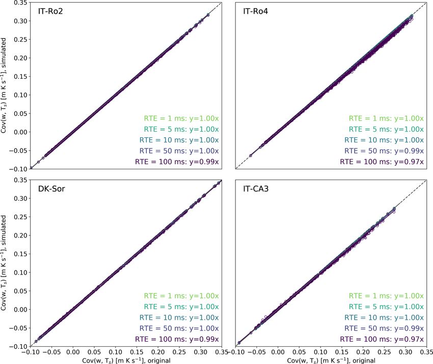
5474                                                                          G. Fratini et al.: Eddy covariance timing errors

   Regardless of the level of integration and physical configu-     Plüss, 2010). For example, analog signals from the gas ana-
ration of the instruments within an EC system, wind and con-        lyzer were sent to an interface unit responsible for digitizing
centration data are measured by two different instruments, an       the data before merging it with anemometric data, itself com-
anemometer relying on the speed of sound measurements be-           ing from an A/D (analog/digital) converter into the interface
tween transducer pairs, and a gas analyzer relying on the light     unit, typically from a sonic anemometer-thermometer (SAT).
transformation measurements in the sampling path. In addi-          More recently, specular solutions, with the analog data from
tion, data collection is performed by means of a variety of         the SAT sent to an interface unit residing in the gas analyzer
more or less engineered data acquisition systems. Delays in         system, became available and were widely adopted. With
the data flows, digital clock drifts, required separation of the    both of these approaches, the data were presented to the user
measuring devices, and artifacts in the data acquisition strat-     for the flux calculation as single files with wind and gas time
egy can lead to poor synchronicity, i.e., to misalignments of       series merged and synchronized by the interface unit.
the time series, such that w and c values assigned to a given          Analog data output allows the data to easily cross clock
timestamp refer to properties of fully or partially different air   domains. The clock that is used to sample the original signal
parcels. If not addressed, such misalignments can lead to sig-      does not need to be synchronized to the clock that samples
nificant flux errors of both a random and systematic nature.        the analog output. This makes it very convenient to merge
   Commercial solutions implementing sound engineering              data from systems with unsynchronized clocks and risks of
practices do exist for well-established EC measurements of          misalignments are limited to small random errors that, as we
CO2 and H2 O fluxes to assure a sufficient level of data syn-       will see later, have no significant effects on fluxes.
chronicity as per the requirements of the EC method, for               However, collecting data in analog form has several limi-
a select few anemometer–analyzer pairs. However, most of            tations and risks. First, the number of analog channels avail-
such solutions are not scalable to other hardware models or         able either as outputs from the instruments or as inputs to
gas species because the required instrumentation does not           the interface unit is typically limited to four or six, which
necessarily support the same connectivity technology and            dramatically reduces the number of variables that can be col-
specifications. Therefore, it is generally very challenging,        lected. In fact, historic EC raw datasets are comprised of six
for example, to simply replace a gas analyzer with another          or maximum seven variables: the three wind components (u,
one from another manufacturer and keep the same synchro-            v, w), the sonic temperature (Ts ), and the concentration of
nization performance. Furthermore, it is customary for many         the gases of interest (c, traditionally CO2 and H2 O); more
research groups to assemble EC systems “in-house”, espe-            rarely, a diagnostic variable for the anemometric data was
cially when addressing gas species that have not been pop-          also collected. Critical information such as the full diagnos-
ular enough to grow strong commercial interest. Typically,          tics of both instruments and their status (e.g., the temperature
in these systems, data collection is performed with industrial      and pressure in the gas analyzer cell or the signal strength)
data loggers or computers via serial or Ethernet connectivity,      or the original raw measurement (speed of sound, raw data
using custom-built logging software. In such cases, it is par-      counts etc.) are not collected in most analog systems, limit-
ticularly important to verify that various types of data mis-       ing the means for quality screening and limiting the possi-
alignment are not being introduced by the data logging sys-         bility of future recomputation of the most fundamental raw
tem and data collection strategy to assure minimal or no bias       measurements. Another problem with analog data collection
in resulting fluxes.                                                is that signals are subject to degradation due to dissipation,
   In this paper, we discuss the types and sources of misalign-     electromagnetic noise, and ageing of cables and connectors,
ment that can arise in poorly designed fully digital EC sys-        which reduces the quality of collected data (Barnes, 1987).
tems and quantify their effects on resulting fluxes. In con-        In addition, although all raw measurements are analog in na-
junction with site-specific characteristics, such as the typi-      ture, they are typically immediately digitized (native digital
cal co-spectral shapes, this information can help design ap-        format provided by the manufacturer) and then – in the case
propriate data collection scheme for EC systems assembled           of analog data collection – they are re-converted to analog,
“in-house”. Users of most commercially available industrial-        sent to the interface unit and there converted back to digi-
grade EC systems can generally assume their systems to not          tal; these A/D–D/A conversions potentially degrade the sig-
be affected by significant timing errors, although this can and     nal adding noise and dampening high-frequency signal com-
should be verified case by case. We also propose a strategy         ponents (Eugster and Plüss, 2010). For these reasons, analog
for evaluating prospective EC data collection systems from          connectivity should nowadays be avoided whenever possible
the point of view of data synchronicity before they are used        in favor of fully digital solutions.
in routine field activities.                                           In fully digital EC acquisition systems, both data streams
                                                                    are collected in their respective native digital format, i.e.,
1.1    Analog vs. digital EC systems                                without additional A/D conversions other than those imple-
                                                                    mented by the manufacturer to provide digital outputs. Fully
Traditionally, a combination of analog and digital transmis-        digital systems largely or completely overcome both prob-
sion systems has been used to collect EC data (Eugster and          lems with mixed analog/digital systems, using more robust

Biogeosciences, 15, 5473–5487, 2018                                                      www.biogeosciences.net/15/5473/2018/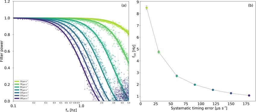
G. Fratini et al.: Eddy covariance timing errors                                                                              5475

and less corruptible data transmission protocols, and provid-      As for commercial solutions, LI-COR provides industrial-
ing the possibility of collecting all variables available from     grade EC systems based on the SmartFlux® system, that can
the individual instrument. However, combining digital data         accommodate a wide variety of instrumentation using the
streams from different instruments brings new challenges,          data-streaming approach.
most notably with respect to data synchronization. While              However, collecting data in streaming mode exposes the
moving between clock domains is trivial in an analog sys-          risk of introducing significant timing errors, because of the
tem, it can be much more challenging with digital data when        number of asynchronous digital clocks involved.
the involved clocks can be completely asynchronous to each            Digital clocks are electronic oscillator circuits that use the
other.                                                             mechanical resonance of a vibrating crystal of piezoelec-
                                                                   tric material to create an electrical signal with a precise fre-
1.2   The problem of clock synchronization in digital              quency, which is then used to keep track of time. The number
      systems                                                      and quality of clocks involved in an EC system vary with the
                                                                   data collection strategy and technology. In systems based on
Different strategies exist for collecting data digitally. First,   data triggering or polling, there is only one critical clock (the
instruments can perform the measurements according to their        one responsible for the timing of the triggering or polling
own scheduler or a trigger. In the scheduler case, data can        signal); therefore, there is no significant risk of introducing
then be collected by polling the instrument for the latest         systematic timing misalignments between data from different
available data (polling mode) or by keeping an open chan-          instruments (see later). With these systems, the risk is limited
nel where data are streamed (streaming mode). In the trigger       to random and/or constant misalignments. As we will see
case, data are usually made available after a fixed or some-       later, random or constant misalignments do not entail large
what variable delay to the logging device. This delay is due       errors. For this reason, in the remainder of this section we
to the acquisition time and could also include a delay due         consider in more detail the situation with systems based on
to filtering. However, the timestamp for the acquired data is      data streaming.
assigned based on the occurrence of the trigger, therefore re-        In such systems the potentially relevant clocks are, in gen-
moving any timing error due to that delay. All modes have          eral, the following.
advantages and disadvantages. As described later, triggering
and polling modes are less susceptible to timing errors, but         – The sampling clocks of the sensing instruments (the
they require the instrumentation to be designed for the partic-        SAT and the gas analyzer in a typical EC system), re-
ular triggering or polling system adopted. They are therefore          sponsible for sampling data at the prescribed rate with
best suited for EC systems built with all components from the          sufficient precision and accuracy;
same manufacturer. For the same reason, such systems are
                                                                     – For systems that transmit data serially (RS-232 or RS-
commonly not flexible enough to accommodate third-party
                                                                       485), the serial clock of the same sensing instrument,
instrumentation. EC systems commercialized by Campbell
                                                                       which may or may not be correlated to its sampling
Scientific Inc. (Logan, UT, USA; “CSI” hereafter) are exam-
                                                                       clock;
ples of integrated systems using a data triggering strategy to
collect data from instruments designed ad hoc. Data com-             – The clocks of the logging device(s) (data logger, PC,
munication in these systems is realized via the synchronous            etc.), responsible for attaching a timestamp to the data.
devices for measurement (SDM) protocol (or its evolutions),            If a single logging device is used, this is usually also
which is a CSI proprietary protocol, implemented only in               responsible for merging data streams from the different
CSI instruments and some CO2 /H2 O gas analyzers by LI-                instruments; in case dedicated logging systems are used
COR Biosciences Inc. (Lincoln, NE, USA; “LI-COR” here-                 for different instruments, merging is performed in post-
after). By contrast, most instrumentation available for fast           processing and the clocks of the different loggers must,
wind and gas measurements only provide data transmission               therefore, be aligned sufficiently frequently (e.g., every
options in streaming mode. As a consequence, most data                 second, using a GPS signal).
logging solutions developed by the scientific community or
by commercial entities are designed to handle data provided        Typical open digital communication protocols used for EC
in streaming mode and are therefore flexible to accommo-           instruments with data-streaming instrumentation are serial
date a wide variety of instrumentation. Examples of such           (RS-232, RS-485) and packet-based data protocols (Ether-
logging systems developed by the community are PC-based            net). In devices that transmit data via serial communication,
software such as Huskerflux (https://github.com/Flux-Dave/         such as SATs, there are no means to synchronize the sam-
HuskerFlux, last access: 26 June 2018), EddyMeas (Kolle            pling clock of the device to that of the data logger. With such
and Rebmann, 2007), EdiSol (EdiSol User Guide V0.39b               devices, the best that can be done is to assign a timestamp
https://epic.awi.de/29686/1/Mon2005d.pdf, last access: 26          after transmission, based on the clock of the data logger (this
June 2018), or the already referenced system proposed by           last step should be performed carefully to avoid large inac-
Eugster and Plüss (2010) for EC measurement of methane.            curacies due to serial port latencies, especially in PC-based

www.biogeosciences.net/15/5473/2018/                                                      Biogeosciences, 15, 5473–5487, 2018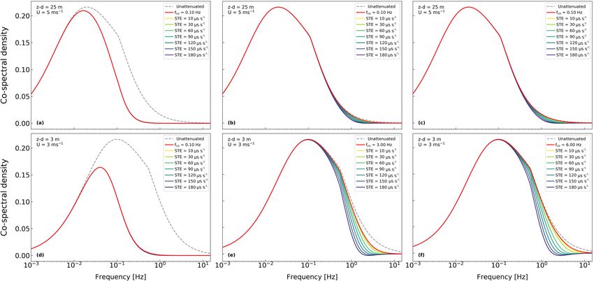
5476                                                                            G. Fratini et al.: Eddy covariance timing errors

systems). In addition, devices implementing serial commu-
nication have an asynchronous clock that drives those pro-
tocols (e.g., Dobkin et al., 2010). If this clock is correlated
with the device’s sampling clock, the receiving data logger
can – at least in principle – reconstruct the sampling clock.
However, in devices that do not correlate sampling and serial
clocks (such as those that output data in a software thread that
is independent of an acquisition thread), the system sched-
uler then determines when data are transmitted, thereby com-
pletely isolating the serial clock from the sampling clock and
making it impossible for the data logger to reconstruct the
sampling clock.
   Packet-based data communications such as Ethernet even
further isolate the sampling clock from the transmission
clock. In devices using this protocol, it is therefore impos-
sible to reconstruct a sampling clock. However, for Ethernet-
based systems additional protocols are available, such as
Network Time Protocol (NTP) or Precision Time Protocol
(PTP), to actually synchronize all system clocks. The syn-
chronized system clocks then allow the data to be correctly
timestamped before transmission, eliminating any synchro-
nization issue, provided that downstream software can align
the various data streams based on their timestamps (e.g.,          Figure 1. Schematic of the three types of misalignments common
Mahmood et al., 2014).                                             in EC data. Given a reference time series (e.g., w, blue), the ideal
                                                                   paired gas concentration time series is perfectly aligned (green).
1.3    Types of timing errors                                      The three red time series exemplify (from left to right): a constant
                                                                   offset (time lag), random variations around the perfect alignment
In typical EC data acquisition setups, time series collected       (random error), and a systematically larger time step (systematic er-
by different instruments can show three distinct types of mis-     ror). Real data are typically affected by a mix of all error types in
alignments (Fig. 1).                                               varying amounts.

  – Time lags: these are constant offsets in otherwise per-
    fectly aligned time series. They can be the result of con-             slightly longer or shorter than the nominal one for time
    stant electronic delays or of fixed delays due to digital              spans on the order of the flux averaging interval. Again,
    signal processing. More frequently, they result from a                 in EC we are only concerned with systematic relative
    physical separation of the sampling volumes or from the                errors, for identical errors in the two concerned instru-
    delay due to the time needed for the passage of air in a               ments would entail no misalignment and hence no flux
    sampling line.                                                         bias.

  – Random timing errors (RTEs in the following): occur            Instances of each type of misalignment can, and typically
    when the timestamps assigned to the data differ from the       will, be present at the same time to various degrees.
    exact time dictated by the nominal sampling frequency,
    and such differences are randomly distributed so that,         1.4     Sources of misalignment and their effects on time
    on average, the actual frequency is equal to the nominal               series
    one. In practice, in the EC context, it is more useful to
    consider the random differences in the timestamps as-          1.4.1     Spatial separation between sampling volumes
    signed to data from one instrument with respect to that
    of the paired instrument. In fact, in the hypothetical case    In a SAT, the sampling volume is the volume of air between
    in which the two instruments would have the exact same         the upper and lower sets of transducers. Similarly, in an open-
    sequence of random errors, that would not introduce any        path gas analyzer such as the LI-7500 CO2/H2O analyzer
    misalignment and hence no flux bias.                           and the LI-7700 CH4 analyzer (LI-COR Biosciences Inc.,
                                                                   Lincoln, NE, USA), the sampling volume is the volume of
  – Systematic timing errors (STEs): occur when the times-         air between the upper and lower mirrors. In a closed- or
    tamps assigned to the data differ from the exact time          enclosed-path gas analyzer such as the LI-7000, the LI-7200
    dictated by the nominal sampling frequency, and such           (LI-COR Biosciences Inc.), and the EC155 (Campbell Sci-
    differences are systematic, e.g., the actual time step is      entific Inc., Logan, UT, USA), instead, the sampling volume

Biogeosciences, 15, 5473–5487, 2018                                                       www.biogeosciences.net/15/5473/2018/
G. Fratini et al.: Eddy covariance timing errors                                                                             5477

can be identified with the volume of the intake device, e.g., a    Frequency drift
rain cup.
   Even in the hypothetical situation of perfectly synchro-        The oscillation frequency of a clock varies with tempera-
nized timestamps for wind and gas data, if the respective          ture, leading to drifts of the measured time and hence to
instruments’ sampling volumes have to be spatially sepa-           STEs. The drift of a clock can be expressed as the amount
rated to avoid presently intractable flow distortion issues in     of time gained (or lost) as a result of the drift per unit of
the anemometer, as is notably the case with open-path setups       time, with suitable units being µs s−1 . For example, a drift
(see, for example, Wyngaard, 1988; Frank et al., 2016; Grare       of −30 µs s−1 means that a clock accumulates 30 µs of de-
et al., 2016; Horst et al., 2016; and Huq et al., 2017), the       lay per second, or about 2.6 s over the course of 1 day (2.6 =
corresponding time series will be affected by misalignment,        30 ×10−6 ×(24 × 60 × 60)). The dependence of a crystal os-
possibly to varying degrees. Indeed, assuming the validity of      cillation frequency on temperature varies, even dramatically,
Taylor’s hypothesis of frozen turbulence, wind and concen-         with the type and angle of crystal cut and can be modeled
tration data will be affected by a time lag (the time air takes    as quadratic (BT, CT, DT cuts) or cubic (AT cuts) (Hewlett
to travel between the two sampling volumes), which will be         Packard, 1997). Figure 2 shows exemplary drift curves for
further modulated by wind intensity and direction. Addition-       different crystal cuts. Typically, the nominal frequency (e.g.,
ally, modification of turbulence structure intervening while       32 kHz) is specified at 20 or 25 ◦ C. Apart from that tempera-
air parcels transit through the dislocated instrument volumes      ture, the frequency can vary, for example, according to (for a
may introduce further uncertainty in flux estimates (Cheng et      BT cut):
al., 2017). In the case of co-located sensors (e.g., Hydra-IV,
                                                                   f − f0
CEH; IRGASON, Campbell Scientific Inc.) this problem is                   = −α(T − T0 )2 × 10⁻⁶ ,                              (1)
not present but is replaced by the flow distortion issues men-       f0
tioned above and not addressed in the present study.
                                                                   where f0 = f (T0 = 25 ◦ C) and typical values of α range be-
1.4.2   Spatial separation between measuring volumes               tween 0.035 and 0.040.
                                                                      Clocks in EC systems can be exposed to large variations
In a SAT, the sampling volume coincides with the measur-           in temperature (day–night, seasonal cycles). Because we are
ing volume, i.e., wind velocity is measured exactly where          concerned with relative drifts, we are interested in differ-
it is sampled. The same is true for open-path gas analyzers.       ences in the temperatures experienced by the instruments’
However, closed- and enclosed-path analyzers take the sam-         sampling/logging clock as well as with differences in their
pled air into a measuring cell via a sampling line that can be     temperature responses. Clocks experiencing similar temper-
anywhere between 0.5 and 50 m long, with its inlet usually         atures and with similar temperature responses, would mini-
placed very close to the SAT sampling volume. This implies         mize relative drift. On the contrary, clocks with opposite re-
a delay of the time series of gas concentrations with respect      sponses to temperature will result in relative drifts that are
to the wind time series. Such a delay can be more or less          close to the sum of the individual drifts, e.g., in the case of
constant in time depending on the possibility of actively con-     AT-cut crystals with different angles of rotation at relatively
trolling the sampling line flow rate. In systems without flow      high temperatures (i.e., above 30 ◦ C, see Fig. 2)
controllers, the flow rate may vary significantly in response         It is also to be noted that temperature-compensated clocks
to power fluctuations or tube clogging and so would the cor-       do exist, which have accuracies of around ±2 µs s−1 . As we
responding time lags.                                              will show later, such drifts can be safely neglected, as long
                                                                   as clocks are synced sufficiently often (e.g., once a day). For
1.4.3   Clock errors                                               completeness, we note that clock drifts also occur due to the
                                                                   ageing of components. However, the absolute values of typ-
Quartz crystal clocks universally used in electronic devices       ical ageing rates (< 1 µs year−1 ) are of no concern in EC ap-
are subject to two main types of error: periodic jitter and fre-   plications. Because STEs in EC systems are caused primarily
quency drift.                                                      or exclusively by clock drifts, in the rest of the paper we will
                                                                   use the terms STE and drift interchangeably.
Period jitter
                                                                   1.4.4   Further sources of timing errors in digital
Period jitter in clock signals is the random error of the clock            asynchronous systems
with respect to its nominal frequency. It is typically caused by
thermal noise, power supply variations, loading conditions,        Connectivity
device noise, and interference coupled from nearby circuits.
Jitter is a source of RTE in time series.                          Ethernet connectivity available in commercial loggers and
                                                                   industrial PCs (e.g., SmartFlux 2 and 3 by LI-COR Bio-
                                                                   sciences Inc., CR3000 and CR6 by Campbell Scientific Inc.)
                                                                   can be used for data acquisition in EC systems. The acqui-

www.biogeosciences.net/15/5473/2018/                                                      Biogeosciences, 15, 5473–5487, 2018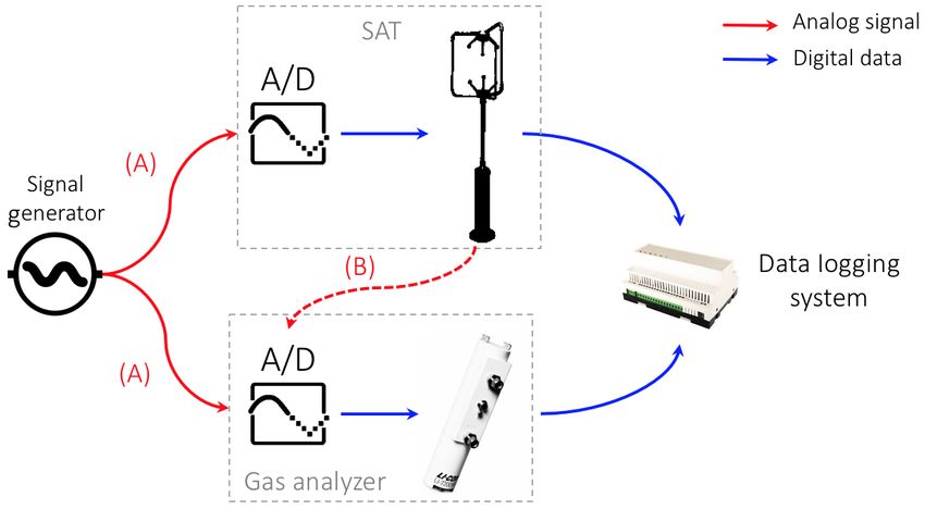
5478                                                                               G. Fratini et al.: Eddy covariance timing errors

Figure 2. Exemplary temperature dependence curves for clocks with AT (a), BT (b), CT (c), and DT (d) cuts. In (a) the three curves refer to
different angles of rotations of the crystal. Reproduced and adjusted from Hewlett Packard (1997).

sition is usually done using the Transmission Control Proto-            20 Hz, concluding that the flux errors are negligible in most
col (TCP), a packet-based protocol specifically designed to             applications.
preserve the accuracy of the data during transmission. TCP,                For completeness, we note that in virtually all EC instru-
however, is not designed to preserve the temporal aspect of             ments the native measurement is time-discrete. For example,
the packets. The TCP receiving system must buffer up pack-              in a nondispersive infrared (NDIR) gas analyzer, the pres-
ets and signal the sender if an error occurs in any packet. This        ence of a rotating filter used to multiplex the desired infrared
can cause packets to even arrive out of order, even though              bands makes the gas concentration measurement frequency
they are always delivered to the application in order. There-           dependent on the wheel rotational frequency, which leads to
fore, TCP-based systems are subject to significant RTEs and,            RTEs. Nonetheless, if the rotational speed is high enough
potentially, to STEs.                                                   (e.g., > 100 Hz), the resulting errors are minimal.
   Serial communication devices typically use a first-in-first-
out (FIFO) policy to buffer data, on both the sending and               1.5   Dealing with timing errors in EC practice
the receiving sides. The FIFO increases the efficiency and
throughput by reducing the number of interrupts the CPU                 The fundamental difference between time lags on one side
has to handle (e.g., Park et al., 2003). Without a FIFO buffer,         and RTE/STE on the other side is that constant time lags can,
the CPU has to interrupt for every data unit. With a FIFO,              at least in principle, be addressed a posteriori during data pro-
the CPU is interrupted only when a FIFO is full, or a pro-              cessing. The topic of correctly estimating and compensating
grammed amount of data is ready. However, the FIFO can                  time lags has long been discussed in the EC literature (Vick-
become a problem on a system where it’s desired to corre-               ers and Mahrt, 1997; Ibrom et al., 2007; Massman and Ibrom,
late the serial clock to the sampling clock. If not properly            2008; Langford et al., 2015), and corresponding algorithms
handled, the FIFO introduces timing jitter on both the trans-           are available in EC processing software. We will therefore
mitter and the receiver, hence inducing RTEs in the system.             not further discuss time lags in this paper.
                                                                           Random and systematic timing errors, instead, are not
Time response                                                           identifiable and therefore it is not possible to correct them.
                                                                        However, their effect on flux estimates, as we will see, can
In a streaming-based system, an instrument with a time re-              become significant. For this reason, the only viable strategy
sponse (irrespective of the supported output rate) slower than          to reduce flux biases is to design the data acquisition system
the sampling rate will lead to RTEs even in the absence of              in a way that prevents or minimizes the possibility of their
any clock errors, because the measurement cannot in general             occurrence.
be performed at the required moment in time. In the general                The focus of this paper is, therefore, the quantification of
case, such an instrument will be oversampled (i.e., the same            flux underestimations as a function of RTE and STE, so as to
measured value will appear multiple times in the final time             derive quantitative specifications for a data acquisition sys-
series). Eugster and Plüss (2010) discuss in detail the con-            tem that minimizes EC flux losses. We further propose a sim-
sequences of such an occurrence with a CH4 gas analyzer                 ple scheme for evaluating existing data acquisition systems
with a time response of 5.7 Hz in a system sampling data at             with respect to data synchronization.

Biogeosciences, 15, 5473–5487, 2018                                                           www.biogeosciences.net/15/5473/2018/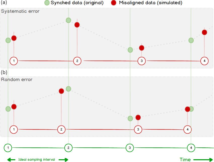
G. Fratini et al.: Eddy covariance timing errors                                                                                       5479

Figure 3. Sketch of the timing error simulation via linear interpolation. Green dots represent original Ts data points, equally spaced at the
prescribed (nominal) time steps. In (b), RTEs are simulated as time steps randomly varying around the nominal value. In (a), STEs are
simulated as a time step larger than the nominal one, whereby the difference between the assigned and correct timestamps always increase
in time.

2     Materials and methods                                              tions intervening between covariance and flux computation,
                                                                         such as spectral corrections and consideration of air density
2.1    Simulation design                                                 fluctuation effects (e.g., Fratini et al., 2012). The simulation
                                                                         study was implemented in the source code of EddyPro v6.2.1
In order to accurately quantify how time-alignment errors                (LI-COR Biosciences Inc, Lincoln, NE; Fratini and Mauder,
affect flux estimates, we performed a simulation study. As               2014).
a reference, we used the covariance estimated from high-                    For the present analysis, we simulated RTEs ranging ±1
frequency data of vertical wind speed (w) and sonic tempera-             to ±100 ms; that is, up to the same order of the sampling
ture (Ts ) which are by definition perfectly synchronized since          interval. As an example, with a simulated ±10 ms RTE us-
they are computed starting from the same raw data (the trave             ing 10 Hz data (nominal time step = 100 ms), simulated time
ling time of sound signals between pairs of transducers in a             steps for Ts varied randomly between 90 and 110 ms, with an
SAT). We also assumed that high-frequency time series are                average of 100 ms. We note that RTEs of 10–100 ms will not
provided at perfectly constant time steps of 0.1 (10 Hz) or              usually be caused by clock jitter, which is typically several
0.05 (20 Hz) seconds. Subsequently, we manipulated the ar-               orders of magnitude smaller but can easily be caused by ac-
ray of timestamps at which the sonic temperature data were               quisition systems based on serial or Ethernet communication
sampled in order to simulate realistic ranges of RTEs and                not specifically designed to collect synchronous time series,
STEs. Values of sonic temperature in correspondence to the               as described above.
new simulated timestamps were estimated by linearly inter-                  For STEs, we simulated relative drifts ranging from 10
polating the closest data points in the original series (Fig. 3).        to 180 µs s−1 (specifically 10, 30, 60, 90, 120, 150, and
   Before calculating covariances, standard EC processing                180 µs s−1 ). For example, to simulate a STE of 60 µs s−1 we
steps were applied such as spike removal (Vickers and Mahrt,             kept the original w time series (time step equal to 100 ms)
1997), tilt correction by the double rotation method (Wilczak            and modified the time step of Ts to be 100.006 ms. This may
et al., 2001), and fluctuation estimation via block-averaging.           seem a negligible difference, which accumulates a difference
Covariance estimates obtained with the new versions of Ts                of 108 ms between w and Ts within 30 minutes and mani-
were then compared with the reference to quantify the effect             fests itself as a difference of one row in the length of the time
of simulated timing errors. Flux biases would be almost iden-            series (i.e., 18 000 value for w and 17 999 for Ts at 10 Hz).
tical to biases in covariances, weakly modulated by correc-

www.biogeosciences.net/15/5473/2018/                                                              Biogeosciences, 15, 5473–5487, 2018
5480 G. Fratini et al.: Eddy covariance timing errors
Similarly, systematic errors of 120 and 180 µs s−1 would lead 25 m tall and the EC system placed at 60 m a.g.l. (Pile-
to two and three row differences, respectively. gaard et al., 2011).
Systematic timing errors such as frequency drifts effec-
tively act as low-pass filters, which can be described by char- – IT-CA3: fast-growing short-rotation coppice of poplar
acterizing their transfer function, provided that the drift is clones planted in 2010, located in Castel d’Asso,
known, as in our simulation. Here, for each 30 min period Viterbo, Italy. The EC tower was installed at the end
and for each STE amount, we calculated an in situ transfer of 2011, and measurements were taken until mid-2015.
function as the frequency-wise ratio of drifted and original The period used for the simulation included 9 months
w-Ts co-spectra: over the period 2012–2015, with a canopy height rang-
ing 0–5.3 m, and the measurement height between 3 and
CO w, TsSTE | fn
5.5 m (Sabbatini et al., 2016).
TFEXP (fn ) = ,
CO (w, T | fn )
2.3 Validation of the simulation design
for STE = [10, . . ., 180] µs s−1 , (2)
Although the proposed simulation design enables the evalu-
where TsSTE (K) is the simulated sonic temperature for ation of resulting errors using readily available EC data, we
each STE value, fn (Hz) is the natural frequency, and note that interpolating data sampled at 10 or 20 Hz frequency
TFEXP (STE|fn ) is the in situ transfer function for STE. We can potentially introduce artifacts (due to the lack of infor-
repeated this calculation for a number of co-spectra ranging mation at higher frequencies) such as, for example, an undue
from 1000 to 2000 (depending on data availability). The en- reduction of the sonic temperature variance, which would re-
semble of all transfer functions so obtained and for each STE sult in artificial reduction of the w-Ts covariance. In order to
amount was then fitted with the following function, which detect any such effects, we preliminarily implemented a val-
was found to reasonably approximate the data obtained for idation procedure, making use of 1 week of sonic data from
all drifts at all sites in the most relevant frequency range a Gill HS-100 (Gill Instruments Ltd., Lymington, UK) col-
(0.01–5 Hz): lected at 100 Hz. The validation involved the following steps:
1 1. Subsampling at 10 Hz and simulating timing errors as
TF(fco |fn ) = (1 + β) α − β, (3)
fn described above, i.e., interpolating starting from the
1+ fco
subsampled data.
where fco (Hz) is the transfer function cutoff frequency and
2. Subsampling at 10 Hz and simulating timing errors by
α and β are fitting parameters whose values were found to
interpolating the original 100 Hz data.
vary very little around α = 2.65 and β = 0.25.
3. Comparing w-Ts covariances obtained in steps 1 and 2.
2.2 Datasets
The timing errors simulated interpolating the original 100 Hz
We performed simulations on four datasets acquired from EC measurements (option 2 above) are much less prone to ar-
sites representative of various ecosystem types and climatic tifacts because interpolation occurs between data that are
regimes and characterized by the different height of measure- 0.01 s apart, an interval too short for any significant flux sig-
ment and height of the canopy: nal to occur. Using this procedure, we could verify that there
– IT-Ro2: a deciduous forest of Turkey Oak (Quercus cer- is no detectable difference between results obtained with 100
ris L.) in Italy. Eddy covariance measurements were and 10 Hz data (not shown), which implies that the inter-
carried out from 2002 to 2013 and the period used for polation procedure is not introducing significant artifacts in
the simulations was May 2013, when the canopy height the estimation of variances and covariances and therefore the
was 15 m and the measurement height 18 m (Rey et al., simulation can be performed with virtually any historic EC
2002). dataset using the available code.
– IT-Ro4: located at about 1 km from IT-Ro2, is a rotation
crop site where EC measurements have been carried out 3 Results and discussion
from 2008 to 2014. Data used for the simulations in-
clude 43 days in 2012 when crimson clover (Trifolium Figure 4 compares covariances w-Ts obtained with increas-
incarnatum L.) was cultivated (maximum canopy height ing amounts of RTE against the reference covariance ob-
60 cm, measurement height of 3.7 m). tained with the original, perfectly synced, time series. Reduc-
tion in covariance estimates is fairly negligible provided that
– DK-Sor: evergreen forest near Sorø, Denmark. EC mea- RTE is of the same order of magnitude of the sampling inter-
surements are performed since 1997: during the period val or less. Largest discrepancies were observed for the IT-
used for the simulation (the entire 2015) the forest was CA3 and IT-Ro4 sites with a covariance underestimation of
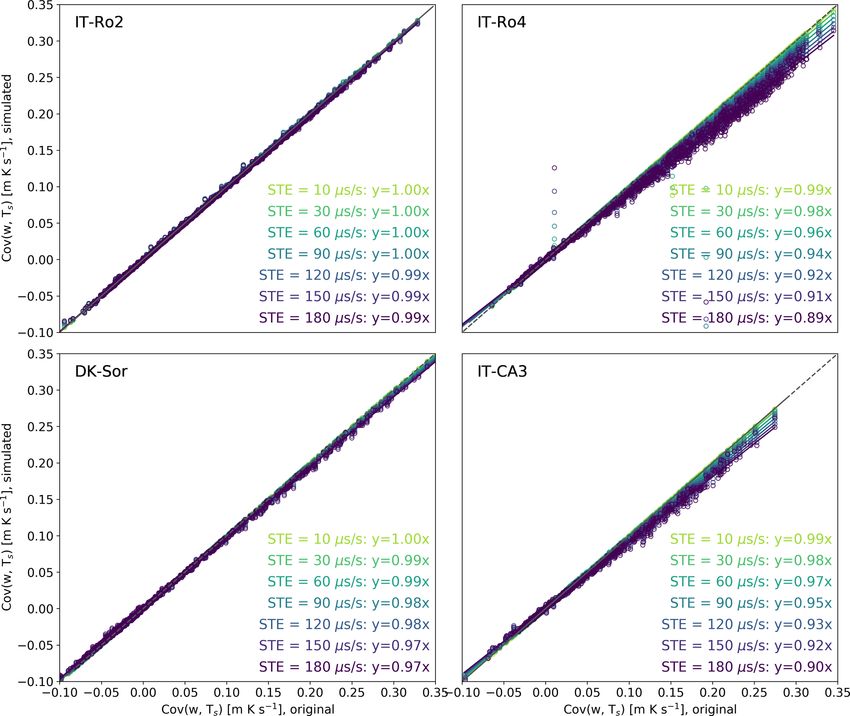
Biogeosciences, 15, 5473–5487, 2018 www.biogeosciences.net/15/5473/2018/G. Fratini et al.: Eddy covariance timing errors 5481 Figure 4. Simulation of RTEs. Covariances w-Ts obtained with a set of simulated random errors of different amplitudes (y axes) are compared to the covariances w-Ts computed with the original time series (x axes), for the four sites. All regressions had an offset equal to zero and r 2 > 0.99. 3 % for RTE of amplitude 100 ms. As mentioned earlier, such The reason is related to the distribution of the flux con- large timing errors are never the result of electronic clock jit- tributions across the frequency domain. The more the flux ter and may instead be caused by a data transmission system co-spectrum is shifted towards higher frequencies, the more not designed for time synchronization, such as TCP. it will be dampened by any given low-pass filter and the Conversely, flux biases induced by systematic timing er- higher the resulting flux bias will be. In other words, sys- rors are both more significant and more variable. Figure 5 tematic timing errors are a source of high-frequency spectral shows that a STE of 60 µs s−1 (1 row of difference in a 30 min losses, not dissimilar to the ones traditionally considered in file with data collected at 10 Hz) can lead to errors anywhere EC (Moncrieff et al., 1997; Massmann, 2000; Ibrom et al., between 0 % and 4 %, increasing to 1 %–8 % for a STE of 2007). Figure 7 depicts the low-pass filtering effects of sev- 120 µs s−1 (2 rows of difference) and to 1 %–11 % for a STE eral STEs as applied to three different hypothetical EC sys- of 180 µs s−1 (3 rows of difference). tems, characterized by different “initial” cutoff frequencies Figure 6a shows an example of the transfer functions de- (caused by other sources of attenuation such as, for exam- rived using the procedure described in Sect. 2.1. The Fig- ple, length of the sampling line) deployed in two contrasting ure refers to the site IT-CA3, but the filters obtained for the scenarios (high vs. low measurement height). It is evidenced other sites had very similar characteristics, as illustrated in that at high measurement heights effects are negligible, ir- Fig. 6b using the mean cutoff frequencies computed for all respective of the “original” cutoff frequency of the system sites at each STE amount: the tight ±3.5σ range merely (a–c). The reason is that the STE filters act on co-spectra that demonstrates that the low-pass filter properties of the STE are shifted to low frequencies and have therefore very low are independent from the data used to derive it, and only vary high-frequency content. At low measurement height, instead, with the error amount. STEs significantly increase spectral losses if the system has Nonetheless, in Fig. 5 we showed how the same STE leads a high initial cutoff frequency (e–f), while if the system as to very different flux underestimations at a different site. For a poor initial spectral response (d), STEs are irrelevant be- example, a systematic error of 180 µs s−1 led to flux biases cause, again, high-frequency co-spectral content is minimal of 1 % and 11 % at IT-Ro2 and IT-Ro4, respectively. to start with. www.biogeosciences.net/15/5473/2018/ Biogeosciences, 15, 5473–5487, 2018
5482                                                                               G. Fratini et al.: Eddy covariance timing errors

Figure 5. Simulation of STE. Covariances w-Ts obtained with a set of simulated systematic errors of different amplitudes (y axes) are
compared to the covariances w-Ts computed with the original time series (x axes), for the four sites. All regressions had an offset equal to
zero and r 2 > 0.98.

Figure 6. Transfer function for the STE at different error amounts, as derived using Eqs. (2) and (3), using data from site IT-CA3 (a). Mean
values and 3.5σ ranges of the transfer function cutoff frequencies across the fours sites, as a function of the error amount (b).

   To put this new source of high-frequency losses in per-              ues are usually found in systems based on open-path setups.
spective quantitatively, we note that for EC systems based              Significant STEs can thus easily become leading sources of
on an enclosed-path gas analyzer (LI-7200), cutoff frequen-             flux biases in modern EC systems deployed at low measure-
cies ranging from 1.1 Hz (for less optimized) up to 7–8 Hz              ment heights and/or very limited spectral losses due to other
(for systems with optimized intake rain cup and heated sam-             causes, with the additional complication that they are hard
pling line) were reported in the literature (e.g., Fratini et al.,      to detect and quantify. In fact, once acquired and stored in
2012; Aubinet et al., 2016; Metzger et al., 2016). Similar val-         files, it is generally not possible to establish whether a drift

Biogeosciences, 15, 5473–5487, 2018                                                           www.biogeosciences.net/15/5473/2018/
G. Fratini et al.: Eddy covariance timing errors                                                                                      5483

Figure 7. Effect of adding artificial STEs to three EC systems characterized by different cutoff frequencies (0.1, 3.0, and 6.0 Hz for d, e,
and f, respectively) and by different measurement height and mean wind speed (from a–c to d–f).

between data streams occurred. Missing lines in one data                Evaluating synchronicity of an EC data acquisition
stream could be either filled in by the data acquisition soft-          system
ware (e.g., by means of the “last observation carried forward”
technique) or could be compensated by dropping one line in
the paired, longer series. In both cases, one would be un-              If both EC instruments can receive analog inputs, a possible
able to detect the problem, which is, however, obviously not            way to evaluate synchronicity in the data logging system is
solved by these solutions, meant only to build a complete               to connect a signal generator to both EC instruments (SAT
rectangular dataset. On the contrary, a mismatch of one or              and gas analyzer) and collect the data via the data logging
two lines in the length of the time series is not necessarily           system in the configuration that would be adopted in normal
the sign of an occurring STE, as it could also be the result            operation (Fig. 8). The result is two replicates of the known
of an imperfect timing in opening/closing a data stream, or             signal data, whose timestamps will in general not be synchro-
some combination of the two factors. For these reasons, it is           nized, in the sense that the same nominal timestamp will be
very difficult, if not practically impossible, to detect STEs,          attached to two different pieces of data. The two datasets can
distinguish them from other timing errors or artifacts, and,            then be compared to calculate the phase difference between
more importantly, to infer the type and amount of error that            the clocks and hence assess RTEs and STEs. For example,
is being introduced in the covariances. The only sign of a po-          a cross correlation of the time series yields the phase differ-
tential timing problem is an attenuated co-spectrum, as eval-           ence. It’s important to test the time series at different time in-
uated with respect to an available reference or model. But              tervals, e.g., 0.5 h for several days, in actual field conditions
from the co-spectra attenuation alone, it is impossible to es-          that undergo significant temperature variations. The two in-
tablish the presence of a timing error and, even more, dis-             struments are synchronized if the cross correlation yields the
entangle it from other sources of attenuation. The only pos-            same result every time. If this constant phase offset (time lag)
sibility is thus to estimate an ensemble spectral correction            is different from zero, this measurement quantifies signal de-
based on co-spectra, which would correct only sources of er-            lays in a system, which can be addressed either by optimizing
rors without the ability to discriminate them, which is less            the data logging system or by taking this offset into account
than ideal (e.g., Ibrom et al., 2007). It is therefore advised to       while setting up the time-lag automatic computation in post-
evaluate the performance of a data acquisition system before            processing. A cross correlation that changes over time, in-
it is put in operation.                                                 stead, is a strong indication of occurring STEs. It is very dif-
                                                                        ficult to anticipate the evolution in time of the phase change
                                                                        as it depends on the clock’s crystal cuts, quality, and temper-
                                                                        ature sensitivity. In general, we may expect a linear trend in
                                                                        the phase if temperatures do not vary strongly (see also later)

www.biogeosciences.net/15/5473/2018/                                                             Biogeosciences, 15, 5473–5487, 2018
5484 G. Fratini et al.: Eddy covariance timing errors Figure 8. Schematic of possible setups to evaluate the ability of a data logging system to synchronize EC data. In setup A the same (known) analog signal (solid red lines) is sent to the analog inputs of the EC instruments where it is digitized. In setup B analog wind data (dashed red line) is sent to the gas analyzer, where it is digitized. In both setups, the two digital data streams are then collected by the data logging system. The clocks involved and how timestamps are attached to data depend on the specifics of the system under consideration. or a trend modulated by a diurnal pattern if temperature plays a role. A simpler (though less controlled) option, in case a signal generator is not accessible, is to use the analog outputs from at least one of the EC instruments. In this case the test in- volves transmitting (at least) one of the analog outputs to the analog input of the companion instrument (e.g., w sent via analog output of the SAT to an analog input channel of the gas analyzer). In this way the raw-data files contain two repli- cates of that variable, each collected according to the timing of the respective instrument: the timestamps of the digital version are logged according to timing of the sending instru- ment (SAT, in the example), while those of its analog version are logged according to the timing of the receiver (gas ana- lyzer). The same cross-correlation analyses described above Figure 9. Evolution of time lags between two replicates of the same can then be performed. variable (u wind component, but identical results were obtained In both versions of the tests, results may be affected by mi- with v and w), one collected with the SAT native digital format and nor RTEs if the various A/D or D/A tasks are not accurately one collected via analog outputs from the SAT. Data were collected synchronized with the measurement and serial output tasks. in two files roughly 70 h long and then split into 30 min chunks for However, such RTEs should not affect the ability to detect the computation of time lags. and quantify occurring STEs. Note also that, in both versions of the test, the way raw data are stored may have a strong impact on how to interpret unit (LI-COR Biosciences Inc.) which was then collected the results. For instance, depending on the specifics of the via a second RS-232 port (indicated with subscript a), us- data acquisition system, collecting a unique file with 3 days ing an industrial-grade PC running Windows XP. Thus, the worth of data or collecting 30 min files for 3 days can provide data logging system under testing was “a Windows PC col- different results, e.g., because the act of closing a file and lecting EC data via RS-232, which was setup to transmit data opening a new one can cause the data streams to be partially in streaming mode”. The two data streams were completely or completely “realigned”. independent to each other, and we attached timestamps to To exemplify the test, we collected about 3 days of 20 Hz the records based on the operating system clock as the data wind data from a SAT (HS-100, Gill Instruments Ltd., were made available from the serial port to the application Lymington, UK) both in native digital format (via a RS-232 collecting the data. We then merged the two datasets based port, indicated with the subscript d in the following) and in on timestamps and split the resulting 3-day file into 30 min. analog format via the A/D of a LI-7550 analyzer interface Finally, we calculated time lags between pairs of homolo- Biogeosciences, 15, 5473–5487, 2018 www.biogeosciences.net/15/5473/2018/
G. Fratini et al.: Eddy covariance timing errors                                                                                   5485

gous variables (e.g., ud vs. ua , but results were identical for   leads to significant relative drifts among the time series,
all anemometric variables), which are shown in Fig. 9. The         which is bound to generate flux underestimations. With mi-
linearity of the data suggests that the system is affected by a    nor ad hoc adjustments, the same testing setup can be used
fairly constant STE of about 50 µs s−1 , as quantified by the      to evaluate any EC data logging system. While evaluation
slope of the line.                                                 of existing systems was beyond the scope of our work and
   Using the same setup, we further collected 2 days of data       we do expect synchronization issues to be more of a risk for
directly stored as 30 min files and again computed time lags       in-house solutions, the proposed testing setup for evaluating
between homologous variables. The acquisition system was           data synchronization applies equally to in-house and to com-
able to realign the two series at the beginning of each half       mercial solutions and we do invite researchers and compa-
hour resetting the time lag between them to roughly zero.          nies to test their systems.
Nevertheless, calculating time lags on overlapping 5 min pe-          With this in mind, we recommend the scientific commu-
riods, we found that within each half-hourly period the time       nity to promote collaboration and synergy among manufac-
lags increased by 0.05 s (32 % of the times) and of 0.1 s (68 %    turers of EC equipment, technological solutions that guaran-
of the times), which again indicates an STE ranging from 30        tee sufficient synchronicity do exist – such as Ethernet con-
to 60 µs s−1 which, as shown above (Fig. 5), can lead to de-       nectivity deploying the PTP protocol – but, in order to be uti-
tectable flux biases. We stress that the system used in this       lized, they require all instrumentation to be compatible with
experiment was not optimized for data acquisition and the          those technologies, which is not yet the case.
aim was solely that of evaluating the proposed test.                  A final note on the data collected until now and largely
                                                                   shared and used in publications. As stated above, it is im-
                                                                   possible to detect the presence of a synchronization issue on
4   Conclusions                                                    archived dataset. However, fully digital acquisition in stream-
                                                                   ing mode started to be largely adopted only recently and this
Undoubtedly, modern EC systems should log high-frequency           limits the potential impact of the issue on historical data. In
data in a native digital format, so as to collect all possi-       addition, as also explained in the results, the effect of a STE
ble measurement, diagnostic, and status information from           acts as a spectral loss and hence it may be (at least partially)
each instrument and assure the creation of robust, self-           compensated for and corrected by in situ spectral corrections
documented datasets, which are essential to the long-term          based on co-spectra.
research goals of climate and greenhouse gas science.
   Commercial data acquisition solutions exist, that one can
legitimately expect to ensure a proper data synchronization,       Code availability. The source code for performing the simulation
such as the SmartFlux® system by LI-COR or the SDM-                is available in the following public repository: https://github.com/
based system by CSI. There also exist applications developed       geryatejina/ec_timing_errors_simulation (Fratini, 2018).
by research institutions that specifically address the synchro-
nization issue. In all these cases it is, however, possible to
test the synchronization in order to confirm the expected per-     Competing interests. The authors declare that they have no conflict
                                                                   of interest.
formances.
   When dealing with novel gas species, however, assem-
bling EC systems from instrumentation that is not necessarily
                                                                   Author contributions. GF and DP conceived and designed the
designed to be integrated is often the only choice available to
                                                                   work. GF carried out all the simulations and data analysis and wrote
the researcher and in-house solutions become necessary. In         most of the paper. DP participated in data interpretation, wrote parts
such cases, extreme care and expertise must be used in the         of the paper, and provided supervision during preparation of the pa-
handling of different digital data formats and transmission        per. SS performed the data acquisition test and analyzed the cor-
modes, in a context where data synchronicity is essential. We      responding data of Fig. 9. KE and BR provided the know-how on
have shown that failure to do so can result in significant bi-     DSP and data acquisition theoretical aspects and wrote the corre-
ases for the resulting fluxes, which depend on the type of tim-    sponding sections. GN and DV participated in the conception of the
ing error (random or systematic) and its amplitude, as well as     paper and extensively reviewed the paper during preparation. GB
on the co-spectral characteristics at the site. We have also ex-   provided major contributions and extensively reviewed the paper
plained how such errors are virtually impossible to detect and     during the review process.
quantify in historic time series. It is, therefore, necessary to
avoid them upfront, via proper design and evaluation of the
                                                                   Acknowledgements. The authors thank the referees for valuable
data logging system.
                                                                   input that helped improve the focus and rigor of the paper.
   Deploying a simple testing setup that makes use of              Dario Papale, Giacomo Nicolini, and Domenico Vitale thank the
equipment usually available to the EC experimentalists, we         ENVRIplus project funded by the European Union’s Horizon
demonstrated how, for example, a naïve data collection per-        2020 Research and Innovation Programme under grant agreement
formed asynchronously on a Windows XP industrial PC

www.biogeosciences.net/15/5473/2018/                                                        Biogeosciences, 15, 5473–5487, 2018
5486 G. Fratini et al.: Eddy covariance timing errors
654182 and the RINGO project funded under the same program ducer and structural shadowing in their velocity measurements,
under grant agreement 730944. Simone Sabbatini thanks the J. Atmos. Ocean. Tech., 33, 149–167, 2016.
COOP+ project funded by the European Union’s Horizon 2020 Fratini, G.: EC timing errors simulation, available at: https:
Research and Innovation Programme under grant agreement //github.com/geryatejina/ec_timing_errors_simulation, last ac-
no. 654131. cess: 4 September 2018.
Fratini, G. and Mauder, M.: Towards a consistent eddy-covariance
Edited by: Trevor Keenan processing: an intercomparison of EddyPro and TK3, Atmos.
Reviewed by: two anonymous referees Meas. Tech., 7, 2273–2281, https://doi.org/10.5194/amt-7-2273-
2014, 2014.
Fratini, G., Ibrom, A., Arriga, N., Burba, G., and Pa-
pale, D.: Relative humidity effects on water vapour fluxes
References measured with closed-path eddy-covariance systems with
short sampling lines, Agr. Forest Meteorol. 165, 53–63,
Aubinet, M., Grelle, A., Ibrom, A., Rannik, Ü., Moncrieff, J., https://doi.org/10.1016/j.agrformet.2012.05.018, 2012.
Foken, T., Kowalski, A., Martin, P., Berbigier, P., Bernhofer, Grare, L., Lenain, L., and Melville, W.K.: The influence of wind
C., Clement, R., Elbers, J., Granier, A., Grünwald, T., Mor- direction on Campbell Scientific CSAT3 and Gill R3-50 sonic
genstern, K., Pilegaard, K., Rebmann, C., Snijders, W., Valen- anemometer measurements. J. Atmos. Ocean. Tech., 33, 2477–
tini, R., and Vesala, T.: Estimates of the Annual Net Carbon 2497, 2016.
and Water Exchange of Forests: The EUROFLUX Methodology, Hewlett Packard: Fundamentals of Quartz Oscillators, Electronic
Adv. Ecol. Res. 30, 113–175, https://doi.org/10.1016/S0065- Counters Series, Application Note 200-2, 1997.
2504(08)60018-5, 2000. Horst, T. W., Vogt, R., and Oncley, S. P.: Measurements of flow
Aubinet, M., Vesala, T., and Papale, D.: Eddy Covariance: A Prac- distortion within the IRGASON integrated sonic anemometer
tical Guide to Measurement and Data Analysis, Springer, Dor- and CO2 /H2 O gas analyser, Bound.-Lay. Meteorol., 160, 1–15,
drecht, the Netherlands, Heidelberg, Germany, London, UK, 2016.
New York, USA, 460 pp., 2012. Huq, S., De Roo, F., Foken, T., and Mauder, M.: Evaluation
Baldocchi, D., Falge, E., Gu, L., Olson, R., Hollinger, D., Run- of probe-induced flow distortion of Campbell CSAT3 sonic
ning, S., Anthoni, P., Bernhofer, C., Davis, K., Evans, R., anemometers by numerical simulation, Bound.-Lay. Meteorol.,
Fuentes, J., Goldstein, A., Katul, G., Law, B., Lee, X., Malhi, 165, 9–28, 2017.
Y., Meyers, T., Munger, W., Oechel, W., Paw U, K. T., Pile- Ibrom, A., Dellwik, E., Flyvbjerg, H., Jensen, N. O., and
gaard, K., Schmid, H. P., Valentini, R., Verma, S., Vesala, T., Pilegaard, K.: Strong low-pass filtering effects on wa-
Wilson, K., and Wofsy, S.: FLUXNET: A New Tool to Study ter vapour flux measurements with closed-path eddy cor-
the Temporal and Spatial Variability of Ecosystem-Scale Car- relation systems, Agr. Forest Meteorol., 147, 140–156,
bon Dioxide, Water Vapor, and Energy Flux Densities, B. Am. https://doi.org/10.1016/j.agrformet.2007.07.007, 2007.
Meteorol. Soc., 82, 2415–2434, https://doi.org/10.1175/1520- Kolle, O. and Rebmann, C.: EddySoft Documentation of a Software
0477(2001)0822.3.CO;2, 2001. Package to Acquire and Process Eddy Covariance Data., Techni-
Barnes, J. R.: Electronic System Design: Interference and Noise cal Reports – Max-Planck-Institut für Biogeochemie, 10, ISSN
Control Techniques, Prentice-Hall Inc., Upper Saddle River, New 1615-7400, 2007.
Jersey, USA, 1987. Langford, B., Acton, W., Ammann, C., Valach, A., and Nemitz, E.:
Cheng, Y., Sayde, C., Li, Q., Basara, J., Selker, J., Tanner, E., and Eddy-covariance data with low signal-to-noise ratio: time-lag de-
Gentine, P.: Failure of Taylor’s hypothesis in the atmospheric sur- termination, uncertainties and limit of detection, Atmos. Meas.
face layer and its correction for eddy-covariance measurements, Tech., 8, 4197–4213, https://doi.org/10.5194/amt-8-4197-2015,
Geophys. Res. Lett., 44, 4287–4295, 2017. 2015.
Aubinet, M., Joly, L., Loustau, D., De Ligne, A., Chopin, Mahmood, A., Exel, R., and Sauter, T.: Delay and Jitter Character-
H., Cousin, J., Chauvin, N., Decarpenterie, T., and Gross, ization for Software-Based Clock Synchronization Over WLAN
P.: Dimensioning IRGA gas sampling systems: laboratory Using PTP, IEEE T. Ind. Inform., 10, 1198–1206, 2014.
and field experiments, Atmos. Meas. Tech., 9, 1361–1367, Massman, W. J.: A simple method for estimating frequency re-
https://doi.org/10.5194/amt-9-1361-2016, 2016. sponse corrections for eddy covariance systems, Agr. Forest Me-
Dobkin, R., Moyal, M., Kolodny A., and Ginosar, R.: Asynchronous teorol., 104, 185–198, 2000.
Current Mode Serial Communication, IEEE T. VLSI Syst., 18, Massman, W. J. and Ibrom, A.: Attenuation of concentration fluctu-
1107–1117, 2010. ations of water vapor and other trace gases in turbulent tube flow,
Eugster, W. and Plüss, P.: A fault-tolerant eddy covariance system Atmos. Chem. Phys., 8, 6245–6259, https://doi.org/10.5194/acp-
for measuring CH4 fluxes, Agr. Forest Meteorol., 150, 841–851, 8-6245-2008, 2008.
https://doi.org/10.1016/j.agrformet.2009.12.008, 2010. Metzger, S., Burba, G., Burns, S. P., Blanken, P. D., Li, J.,
Foken, T., Aubinet, M., and Leuning, R.: The Eddy Covariance Luo, H., and Zulueta, R. C.: Optimization of an enclosed
Method, in: Eddy Covariance: A Practical Guide to Measure- gas analyzer sampling system for measuring eddy covariance
ment and Data Analysis, edited by: Aubinet, M., Vesala, T., fluxes of H2 O and CO2 , Atmos. Meas. Tech., 9, 1341–1359,
and Papale, D., Springer, Dordrecht, the Netherlands, 1–20, https://doi.org/10.5194/amt-9-1341-2016, 2016.
https://doi.org/10.1007/978-94-007-2351-1, 2012. Moncrieff, J. B., Massheder, J. M., de Bruin, H., Elbers, J., Fri-
Frank, J. M., Massman, W. J., Swiatek, E., Zimmerman, H. A., and borg, T., Heusinkveld, B., Kabat, P., Scott, S., Soegaard, H., and
Ewers, B. E.: All sonic anemometers need to correct for trans-
Biogeosciences, 15, 5473–5487, 2018 www.biogeosciences.net/15/5473/2018/You can also read