The AOL Scandal An Information Retrieval View - Wouter Roelofs July 31, 2007
←
→
Page content transcription
If your browser does not render page correctly, please read the page content below
The AOL Scandal
An Information Retrieval View

         Wouter Roelofs

          July 31, 2007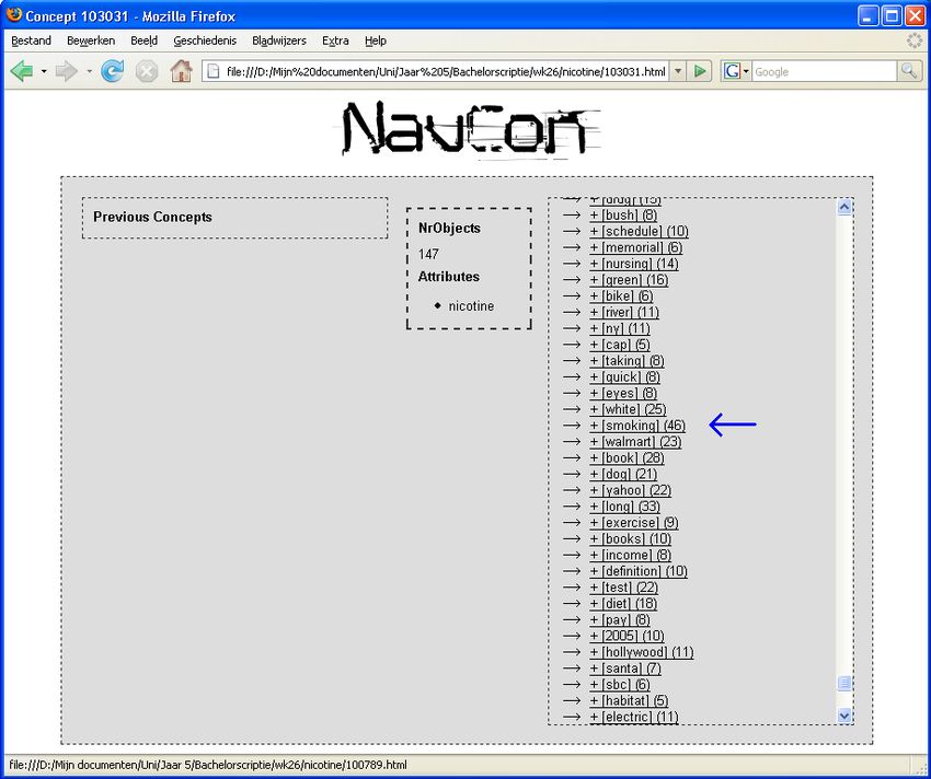
2
Contents

1   The AOL Scandal                                                                                                                                                    7
    1.1 Introduction . . . . . . . . . .              .   .   .   .   .   .   .   .   .   .   .   .   .   .   .   .   .   .   .   .   .   .   .   .   .   .   .   .    7
    1.2 Research on the AOL Scandal                   .   .   .   .   .   .   .   .   .   .   .   .   .   .   .   .   .   .   .   .   .   .   .   .   .   .   .   .    8
        1.2.1 Research Question . .                   .   .   .   .   .   .   .   .   .   .   .   .   .   .   .   .   .   .   .   .   .   .   .   .   .   .   .   .    8
        1.2.2 Sub Questions . . . . .                 .   .   .   .   .   .   .   .   .   .   .   .   .   .   .   .   .   .   .   .   .   .   .   .   .   .   .   .    9
    1.3 Outline of the Thesis . . . . .               .   .   .   .   .   .   .   .   .   .   .   .   .   .   .   .   .   .   .   .   .   .   .   .   .   .   .   .   10
        1.3.1 Parts . . . . . . . . . .               .   .   .   .   .   .   .   .   .   .   .   .   .   .   .   .   .   .   .   .   .   .   .   .   .   .   .   .   10
        1.3.2 Chapters . . . . . . . .                .   .   .   .   .   .   .   .   .   .   .   .   .   .   .   .   .   .   .   .   .   .   .   .   .   .   .   .   10

2   Search Engines                                                                                                                                                    13
    2.1 Introduction . . . . .    .   .   .   .   .   .   .   .   .   .   .   .   .   .   .   .   .   .   .   .   .   .   .   .   .   .   .   .   .   .   .   .   .   13
    2.2 History Of Searching      .   .   .   .   .   .   .   .   .   .   .   .   .   .   .   .   .   .   .   .   .   .   .   .   .   .   .   .   .   .   .   .   .   13
    2.3 Why they work . . .       .   .   .   .   .   .   .   .   .   .   .   .   .   .   .   .   .   .   .   .   .   .   .   .   .   .   .   .   .   .   .   .   .   13
    2.4 The Structure . . . .     .   .   .   .   .   .   .   .   .   .   .   .   .   .   .   .   .   .   .   .   .   .   .   .   .   .   .   .   .   .   .   .   .   14
    2.5 Web Crawling . . . .      .   .   .   .   .   .   .   .   .   .   .   .   .   .   .   .   .   .   .   .   .   .   .   .   .   .   .   .   .   .   .   .   .   14
    2.6 Indexing . . . . . . .    .   .   .   .   .   .   .   .   .   .   .   .   .   .   .   .   .   .   .   .   .   .   .   .   .   .   .   .   .   .   .   .   .   15
    2.7 Searching . . . . . . .   .   .   .   .   .   .   .   .   .   .   .   .   .   .   .   .   .   .   .   .   .   .   .   .   .   .   .   .   .   .   .   .   .   16
         2.7.1 Tf-idf . . . . .   .   .   .   .   .   .   .   .   .   .   .   .   .   .   .   .   .   .   .   .   .   .   .   .   .   .   .   .   .   .   .   .   .   16
         2.7.2 PageRank . .       .   .   .   .   .   .   .   .   .   .   .   .   .   .   .   .   .   .   .   .   .   .   .   .   .   .   .   .   .   .   .   .   .   17
    2.8 The AOL Search Data       .   .   .   .   .   .   .   .   .   .   .   .   .   .   .   .   .   .   .   .   .   .   .   .   .   .   .   .   .   .   .   .   .   18

3   Laws in Computational Linguistics                                                                                                                                 19
    3.1 Introduction . . . . . . . . . . .                .   .   .   .   .   .   .   .   .   .   .   .   .   .   .   .   .   .   .   .   .   .   .   .   .   .   .   19
    3.2 Zipf’s Law . . . . . . . . . . . .                .   .   .   .   .   .   .   .   .   .   .   .   .   .   .   .   .   .   .   .   .   .   .   .   .   .   .   19
        3.2.1 Mathematical . . . . . .                    .   .   .   .   .   .   .   .   .   .   .   .   .   .   .   .   .   .   .   .   .   .   .   .   .   .   .   20
    3.3 Heaps’ Law . . . . . . . . . . .                  .   .   .   .   .   .   .   .   .   .   .   .   .   .   .   .   .   .   .   .   .   .   .   .   .   .   .   20
        3.3.1 Mathematical . . . . . .                    .   .   .   .   .   .   .   .   .   .   .   .   .   .   .   .   .   .   .   .   .   .   .   .   .   .   .   21
    3.4 Link with the AOL Scandal . .                     .   .   .   .   .   .   .   .   .   .   .   .   .   .   .   .   .   .   .   .   .   .   .   .   .   .   .   21
        3.4.1 Stop Words . . . . . . .                    .   .   .   .   .   .   .   .   .   .   .   .   .   .   .   .   .   .   .   .   .   .   .   .   .   .   .   21

4   Formal Concept Analysis                                                                                                                                           23
    4.1 Introduction . . . . .    .   .   .   .   .   .   .   .   .   .   .   .   .   .   .   .   .   .   .   .   .   .   .   .   .   .   .   .   .   .   .   .   .   23
    4.2 Concepts . . . . . . .    .   .   .   .   .   .   .   .   .   .   .   .   .   .   .   .   .   .   .   .   .   .   .   .   .   .   .   .   .   .   .   .   .   23
    4.3 Formal Concepts . .       .   .   .   .   .   .   .   .   .   .   .   .   .   .   .   .   .   .   .   .   .   .   .   .   .   .   .   .   .   .   .   .   .   24
    4.4 Formal Definition . .     .   .   .   .   .   .   .   .   .   .   .   .   .   .   .   .   .   .   .   .   .   .   .   .   .   .   .   .   .   .   .   .   .   24
    4.5 Concept Lattices . . .    .   .   .   .   .   .   .   .   .   .   .   .   .   .   .   .   .   .   .   .   .   .   .   .   .   .   .   .   .   .   .   .   .   25

                                                                  3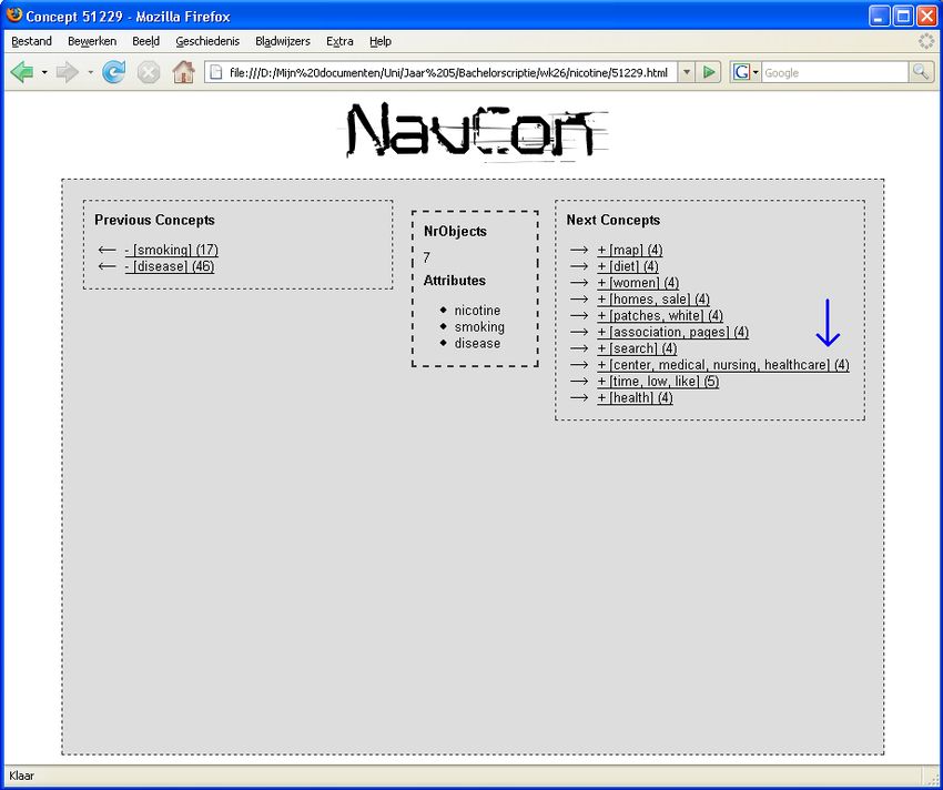
4 CONTENTS
4.6 Finding Formal Concepts . . . . . . . . . . . . . . . . . . . . . . . . . . . . . . 26
4.6.1 Basic . . . . . . . . . . . . . . . . . . . . . . . . . . . . . . . . . . . . . . 26
4.6.2 Meet and Join . . . . . . . . . . . . . . . . . . . . . . . . . . . . . . . . . 27
4.6.3 Ganter . . . . . . . . . . . . . . . . . . . . . . . . . . . . . . . . . . . . . 27
5 Meta Experiments 29
5.1 Introduction . . . . . . . . . . . . . . . . . . . . . . . . . . . . . . . . . . . . . . 29
5.2 General Statistics . . . . . . . . . . . . . . . . . . . . . . . . . . . . . . . . . . . 29
5.3 Checking . . . . . . . . . . . . . . . . . . . . . . . . . . . . . . . . . . . . . . . . 30
5.3.1 Lines of Data . . . . . . . . . . . . . . . . . . . . . . . . . . . . . . . . . 30
5.3.2 Instances of New Queries . . . . . . . . . . . . . . . . . . . . . . . . . . 30
5.3.3 Next Page Requests . . . . . . . . . . . . . . . . . . . . . . . . . . . . . 31
5.3.4 Click-through Events . . . . . . . . . . . . . . . . . . . . . . . . . . . . . 31
5.3.5 Queries without Click-through . . . . . . . . . . . . . . . . . . . . . . . 31
5.3.6 Unique Queries . . . . . . . . . . . . . . . . . . . . . . . . . . . . . . . . 32
5.3.7 Unique ID’s . . . . . . . . . . . . . . . . . . . . . . . . . . . . . . . . . . 32
5.4 Queries per Day . . . . . . . . . . . . . . . . . . . . . . . . . . . . . . . . . . . . 33
5.4.1 Rythm . . . . . . . . . . . . . . . . . . . . . . . . . . . . . . . . . . . . . 33
5.4.2 Missing Day . . . . . . . . . . . . . . . . . . . . . . . . . . . . . . . . . . 33
5.5 Conclusion . . . . . . . . . . . . . . . . . . . . . . . . . . . . . . . . . . . . . . . 34
6 Linguistic Experiments 35
6.1 Introduction . . . . . . . . . . . . . . . . . . . . . . . . . . . . . . . . . . . . . . 35
6.2 Zipf and the AOL data . . . . . . . . . . . . . . . . . . . . . . . . . . . . . . . . 35
6.2.1 AOL Word Counter . . . . . . . . . . . . . . . . . . . . . . . . . . . . . 35
6.2.2 Test Results . . . . . . . . . . . . . . . . . . . . . . . . . . . . . . . . . . 36
6.2.3 Mathematical . . . . . . . . . . . . . . . . . . . . . . . . . . . . . . . . . 36
6.3 Heaps and the AOL data . . . . . . . . . . . . . . . . . . . . . . . . . . . . . . . 36
6.3.1 Modifying AOL Word Counter . . . . . . . . . . . . . . . . . . . . . . . 36
6.3.2 Test Results . . . . . . . . . . . . . . . . . . . . . . . . . . . . . . . . . . 37
6.3.3 Mathematical . . . . . . . . . . . . . . . . . . . . . . . . . . . . . . . . . 38
6.4 Stop Words . . . . . . . . . . . . . . . . . . . . . . . . . . . . . . . . . . . . . . . 38
7 Conceptual Experiments 39
7.1 Introduction . . . . . . . . . . . . . . . . . . . . . . . . . . . . . . . . . . . . . . 39
7.2 Searching for Formal Concepts . . . . . . . . . . . . . . . . . . . . . . . . . . . 39
7.3 AOL Reader . . . . . . . . . . . . . . . . . . . . . . . . . . . . . . . . . . . . . . 39
7.4 Limiting to Sub Lattice . . . . . . . . . . . . . . . . . . . . . . . . . . . . . . . . 40
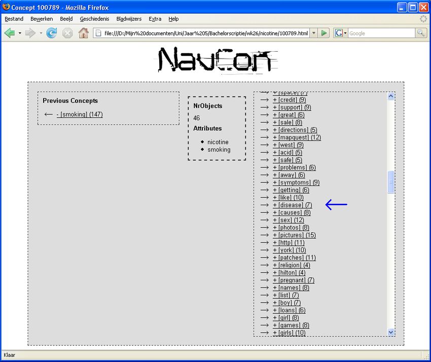
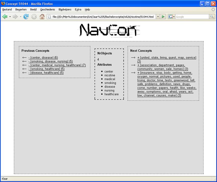
7.5 NavCon . . . . . . . . . . . . . . . . . . . . . . . . . . . . . . . . . . . . . . . . 41
7.5.1 Reading Concepts . . . . . . . . . . . . . . . . . . . . . . . . . . . . . . 42
7.5.2 Reduction Engine . . . . . . . . . . . . . . . . . . . . . . . . . . . . . . . 42
7.5.3 Writing the Output . . . . . . . . . . . . . . . . . . . . . . . . . . . . . . 43
7.6 Conclusion . . . . . . . . . . . . . . . . . . . . . . . . . . . . . . . . . . . . . . . 45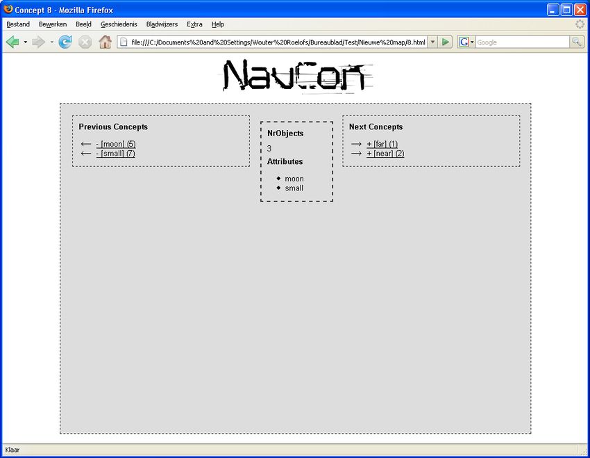
CONTENTS                                                                                                                                            5

8   Conclusions                                                                                                                                    49
    8.1 Conclusion 1 . . . . . . . . . . . . . .   .   .   .   .   .   .   .   .   .   .   .   .   .   .   .   .   .   .   .   .   .   .   .   .   49
    8.2 Conclusion 2 . . . . . . . . . . . . . .   .   .   .   .   .   .   .   .   .   .   .   .   .   .   .   .   .   .   .   .   .   .   .   .   49
    8.3 Conclusion 3 . . . . . . . . . . . . . .   .   .   .   .   .   .   .   .   .   .   .   .   .   .   .   .   .   .   .   .   .   .   .   .   50
    8.4 Main Conclusion . . . . . . . . . . .      .   .   .   .   .   .   .   .   .   .   .   .   .   .   .   .   .   .   .   .   .   .   .   .   50
    8.5 Future Research . . . . . . . . . . . .    .   .   .   .   .   .   .   .   .   .   .   .   .   .   .   .   .   .   .   .   .   .   .   .   50
        8.5.1 Applying Heuristics . . . . .        .   .   .   .   .   .   .   .   .   .   .   .   .   .   .   .   .   .   .   .   .   .   .   .   51
        8.5.2 Practical Solutions . . . . . .      .   .   .   .   .   .   .   .   .   .   .   .   .   .   .   .   .   .   .   .   .   .   .   .   51
        8.5.3 Availability & Computability         .   .   .   .   .   .   .   .   .   .   .   .   .   .   .   .   .   .   .   .   .   .   .   .   52

A The AOL Search Data in SQL                                                                                                                       53
6 CONTENTS
Chapter 1

The AOL Scandal

1.1      Introduction
Today, the World Wide Web is more important than ever. Practically everyone (in West-
ern countries) uses the internet daily as a main source of information and communication.
Google, the worlds largest search engine, is known and used all over the world and tries
to ‘organize the world’s information and make it universally accessible and useful’. Given
these facts, it is not hard to imagine that many people all over the world work in the branch
of Information Retrieval.
     Both the academic and the business world spend a lot of effort in this field. Researchers
everywhere try to contribute to Information Retrieval by thinking up new and better ways
of finding information and businesses everywhere try to implement these ideas and make a
living out of it. The same goes for America OnLine (AOL), a global web services company
that provides services for millions of people worldwide. It provides internet connections,
instant messaging, e-mail service and their large social network to its customers. In some of
those fields, like instant messaging, they are the largest in the U.S.
     One of the major problems for the researchers on Information Retrieval is the lack of real
life data. Search engines like Google keep this information secret for obvious reasons. This
does give the academic world a headache since they can improve their research if they had
this data. And going to work for Google is not an option for most of them. Three employees
of AOL, however, knew the scientific community hardly had any live data. Therefore, they
announced they would release 3 months of search data from AOL’s customers on The First
International Conference on Scalable Information Systems in Hong Kong in June 2006 [2].
Unfortunately for them, it did not work out to their advantage. Their action set the following
events in motion:

August 4, 2006 AOL released a compressed text file on one of its websites containing twenty
    million search keywords for over 650,000 users over a 3-month period, intended for
    research purposes.

August 7, 2006 AOL pulled the file from public access, but not before it had been mirrored,
    P2P-shared and seeded via BitTorrent. News filtered down to the blogosphere1 and
    popular tech sites such as Digg and Wired News.
  1
      Blogosphere is the collective term encompassing all blogs as a community or social network

                                                       7
8 CHAPTER 1. THE AOL SCANDAL
August 7-21, 2006 The following weeks the media continued exploring this hot issue, now
named the AOL Scandal. The New York Times for example, tried to identify indi-
viduals by looking for names, addresses, social security numbers, etcetera in the data.
They managed to track down several persons by cross referencing this data with phone
books or other public records. A hefty ethics debate was the result.
August 21, 2006 AOL took the matter quite seriously which led to the resignation of AOL’s
CTO, Maureen Govern, the researcher who released the data, and his immediate su-
pervisor, who reported to Govern.
September 7, 2006 I get my hands on a copy of the AOL search data, looked into the story
behind it and decided to start this research.
September 22, 2006 A class action lawsuit is filed against AOL in the U.S. District Court for
the Northern District of California. ”The lawsuit accuses AOL of violating the Elec-
tronic Communications Privacy Act and of fraudulent and deceptive business prac-
tices, among other claims, and seeks at least $5,000 for every person whose search data
was exposed”, says Elinor Mills in her news blog. This adds up to a possible total
amount of $3,250,000,000.
1.2 Research on the AOL Scandal
The growth of the internet and the way practically everyone uses it nowadays comes with
a downside; our personal information can become freely available to everyone on the web.
Therefore the discussion of privacy and especially digital privacy has become a pressing
issue. Reason enough to have a look at this so-called AOL Scandal.
This AOL search data was released with the intention of stimulating academic researchers,
so there must be something of value in it. There are many possible researches to be done
with it. For example, it can be used to provide (relevant) feedback to the technique on find-
ing useful search results. Or it can give information on who searchers judge the relevance
of certain (types of) pages when searching on a certain query. Research can also be done on
the composition of the average query in respect to what the searcher was actually looking
for. Advertising companies might be interested in searching behaviour to address people
personally.
After considering some of these options, the focus for this research was formulated.
Keeping with my interest in Information Retrieval and specifically in Formal Concept Anal-
ysis (FCA), I decided to look at how the methods of FCA could be applied to (parts of) the
AOL search data with the idea of uncovering some implicit links between people and their
searching behaviour. Combining this with the hot issues of privacy and this so called AOL
Scandal, I decided this was a feasible research for a bachelor thesis in Information Sciences.
1.2.1 Research Question
As with all good research, a research question was formulated for this research and divided
into smaller questions which can (hopefully) be answered to answer the main question. The
research question is as follows:1.2. RESEARCH ON THE AOL SCANDAL 9
Is it possible to classify groups of people by their searching behaviour in an automated
way using Formal Concept Analysis?
This question is quite specific and narrowed down, because a more general question
would be too vague, leading to an unresearchable whole. The focus on classification is jus-
tifiable, because this fits quite nicely with the knowledge on and possible outcomes of FCA.
On top of that, the possible affirmative outcome could be interpreted as an indication that
further research on this subject could be wise. The results could also have a pragmatic value,
which will be discussed in the final chapter of this thesis.
1.2.2 Sub Questions
In order to answer the main research question and to address some interesting side-issues,
the following sub questions have been formulated, each with an explanation:
1. Is the integrity of the data good enough to support valid outcomes?
One of the main ideas behind this research is that FCA can be applied to the AOL
search data with a meaningful outcome because the data is fully representative for
other real live search data. If the data set used for the research turns out to be com-
promised or manually adjusted, the whole outcome can be flawed and questioned.
Therefore some meta-research must be done on the data as a whole.
2. Is there an indication that the data supports FCA?
The research data may be one of the few real live sets on which FCA research get
done, but it certainly is not the first. Previous research on the subject of Information
Retrieval and more specifically FCA lead to some interesting results [6] that might
also apply to this research. Therefore some statistical analysis will be done that will
hopefully indicate that the data show some of the same features as other data sets used
for FCA research.
3. Does applying FCA to the data lead to relevant results?
As a third step in the process the actual FCA will be executed. The results of these
experiments play the most important role in answering the main research question.
Two small side notes to reading the rest of this thesis:
1. The terms ‘the data’, ‘the search data’, ‘the research data’ and ‘the AOL data’ will all
be used next to each other to denote the same thing, the AOL search data.
2. This thesis will obviously not contain any data that can actually be tracked back to
individuals as this would be inappropriate and more importantly not ‘done’.
In order to answer these questions several methods will be used. Existing literature will be
consulted on Information Retrieval techniques. Internet sources like renown news portals
provide necessary information on the AOL Scandal itself. The practical part of the research
will be done in a demo setting, using a copy of the AOL search data to do several experiments
on. Because of the specific nature of the data, tools probably need to be made to exercise
these experiments. Finally, there will be a presentation of the research done.10 CHAPTER 1. THE AOL SCANDAL
1.3 Outline of the Thesis
The thesis before you is the bachelor thesis of Wouter Roelofs, an Information Science stu-
dent at the Radboud University of Nijmegen. The thesis is supervised by Dr. Franc Grootjen,
who is specialized in the field of Information Retrieval. The thesis’ structure is described in
the rest of this section.
1.3.1 Parts
The thesis roughly consists out of five parts. The first is an introductory part that introduces
the problem and describes the research plan. The second part will be a theoretical part, de-
scribing background information that support (the understanding of) the experiments. The
third part contains the experiments themselves. This part has close links with the theoretical
part. Their chapters can be mapped almost 1:1. The fourth part is the end of the research,
which answers the question from the first. The fifth is an appendix part, this provides some
additional information for completeness.
1.3.2 Chapters
Part 1 consists of just one chapter, the current one. It started with the introduction of the so-
called AOL Scandal, giving a basic overview of events and the media circus around it. This
is followed by the research plan, detailing what exactly will be researched. And it contains
an outline of the thesis.
Part 2 has three chapters. Chapter 2 explains what search engines are and how they work.
Some laws on computational linguistics are described in chapter 3. Chapter 4 provides you
with an elaborate explanation of a data mining method called Formal Concept Analysis.
This concludes the second part.
Part 3 is the practical part and also has three chapters. Chapter 5 covers some meta
experiments on the data to ensure its usefulness. Chapter 6 links back to chapter 3 and
tries to apply the linguistic laws to the research data. Chapter 7 then brings the theory from
chapter 4 in practise in the experiments that will hopefully answer the main question.
The final real part of the thesis, part 4 will again have just one chapter. Chapter 8 is a typ-
ical conclusions chapter, answering the research questions. It also contains some thoughts
on what continuing research could be done in the future.
For completeness, appendix A describes the way the research data was transformed into
a more processable form.
Figure 1.1 sums up the structure of the thesis. To get a quick impression of the research,
read the introduction and the conclusion chapters, chapters 1 and 8. Readers that are already
familiar with the theory behind search engines, computational linguistics and FCA can skip
the theoretical part and continue reading in chapter 5. People interested in the whole thing,
simply continue in chapter 2.1.3. OUTLINE OF THE THESIS 11
Chapter 1
Introduction
Theoretical
Chapter 2
Search Engines
Chapter 3
Comp. Laws
Chapter 4
FCA
Practical
Chapter 5
Meta Exp.
Chapter 6
Linguistic Exp.
Chapter 7
Conceptual Exp.
Chapter 8
Conclusions
Figure 1.1: Outline of the Thesis12 CHAPTER 1. THE AOL SCANDAL
Chapter 2

Search Engines

2.1     Introduction
The search engine used by America OnLine is not actually their own search engine, it is a
portal to Google. Buying existing search technique is a smart thing to do when you are not
in that line of business yourself. And Google is the worlds largest search engine after all.
    So the research data, the AOL search data, is actually mostly Google’s data; just the
notion of which person is searching is what AOL keeps track of. This is because those per-
sons are logged in using their AOL account. The rest of the searching process gets done by
Google. Of course we need to know what exactly we are looking at. Therefore this chapter
will provide background information on how search engines work.

2.2     History Of Searching
Searching for information is something human kind has done since the beginning. We are
always in a conquest for finding new information, because we believe knowledge can make
us stronger1 . In fact, computers were made to do information searching. Searching is a very
structured but time consuming task, therefore we made a machine that could do it for us.
    With the coming of the internet, the accessibility to information has been multiplied by a
large factor. But with more information comes more trouble finding exactly what you want.
And so the need for an internet search engine was born. The very first tool for searching the
internet dates back to 1990, but this was a quite primitive system only capable of searching
in filenames. The first real web search engine, called Wandex, was developed in 1993 and
could search inside documents. The well-known search engine Google started in 2000 and
added a couple of smart features to enhance the search results. Nevertheless, Google still
operates in more or less the same way as any other search engine.

2.3     Why they work
When designing an automatized search engine you immediately encounter a problem: A
computer cannot think like humans, a computer cannot reason, it can simply follow orders.
   1
    The author is aware of the fact that information is not equivalent to knowledge, but this is a whole other
discussion which lies outside the scope of this research

                                                     13
14 CHAPTER 2. SEARCH ENGINES
And people do not always know exactly what they are looking for either. After all, if you
knew exactly what document you were looking for, you would not have to look for it! That
is why you need to think up a way to communicate with the computer to ‘explain’ what it is
you are looking for. And on the other side, the computer needs some sort of representation
of the knowledge at hand and a way to match both.
This is why almost all automated retrieval systems use a variant of the term-based dis-
closure system. The main principle in this approach is that terms hold a descriptive (con-
ceptual) value. These systems try to characterise documents using word sets. The words
are normally taken from the document in an automated fashion. Essentially these systems
assume that:
If a certain word occurs in a document, that document is about that word.
Note that word order plays no role in these models. Consider the famous example of a docu-
ment called ‘The Hillary Clinton Bill Proposal’ which contains the words ‘Bill’ and ‘Clinton’.
It illustrates the importance of word order, which is lost in this approach. Matching in this
model involves comparing word occurrences in query and characterisations, which can be
done in numerous ways. All term-based models rely on the following hypothesis:
If a document and the query have a word in common, the document is likely to be relevant.
And the funny thing about this is that this seems to work. Up to today, most efforts done
by linguistic researchers on using word syntactics or semantics to improve search systems
have resulted in systems that are not much better than these simple systems of counting
which words occur in a certain document and which do not.
2.4 The Structure
A typical web search engine consists of three parts: Web Crawling, Indexing and Searching.
The internet is a worldwide network between computers, therefore no-one has all the data
on the web stored internally. This makes it a bit harder to ‘know’ what information you
have got. If you compare it to having a number of files on your computer. If you would
like to search in them, you can always simply access them, you know if they were changed,
etcetera. The internet is not like that, therefore there is the technique called Web Crawling,
this part handles the locating of web pages. When you found those web pages, you would
probably like to know what is inside them, so you can give a more accurate search result
to the searcher. This is done by the second part, the Indexing. And finally there is the part
where a person actually sits behind its desk and would like to find a web page containing
the information he was hoping for, Searching.
2.5 Web Crawling
Staying with the metaphor of the internet being a web of computers, web crawlers are often
called spiders. They are little programs that ‘walk’ the web looking for web pages and doing
some additional work on the way, such as keeping statistics. But how do you find (almost)
every page on the web? Web crawlers do this by simply following the links on each page
to a next page. These links were made by the designers of the web pages and together they2.6. INDEXING 15
make a complete web of pages. Logically search engines like Google also offer people that
just made a new website the opportunity to tell them where it is. This gives web crawlers a
new page to start crawling.
There are two different styles of crawling, depth-first and breadth-first. In the first case
when a spider comes across a link, it immediately follows it and goes back following other
links when it reaches a dead end. If you would draw a schematic picture of this situation,
putting the first page at the top and every page it links to beneath it, you will see that by this
way of walking through the pages the spider goes deep first, hence the name depth-first.
In the second case, the spider queues up all the links on a page and then follows them in
that order before moving to the next level of deepness. This time the spider goes wide first,
then goes deep. See figure 2.1 for an example. The breadth-first is the more popular choice
because it results in higher quality pages.
Figure 2.1: Depth-first versus Breadth-first
Please note that this is a simplified view on how a web crawler works. In practice
many techniques have been thought up over the years to enhance the work of web crawlers.
Among these techniques are: clever selecting of pages, avoiding getting into endless loops,
path-ascending crawling, focused crawling and revisiting. A more detailed overview of
crawlers and crawling techniques unfortunately lies beyond the scope of this research.
2.6 Indexing
When a spider reaches a web page, it needs to do something with it so that the search engine
know this page exists and what it is about. After all, we want to provide the searchers
with the best fitting answers. Therefore, we index. Obviously we will not save the pages
as a whole, because every search engine would then hold a copy of the internet on their
computers. That is why people needed to come up with a better idea on how to keep track
of the contents of a page.
As we saw before, the system we use is based on counting the occurrence of words and
that is exactly what is done when indexing. In the case of Google, the indexing is done by
the same piece of software that does the crawling, the spider. So it has crawled to a certain
web page and now it simply goes over the contents of the (source of) the page and tallies
the words and their occurrences. Modern indexing software does a bit more than simple
tallying work, but it still is the main idea behind and strength of web search engines.
A couple of important properties of indexing are: the size of the index, the speed of
looking things up, the way the indexed data is stored and maintenance of the index over16 CHAPTER 2. SEARCH ENGINES
time. For many of these issues clever solutions have been thought up, but those are not in
the scope of this research.
What still needs to be mentioned however is the way the index is kept, because this
affects the way you can search in it later on. Many search engines incorporate an inverted
index. This means that, instead of keeping a list of documents and per document their
words, it keeps a list of all words used and per word which document it occurs in. See
table 2.1 for an example.
Word Documents
the Document 1, Document 3, Document 4, Document 5
cow Document 1, Document 2, Document 3, Document 4
says Document 1, Document 5
moo Document 1, Document 7
Table 2.1: An inverted index
2.7 Searching
Finally we come to the actual searching. Now we have an inverted index of a set of doc-
uments on the internet and there is a certain information need from a searcher. We have
already seen that if a document and the query have a word in common, the document is
likely to be relevant. And we have seen that the technique most search engines use is a rela-
tively simple one, since it only deals with word occurrences in documents instead of actual
language semantics. It does not come as a surprise then that the search part of search engines
is term-based too.
The searcher formulates his information need in a so-called query which seems to be a
highly unstructured and ambiguous construct. For example, when I am searching for a web
page on magical squares, my query could simply be ‘magical squares’. Both words can mean
many things, when I say ‘magical’ you could think about magicians, illusionists or even
simply amazing things. ‘Squares’ could indicate a square in a city, like the famous Trafalgar
Square. Nevertheless a search engine will come up with exactly the web pages I would
like to see, about the mathematical phenomenon. So how does an automated system with
no actual knowledge do this. We will now look at two ways, using the ‘classical’ weight
tf-idf and using the technique that contributed to making Google so incredibly popular:
PageRank.
2.7.1 Tf-idf
The tfidf weight (term frequencyinverse document frequency) is a weight often used in In-
formation Retrieval and text mining [11]. This weight is a statistical measure used to evaluate
how important a word is to a document in a collection or corpus. The importance increases
proportionally to the number of times a word appears in the document but is offset by the
frequency of the word in the corpus.
The term frequency in the given document is simply the number of times a given term
appears in that document. This count is usually normalized to prevent a bias toward longer2.7. SEARCHING 17
documents (which may have a higher term frequency regardless of the actual importance
of that term in the document) to give a measure of the importance of the term ti within the
particular document.
ni
tfi = P
k nk
where ni is the number of occurrences of the considered term, and the denominator is
the number of occurrences of all terms.
The inverse document frequency is a measure of the general importance of the term (ob-
tained by dividing the number of all documents by the number of documents containing the
term, and then taking the logarithm of that quotient).
|D|
idfi = log
|{d : d 3 ti }|
with
• |D| : total number of documents in the corpus
• |{d : d 3 ti }| : number of documents where the term ti appears (that is ni 6= 0).
Then
tfidf = tf · idf
A high weight in tfidf is reached by a high term frequency (in the given document) and
a low document frequency of the term in the whole collection of documents; the weights
hence tends to filter out common terms.
And so search engines calculate the tf-idf weight for a given query and displays the
documents that have the highest rating, ordered by that rating of course.
2.7.2 PageRank
Using the tf-idf weight works surprisingly well, high results have been made by it, especially
after improving it with some smart tricks. If you are searching for a web page on magical
squares however and a certain web page is a phony web simply containing the words ‘magi-
cal’ and ‘squares’ a lot of times, it would result in a high tf-idf score, thus would be assumed
to be very fitting to your request. But you probably do not want this page, therefore Larry
Page, Co-Founder & President of Products of Google Inc, developed PageRank.
PageRank is a link analysis algorithm that assigns a numerical weighting to each element
of a hyperlinked set of documents, such as the World Wide Web, with the purpose of ”mea-
suring” its relative importance within the set. A simple description of PageRank by Google:
‘PageRank relies on the uniquely democratic nature of the web by using its vast link struc-
ture as an indicator of an individual page’s value. In essence, Google interprets a link from
page A to page B as a vote, by page A, for page B. But, Google looks at more than the sheer
volume of votes, or links a page receives; it also analyzes the page that casts the vote. Votes
cast by pages that are themselves ”important” weigh more heavily and help to make other
pages ”important”’.
PageRank is a probability distribution used to represent the likelihood that a person ran-
domly clicking on links will arrive at any particular page. PageRank can be calculated for18 CHAPTER 2. SEARCH ENGINES
any-size collection of documents. It is assumed in several research papers that the distri-
bution is evenly divided between all documents in the collection at the beginning of the
computational process. The PageRank computations require several passes, called ”itera-
tions”, through the collection to adjust approximate PageRank values to more closely reflect
the theoretical true value.
The (simplified) PageRank algorithm uses the following equation:
1−d X P R(pj )
P R(pi ) = +d
N L(pj )
pj ∈M (pi )
where p1 , p2 , ..., pN are the pages under consideration, M (pi ) is the set of pages that link
to pi , L(pj ) is the number of outbound links on page pj , and N is the total number of pages.
Using this PageRank algorithm Google is able to get even better fitting results for search
queries than the original tf-idf approach. Going into these techniques in more extend goes
beyond the scope of the research.
2.8 The AOL Search Data
The AOL search data is data of the third part, so it is data of the actual search process done
by humans. It contains queries by users and the results that the AOL search portal gave
(through Google). The really interesting part is that the queries are linked to users, although
anonymized. This is information you would normally not have, since you do not have to
login to use Google. Google could of course log your ip-address, but that would not give
much assurance as people might have a dynamic ip or go to school and search there. And
it could be that a lot of people search from the same ip-address. This makes the AOL search
data interesting to experiment with.
We conclude this chapter with the following figure that sums it up.
knowledge information need
gap N
request characterization
formulation q χ indexing
searcher matching collection
Figure 2.2: The Information Retrieval Paradigm
A searcher had a knowledge gap, which leads to an information need N . The searcher
formulates his information need in a request q. From the other side, there is a collection of
documents. By indexing the characterization χ of the documents. Finally, these two sides
come together in the processing of matching, so the searcher can find the documents that fill
his knowledge gap.Chapter 3
Laws in Computational Linguistics
3.1 Introduction
In order to fully understand the reason behind the experiments described in chapter 6 we
must first look at language and, more specifically, at some unwritten laws that appear in
language. The laws we are talking about are called Zipf’s law and Heaps’ law. Both Zipf and
Heaps found logical patterns in (natural) language and formulated these in mathematical
laws.
This chapter will present these laws, their characteristics and properties and will hope-
fully provide enough background information for chapter 6.
3.2 Zipf’s Law
There are many models that, given the probability of certain events, try to describe the prob-
ability of a sequence of those events. The most well-known models that try to connect these
probabilities are Zipf’s Law [16] and the Mandelbrot distribution [10].
Zipf’s Law states that, in many practical situations, if the r-th most probable event has
probability p, then p · r is (almost) equal for all events. The Mandelbrot distribution claims
this for the expression p·(c+r)θ for some parameters c and θ. In case of c = 0, the distribution
is also referred to as the generalized Zipf’s Law. Some authors motivate the validity of these
laws from physical phenomena, see for example [15] for Zipf’s Law in the context of cities.
But it is also possible to derive Zipf’s law from a simple statistical model [9].
Probably the best known application of Zipf’s law is from linguistics: Zipf’s Law can
used to describe word frequencies in natural language input. For example Tolkien’s The Lord
of The Rings [12] produces figure 3.1 when we plot word frequencies against word ranks on
a double log scale.
The simplest case of Zipf’s law is a ”1/f function”. Given a set of Zipfian distributed fre-
quencies, sorted from most common to least common, the second most common frequency
will occur 1/2 as often as the first. The third most common frequency will occur 1/3 as often
as the first. The nth most common frequency will occur 1/n as often as the first. And this
is exactly what we see in figure 3.1. However, this cannot hold precisely true, because items
must occur an integer number of times: there cannot be 2.5 occurrences of a word. This is
the reason why we stated ‘is (almost) equal’ before. Nevertheless, over fairly wide ranges,
and to a fairly good approximation, many natural phenomena obey Zipf’s Law.
1920 CHAPTER 3. LAWS IN COMPUTATIONAL LINGUISTICS
100000
lotr
Zipf’s Law
10000
frequency
1000
100
10
1 10 100 1000
rank
Figure 3.1: Word frequencies from The Lord of the Rings
3.2.1 Mathematical
For completeness sake we conclude this section by showing the mathematical formulation
of Zipf’s Law. It can be formulated as:
1/k s
f (k; s, N ) = PN
s
n=1 1/n
where N is the number of elements, k is their rank, and s is the exponent characterizing the
distribution. In the example of the frequency of words in the English language, N is the
number of words in the English language and, if we use the classic version of Zipf’s law, the
exponent s is 1.
3.3 Heaps’ Law
Another (experimental) law of nature is Heaps’ Law [7], which describes the growth in the
number of unique elements (also referred as the number of records), when elements are
drawn from some distribution.
Heaps’ Law states that this number will grow according to αxβ for some application
dependent constants α and β, where 0 < β < 1. In the case of word occurrences in natural
language, Heaps’ Law predicts the vocabulary size from the size of a text. In figure 3.2
this relationship is presented for The Lord of the Rings together with a fit1 of Heaps’ law for
α = 36.7 and β = 0.46.
A lot of (linguistic) research has been done to statistically describe word distributions.
Only the fact that languages are closed (having a finite number of words) or open has been
the source of a lot of discussion. In [8] a good historic overview is given. Furthermore it
contains an argumented claim that languages are open.
1
Fit has asymptotic standard error of 0.75% for α and 0.13% for β3.4. LINK WITH THE AOL SCANDAL 21
18000
lotr
16000 Heaps’ Law
14000
unique words 12000
10000
8000
6000
4000
2000
0
0 100000 200000 300000 400000 500000
word
Figure 3.2: Vocabulary growth of The Lord of the Rings
3.3.1 Mathematical
Like with Zipf’s Law, we shall quickly go over the mathematical definition of Heaps’ Law.
It can be formulated as:
VR (n) = αnβ
where VR is the subset of the vocabulary V represented by the instance text of size n. α
and β are free parameters determined empirically. With English text corpora, typically α is
between 10 and 100, and β is between 0.4 and 0.6. As we saw previously, this is the case
when looking at The Lord of the Rings.
3.4 Link with the AOL Scandal
What we have not discussed in this chapter yet is what these laws of language have to do
with the AOL Scandal. Our main assumption in this research was: The words a person looks
for tell us something about that person. So if the AOL Search Data would unconsciously
follow the same patterns as natural language, then these two laws might apply to them too.
This leaves us the opportunity to use some of the knowledge we have on natural language
and use it to our advantage on the research, like that of stop words.
3.4.1 Stop Words
Stop words are words that are generally seen as ‘less meaningful words’. The term was intro-
duced by Hans Peter Luhn, one of the pioneers in information retrieval, who used the con-
cept in his design and implementation of KWIC indexing programs. Typically, stop words
are adverbs and articles. Some examples are ‘the’, ‘a’, ‘in’, ‘of’. They are said to add less
information to linguistic constructions than for instance nouns. Nevertheless they have a
purpose. The purpose of stop words is twofold:22 CHAPTER 3. LAWS IN COMPUTATIONAL LINGUISTICS
1. Redundancy
Stop words have a redundancy function. Especially in spoken language where people
might not hear each other very well, stop words limit the amount of possible errors.
For example, when person A says to person B ‘it is in the pocket of my coat’, the words
‘in’ and ‘of’ makes it illogical for B to think A said ‘it is in the pocket of my boat’, since
boats do not have pockets. Therefore these little added words can add a lot to the
understanding. Note that this does not apply to written language.
2. Construction
Stop words also have a purpose in constructions: ‘in the closet’ means something com-
pletely different than ‘on the closet’. And ‘president’ means something different than
‘the president’. These stop words really add extra information in these cases. However,
if you would disregard constructions, their added meaning would decrease again.
This research uses a word model in which all words are used separately. In such a case,
words like ‘of’ and ‘in’ are treated equally to nouns. This could mean that leaving in stop
words is a somewhat bad idea. We will come back to this issue in chapter 6.Chapter 4
Formal Concept Analysis
4.1 Introduction
In previous chapters we have looked at some theoretical basics of subjects from the Infor-
mation Retrieval world. Chapter 2 has shown how search engines work and chapter 3
dealt with laws in computational linguistics. This final theoretical chapter will give a basic
overview of Formal Concept Analysis. After this chapter we will have enough knowledge
to conduct our experiments in hope of answering the research question.
Formal Concept Analysis, from here on abbreviated to FCA, is a method of data analy-
sis that was introduced in 1982 by R. Wille [14] and applied in many quite different realms
like psychology, sociology, anthropology, medicine, biology, linguistics, computer sciences,
mathematics and industrial engineering. Worldwide there are dozens of academical insti-
tutes all doing research on the subject. But what is FCA and how can it be of use to us?
4.2 Concepts
FCA deals with concept. What exactly is a concept? According to Merriam-Webster a con-
cept is:
Main Entry: concept
Pronunciation: ’kn-"sept
Function: noun
Etymology: Latin conceptum, neuter of conceptus, past participle
of concipere to conceive -- more at CONCEIVE
1 : something conceived in the mind : THOUGHT, NOTION
2 : an abstract or generic idea generalized from particular
instances
This is a rather vague description, but it does give us an idea of what a concept is.
Merriam-Webster talks about ‘conceived in the mind’ so it has to do with human think-
ing. The description also says ‘abstract or generic idea’ so it has to do with abstracting from
specific examples and finding a higher level structure.
We will try to understand what a concept is with the following example. When you read
the word ‘chair’ somewhere, you probably know what is meant by it. Undoubtedly, you
have seen chairs because everyone uses them in daily life. Perhaps your neighbours have
2324 CHAPTER 4. FORMAL CONCEPT ANALYSIS
other chairs than you, but still you recognize them as being chairs. We can also explain what
a chair is by looking at what makes them chairs, their properties. You could say that a chair is
something with four legs, a back and is something to sit on. These are both ways of looking
at the concept chair.
4.3 Formal Concepts
It is only a short step from concepts to formal concepts; they have a lot in common. Never-
theless, a formal concept is, as the name predicts, formally defined thus (hopefully) easier to
grasp. To see what a formal concept is we will look at a returning example. It is an example
of the planets in our solar system. In our solar system, or context to keep it abstract, there
are nine planets: Mars, Neptune, Uranus, Saturn, Jupiter, Earth, Pluto, Venus and Mercury.
Some of these planets have moons circling around them, others do not. They all have a dis-
tance to the sun, some are nearer than others. And the planets differ in size too, some are
big, others small. We abbreviate these properties and put the planets and these properties in
a table, figure 4.1.
no moon
medium
moon
small
Planets
large
near
far
mars × × ×
neptune × × ×
uranus × × ×
saturn × × ×
jupiter × × ×
earth × × ×
pluto × × ×
venus × × ×
mercury × × ×
Figure 4.1: The planets context
In this context the planets Mars and Earth share the properties moon, near and small.
They are the only ones that share exactly these properties and they share no more properties.
The combination of these planets and these properties is therefore called a formal concept.
Formal concepts can prove to be quite intuitive too. The formal concept we just found can
be interpreted as ‘earth-like planets’, planets that can possibly harbor life.
4.4 Formal Definition
Now to make things really formal. We denote the collection of objects as O, the individual
members of this collection we write o1 , o2 etc, while we write subsets as O1 , O2 etc. The
same goes for the collection of attributes, but with A, a1 and A1 . In this definition we use
the words ‘objects’ and ‘attributes’, because it fits our planet example. You can abstract from4.5. CONCEPT LATTICES 25
these specific terms and talk about any given collections in which the members have a binary
relation to each other. The binary relation is defined as ∼⊆ O × A and:
o ∼ A ⇐⇒ ∀ o ∼ a
a∈A
a ∼ O ⇐⇒ ∀ a ∼ o
o∈O
For the relation ∼ we define the right polar function rightPolar: P(O) → P(A) as follows:
rightPolar(O) = {a ∈ A|a ∼ O}
And we define the left polar function leftPolar: P(A) → P(O) as:
leftPolar(A) = {o ∈ O|o ∼ A}
The rightPolar and leftPolar functions are in general not each others inverse. When they
are, a special situation occurs: a formal concept is a pair (O, A) ∈ P(O) × P(A) with:
rightPolar(O) = A
leftPolar(A) = O
rightPolar
Objects Attributes
leftPolar
Figure 4.2: The dualistic view with right and left polar function
4.5 Concept Lattices
These concepts can be partially ordered by inclusion: if (Oi , Ai ) and (Oj , Aj ) are concepts, we
define a partial order ≤ by saying that (Oi , Ai ) ≤ (Oj , Aj ) whenever Oi ⊆ Oj . Equivalently,
(Oi , Ai ) ≤ (Oj , Aj ) whenever Aj ⊆ Ai . Every pair of concepts in this partial order has a
unique greatest lower bound (meet) and a unique smallest upper bound (join), so this partial
order satisfies the axioms defining a lattice. T
The greatest lower bound of (Oi , Ai ) and (Oj , Aj ) is the concept with objects Oi Oj ; it
has as its attributes the union of Ai , Aj , and any additional attributes held by all objects in26 CHAPTER 4. FORMAL CONCEPT ANALYSIS
T
Oi T Oj . The smallest upper bound of (Oi , Ai ) and (Oj , Aj ) is the concept with attributes
Ai Aj ; it has T as its objects the union of Oi , Oj , and any additional objects that have all
attributes in Ai Aj .
In case of our example, a lattice of all concepts would look like figure 4.3. Each concept
in the lattice is only shown with its attributes. This has two reasons:
1. Adding the objects would make the figure unreadable.
2. The way it is now, you can clearly see the ordering of the concepts over the different
levels. For instance, the concept ({mars, earth},{moon, near, small}) we saw earlier
is a ‘larger’ concept than ({mars, earth, venus, mercury},{small, near}) and ({mars,
earth, pluto},{moon, small}), because those only have two of the three attributes. And
of course the other way around ‘smaller’ concepts have more objects than their direct
larger ones.
!sb
a
{small,
! ! moon,
!
\ a
bnear,
a far,
no
! !moon,
\ ba
medium, large}
aa
! !
\ b b aaa
! !!
\ b
b aaa
\
s! s \s bs aas
! ! b
{small,
L {moon,
, \ {moon,
l {moon,
L {moon,
near,
L ,
,
small,
\
far, ll far,L far,
no moon}
L , near} \
small} medium}
l L large}
L , \
l L
L , \
lL
Ls, s
\
lLs
{small,
J {moon,
l
l {moon,
%
near}J
J
small} l %
%far}
l
J l %
J %
s ls%
l
J
{small}
Z
Z {moon}
,
,
Z ,
Z ,
Z ,
Z
Zs,
Z ,
{}
Figure 4.3: Planets concept lattice
4.6 Finding Formal Concepts
There are several ways of finding (formal) concepts in a given context. We will look at three
examples: the simple, intuitive way that has a very high complexity, a somewhat intuitive
way that requires a lot less work but still is quite energy consuming and finally a clever
method that can really minimize the time needed to compute the concepts.
4.6.1 Basic
The first algorithm is the simplest and most straightforward. Simply generate all possible
subsets O from O and A from A and check whether (O, A) is a concept. You can check4.6. FINDING FORMAL CONCEPTS 27
abcde
abcd abce abde acde bcde
abc abd acd bcd abe ace bce ade bde cde
ab ac bc ad bd cd ae be ce de
a b c d e
Ø
Figure 4.4: order for E = {a, b, c, d, e}
whether (O, A) is a concept by applying the rightPolar function to O and see if you get A
and the leftPolar function to A and see if you get O. This method obviously is very time
consuming. Assuming n objects in O and m attributes in A, it has a complexity of 2n+m . The
number of concepts that can be found is bounded by min(2n , 2m ) [4].
4.6.2 Meet and Join
In practice, the number of concepts will be far less. As a consequence, it will be profitable
to bound the complexity of the generation algorithm to the actual number of concepts. And
that is what this second method does, it uses the knowledge of lattices. We know the con-
cepts are ordered, so we can formally derive a higher level concept from lower level con-
cepts. Therefore, we can generate the entire lattice by starting with the base concepts and
calculating the closure with respect to the join-operator [4]. And this is what the second
method does. As you can imagine this method is a lot more efficient since it no longer
checks all possible subsets of the objects and attributes collections. However, it is still rather
complex to calculate larger concepts from smaller ones. And since the number of concepts
has a size of O(n3 ) (where n is the number of attributes) [6], this method, especially for large
collections, is still not very fast.
4.6.3 Ganter
The third and last algorithm we will discuss here is the algorithm developed by Bernhard
Ganter [3]. The Ganter algorithm solves the major problem there is with the first method.
The major flaw in brute-force calculation of all concepts is that it simply does way too much
unnecessary work. Just a fraction of all possible subsets of the object and attributes collec-
tions need to be evaluated. And Ganter found a way to limit the amount of work.
He discovered that if you order all possible subsets of objects in a certain way, the Ganter
algorithm effectively goes depth-first through a binary tree (figure 4.4).
He then mathematically proved that that if a node in the order tree is a concept then the
branch will not yield any more concepts, [3]. Because of this Ganter’s algorithm can stop28 CHAPTER 4. FORMAL CONCEPT ANALYSIS
searching for concepts in certain branches and is faster than a brute force implementation,
which needs to check each possible subset of objects.
In 2006 Mark Blokpoel [1] did research on a parallel implementation of the Ganter algo-
rithm in Java. His implementation offers a clean and simple way of doing FCA. It supports
multiple forms of inputting contexts and outputting the resulting concepts. It does not how-
ever keep any notion of relations between concepts. A short excerpt from the output of
Blokpoel’s program after running the planets example:
mars
earth
moon
near
smallChapter 5
Meta Experiments
5.1 Introduction
The first step in a research should be to check the research data used for consistency. If the
data proves to be tempered with, made up or simply out of balance, the whole research can
be questioned. Therefore some meta-research must be done on the data. In this chapter the
data will be examined, compared to the claims AOL itself makes about it and checked for
any anomalies
5.2 General Statistics
The AOL search data has been spread in a plain text format, zipped into an archive file. The
original data file as published by AOL could be found at their research site under ‘500kUser-
QueriesSampledOver3Months’. Obviously, this file has been removed from their site. If you
are looking for the data however, you might still be able to find it mirrored somewhere. Such
a copy is used for this research.
The archive file is called AOL-user-ct-collection.rar and is approximately 321.079
kB in size. Inside we find a directory named AOL-user-ct-collection in which are 11
plain text files: U500k README.txt and ten files named user-ct-test-collection-{01
to 10}.txt. The first file explains what the collection is and what data is in it. The follow-
ing statistical information is from that file:
Basic Collection Statistics
Dates:
01 March, 2006 - 31 May, 2006
Normalized queries:
36,389,567 lines of data
21,011,340 instances of new queries (w/ or w/o click-through)
7,887,022 requests for "next page" of results
19,442,629 user click-through events
16,946,938 queries w/o user click-through
10,154,742 unique (normalized) queries
657,426 unique user ID’s
2930 CHAPTER 5. META EXPERIMENTS
As you can see this is all statistical information on meta-level. statistical information on
the actual data will be discussed in chapter 6.
To make the data a bit easier to handle, it has been read into a MySQL database. Now the
power of querying the data can be exploited using the SQL syntax, which makes it easier to
gather or check simple information like how many queries are there. Basic knowledge about
SQL is recommended for further reading. If you are unfamiliar with SQL, you can check the
Wikipedia page on it. For detailed information on the database structure and the method
used to insert the AOL data into the database, see appendix A.
5.3 Checking
A first step is to check whether these general statistics as claimed by AOL are correct. Since
we have the SQL database and therefore the power of SQL, this can be done with ease.
5.3.1 Lines of Data
Checking the total number of lines is quite easy.
mysql> SELECT COUNT(*)
-> FROM data;
+----------+
| COUNT(*) |
+----------+
| 36389567 |
+----------+
1 row in set (0.08 sec)
AOL said there were 36,389,567 lines of data so this is correct.
5.3.2 Instances of New Queries
Instances of new queries is a bit trickier. The AOL read-me file describes the different situa-
tions you can have while searching on the internet and how these are stored in the AOL data.
One of the things it describes is how ‘next page of results’ are saved. Whenever a user did
a query, but did not find what he was looking for, he goes to the next page of results. This
appears in the search data as two different lines, containing the same query, but with a later
time stamp. As an opposite there are of course the queries that did not result in a next page
requests and as you can imagine, these two numbers should add up to the total number of
queries done. Let’s begin with looking at the new instances of queries, so the ones that are
not a next page request.
mysql> SELECT anonid, query, COUNT(*)
-> FROM data
-> GROUP BY anonid, query
-> HAVING COUNT(*) = 1;
21008404 rows in set (98 min 20.52 sec)5.3. CHECKING 31
As you can see, AOL claimed there to be 21,011,340 instances of new queries so
there is a slight discrepancy here. This is probably caused by similar queries done by the
same user at later times (which are in fact new queries, but this rather rude SQL query does
not take that into consideration). Since it is only off by 0,0014% we assume the number is
correct.
5.3.3 Next Page Requests
Now for the counterpart. We repeat the query, but this time take the cases where there are
multiple similar queries done. These obviously are the next page requests.
mysql> SELECT anonid, query, COUNT(*)
-> FROM data
-> GROUP BY anonid, query
-> HAVING COUNT(*) > 1;
15381163 rows in set (65 min 15.01 sec)
AOL said there were 7,887,022 requests for "next page" of results and the
query shows a number of 15,381,163 so there is again a mismatch. But this time it is rather
large. With a factor of almost 2 AOL must use an other definition of next page requests.
Fact is that the numbers found here are internally consistent; 21,008,404 (new instances) +
15,381,163 (next page requests) = 36,389,567 (total). While AOL’s number are not; 21,011,340
+ 7,887,022 = 28,898,362. Unfortunately, there is no one to ask at AOL about this difference,
but we assume that AOL messed up their definitions, as their numbers are not internally
consistent.
5.3.4 Click-through Events
Click-through events are those queries on which a user has acted by clicking on of the links
in the results. In the data these are indicated by having a value in the last two fields, namely
the ItemRank and ClickUrl fields. Now we can query the database in the following way.
mysql> SELECT COUNT(*)
-> FROM data
-> WHERE clickurl != ’’;
+----------+
| COUNT(*) |
+----------+
| 19442629 |
+----------+
1 row in set (2 min 29.52 sec)
As we can see this number matches the 19,442,629 that U500k README.txt says.
5.3.5 Queries without Click-through
This is an easy one, as it is the complement of the click-through events in respect to the
total number of lines. 36,389,567 (total) - 19,442,629 (click-throughs) = 16,946,938 (not click-
throughs).
For completeness’ sake however, we will run a check-up query.32 CHAPTER 5. META EXPERIMENTS
mysql> SELECT COUNT(*)
-> FROM data
-> WHERE clickurl = ’’;
+----------+
| COUNT(*) |
+----------+
| 16946938 |
+----------+
1 row in set (2 min 22.47 sec)
Now we see that we were correct and this number is indeed the complement.
5.3.6 Unique Queries
Calculating the number of unique queries is not really hard to do. We just need to count the
distinct queries.
mysql> SELECT COUNT(DISTINCT query)
-> FROM data;
+-----------------------+
| COUNT(DISTINCT query) |
+-----------------------+
| 10154429 |
+-----------------------+
1 row in set (25 min 16.63 sec)
10,154,742 unique (normalized) queries is what the readme file said. There ap-
pears to be a small gap of 313 queries. Since this is 0,003% of the total amount it probably has
to do with the ‘(normalized)’ part. Since there is no notion on how and what was normalized
and possibly unnormalized when making the text files, we assume their claim is correct.
5.3.7 Unique ID’s
Checking unique id’s is almost as easy as checking the lines of data, we just need to use a
‘DISTINCT’ keyword.
mysql> SELECT COUNT(DISTINCT anonid)
-> FROM data;
+------------------------+
| COUNT(DISTINCT anonid) |
+------------------------+
| 657427 |
+------------------------+
1 row in set (1 min 42.19 sec)
Here we find another inconsistency. The claim was that there were 657,426 unique user
ID’s, however we found one more. When looking at this occurrence, we remember that
when we originally read in the database, we deleted the ten ‘header’ lines that were in the
ten plain text files. These all had ‘ClickURL’ as clicked url and therefore we threw them
away. However, when we check for anonid ‘0’ once more, we notice that there is still one
line left with this id.You can also read