Detecting Alpine glacier changes from a combination of ICESAT-2 and GEDI data - Timo Bisschop MSc Thesis

Detecting Alpine glacier changes from a
combination of ICESAT-2 and GEDI data
Timo Bisschop
MSc Thesis

 1

Detecting Alpine glacier changes from a
combination of ICESAT-2 and GEDI data

 By

 Timo Bisschop

 Master Thesis

 January, 2021

 Student number: 4297199

 Supervisor: Dr. R.C. (Roderik) Lindenbergh

 Thesis committee: Dr. H. (Harry) Zekollari

 Dr. Ir. B. (Bert) Wouters

 2

Abstract

The melting of mountain glaciers worldwide contributes significantly to global sea level rise, and is
considered an indicator of climate change. The accurate modelling of glacier heights is crucial for
determining their past, current and future state. The new lidar altimeters ICESAT-2 and GEDI were
launched in 2018, which could provide valuable new data in this regard. ICESAT-2 uses a novel
photon counting technique that delivers elevation data at an unprecedented 0.7 m along-track
resolution. This also poses questions about how such data should be processed. GEDI uses a more
conventional full waveform sensor, which creates a vertical profile of surface returns every 60 m
representing a footprint with a 30 m diameter. In this thesis the potential of ICESAT-2 and GEDI for
detecting glacier changes in Austria is examined.

The vertical errors on the Austrian glaciers of the ATL03 geolocated photons and ATL06 Land ice
elevation data products of ICESAT-2 were found to be 1.94 and 1.72 meters respectively, which
outperforms most alternative sensors. The GEDI L2A product provides an error of 5.80 m for the same
area. For both sensors, the horizontal geolocation error was found to be relatively large, which results
in a strong relation between the surface gradient and the vertical error.

The high resolution and accuracy of ICESAT-2 can provide valuable detailed information about glacier
height differences worldwide. The inclusion of GEDI data can help provide observations in sparsely
sampled areas, but considering its relatively poor resolution and accuracy better alternatives may be
available.

The satellite observations were confined to glacier inventory outlines and compared to a high quality
Digital Elevation Model of Austria. The results show an average glacier height loss of 5.85 m for
ICESAT-2 and 4.86 m for GEDI, with the majority of observations representing the period 2010-2019.
The height differences were compared with their local elevation, slope, orientation and their distance
to the glacier edge, in order to find what features could assist in extrapolating the observations. All
features show some relation with the glacier height differences, but the elevation and distance to
glacier edge were found to contribute the most information.

Spaceborne lidar data is confined to narrow profiles of the surface, so they require extrapolation to
make conclusions about the total state of the glaciers. The total mass difference of Austria was
estimated first by simply applying the average height difference to the total glacier area, and secondly
by ordinary cokriging with the elevation. Both techniques agree on a total mass loss of 1.59 gigatons,
while the cokriging method additionally results in a more detailed image of mass loss for individual
glaciers. For the Ötztal region a mass loss of 77.07 megatons annually was estimated for the period
2010-2019.

 3

Preface

This thesis concludes my master’s degree in Geoscience and Remote Sensing at Delft University of
Technology. In this research, I have examined satellite Lidar data to study the melting of glaciers in
Austria, a subject closely related to climate change. I hesitated between several graduation topics, but
I believe I have made the right decision and I am proud of the result.

I would like to thank Roderik Lindenbergh for being such a great supervisor. This thesis would not
have been possible without your enthusiastic support and insightful feedback. It was always a
pleasure to discuss my progress with you. Thank you also for asking me to be the assistant for Lidar
scanning for the past years, which has allowed me to work on a number of fascinating projects and
meet so many interesting people.

I would also like to express gratitude to my supervisors Bert Wouters and Harry Zekollari for their
valuable knowledge and feedback.

When I began my thesis, the COVID pandemic was just getting started. The lockdown has prevented
me from getting too distracted from my work, but it has also made for some boring months. I would like
to thank my friends for keeping me motivated during these times. Your support, friendship and humour
have helped me a lot.

Last but not least, I would like to thank my parents, brother and sister for their love and support.

Timo Bisschop

Delft, January 2021

 4

Contents
Abstract ....................................................................................................................................... 3
Preface ........................................................................................................................................ 4
1. Introduction ............................................................................................................................. 7
2. Glacier Change Observations..................................................................................................... 9
 2.1 Glacier Morphology............................................................................................................. 9
 2.2 Monitoring of Glaciers ....................................................................................................... 11
 2.3 Satellite Sensors for Detecting Glacier Change ................................................................... 12
 2.3.1 SRTM ......................................................................................................................... 12
 2.3.2 ASTER......................................................................................................................... 13
 2.3.3 GRACE ........................................................................................................................ 13
 2.3.4 ICESAT ........................................................................................................................ 14
 2.3.5 TerraSAR-X and TanDEM-X.......................................................................................... 14
 2.3.6 CRYOSAT-2 ................................................................................................................. 15
3. ICESAT-2 & GEDI Data Products ............................................................................................... 16
 3.1 ICESAT-2 ........................................................................................................................... 16
 3.1.1 Mission overview ....................................................................................................... 16
 3.1.2 ATL00 Telemetered Data ............................................................................................. 18
 3.1.3 ATL01, ATL02, POD and PPD ........................................................................................ 19
 3.1.4. ATL03 Geolocated Photons ........................................................................................ 19
 3.1.5. ATL06 Land Ice Elevation............................................................................................ 24
 3.2 GEDI ................................................................................................................................. 27
 3.2.1 Mission Overview ....................................................................................................... 27
 3.2.2 L1B Geolocated Waveforms ........................................................................................ 27
 3.2.3 L2A Ground elevation, canopy top height, relative height (RH) metrics ........................ 28
 3.3 ICESAT-2 and GEDI coverage .............................................................................................. 30
4. Methodology .......................................................................................................................... 33
 4.1 Glacier Height Changes ...................................................................................................... 33
 4.2 Feature Correlation ........................................................................................................... 38
 4.3 Ordinary Cokriging ............................................................................................................ 39
5. Accuracy Assessment .............................................................................................................. 43
 5.1 Methodology .................................................................................................................... 43
 5.2 Results .............................................................................................................................. 44
 5.2.1 ATL03 ......................................................................................................................... 45
 5.2.2 ATL06 ......................................................................................................................... 47
 5.2.3 GEDI L2A .................................................................................................................... 48

 5

6. Results ................................................................................................................................... 51
 6.1 Height Differences............................................................................................................. 51
 6.2 Feature Correlation ........................................................................................................... 54
 6.3 Ice Volume Loss ................................................................................................................ 59
7. Discussion .............................................................................................................................. 64
 7.1 Comparison with other satellite sensors ............................................................................ 64
 7.1.1 ICESAT-2 ..................................................................................................................... 64
 7.1.2 GEDI ........................................................................................................................... 65
 7.2 Ice loss results for Austria .................................................................................................. 66
8. Conclusion & Recommendations ............................................................................................. 68
 8.1 Research Questions ........................................................................................................... 68
 8.2 Recommendations ............................................................................................................ 70
References ................................................................................................................................. 71

 6

1. Introduction

In all mountain ranges on Earth, glacial mass has decreased substantially over the past decades. The
rate of glacial mass loss in the 21st century has reached a level that is unprecedented for the
observed time span [1]. Excluding the Greenland and Antarctic ice sheets, estimates for the mass loss
of ice during the last decade lie between 200 and 270 gigatons per year (Estimates differ due to
different time ranges and due to different methods for combining types of observations) [2] [3] [4].
This is equivalent to 0.554 to 0.748 millimetres of annual sea level rise, and accounts for
approximately a third of the total global ice loss.

The International Panel on Climate Change (IPCC) considers mountain glaciers to be sensitive climate
change indicators [5], but the rapid disappearance of mountain glaciers also has regional and local
consequences. Glacier-fed river runoffs can be either increased (due to a larger amount of melt) or
decreased (due to a limited amount of ice available for melt), depending on circumstances. A change
in runoff can have an impact on water supply, agriculture and hydropower. In addition, local
ecosystems have already changed significantly in areas where glaciers have retreated and will
continue to do so until an equilibrium is reached. In some areas natural hazards such as landslides
and glacial floods may become more likely [6].

More accurate observation techniques of glaciers could be used to decrease the uncertainty of their
contribution to sea level rise and the impact of climate change, as well as to more accurately predict
and possibly mitigate local and regional effects. An increase of glacier observations can also be used
to validate or calibrate projections of the state of glaciers. In recent years two new lidar satellite
sensors have been launched; namely ICESAT-2 and GEDI, and examining the possibility of combining
them for glacier observations is therefore of interest.

Combining ICESAT-2 and GEDI could potentially give a much needed improvement in coverage and
measurement frequency of mid- and low-latitude mountain glaciers, and therefore improve the
accuracy of glacier change detection. This combination will however introduce some questions
regarding how to handle the differences of the two data sources.

While the spatial and temporal resolution of glacier altimetry measurements could be improved this
way, spaceborne altimetry will never cover the complete area of any specific glacier, but only supply
heights along narrow ground-tracks. This also has as an effect that the amount of locations which are
observed at multiple different times is minimal. This can be solved by taking a complete Digital
Elevation Model of the glacier created by airborne altimetry and taking all differences relative to this
datum. These differences will still only cover a small portion of the glacier’s area. In order to make
conclusions about the general state of the glacier, some sort of extrapolation will be required.

The height change of mountain glaciers is not constant over their area, but depends on the location
within the system. One method for extrapolation is to find features that vary depending on the
location on the glacier. Examples of possible features are elevation, distance to the glacier edge,
slope and orientation. These features could then be correlated with the measured change from
altimetry, and be used to estimate glacier change at locations without measurements. It is expected
that the feature with the most influence by far will be the elevation of the glacier. It will be
investigated how exactly glaciers change with elevation, what other features have an influence, and
how an estimation of the glacier mass loss can be made with sparse data.

 7

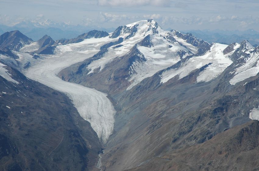
The Austrian Alps have been selected as a study area, because they are at a latitude that is regularly
observed by both GEDI and ICESAT-2, high quality Digital Elevation Models are freely available, and
significant mass loss of the glaciers has been known to occur [7].

The main research question for this master thesis is defined as:

How can a combination of ICESAT-2 and GEDI data be used to detect changes of Alpine glaciers?

This will be further split up between the following sub-questions:

 1. Why is Alpine glacier change relevant?
 2. What is a suitable workflow to process ICESAT-2 and GEDI data to ice thickness changes?
 • How are ICESAT-2 geolocated photon and GEDI geolocated waveform products created
 and how do they compare?
 • How does a combination of ICESAT-2 and GEDI improve the spatial and temporal
 coverage for the selected Alpine glaciers?
 • How can Lidar altimetry be used in combination with a Digital Elevation Model to
 estimate ice thickness changes?
 • What is the quality of estimated ice thickness changes?
 3. How can characteristic features (such as elevation, slope, proximity to the edge of the
 glacier) of locations on the glacier be created and how do they correlate with their estimated
 ice thickness change?
 4. Can estimated ice thickness changes be used to infer the mass balance of the whole glacier?
 5. How do the results compare to those obtained by other methods?

 Figure 1: Kesselwandferner [8]

 8

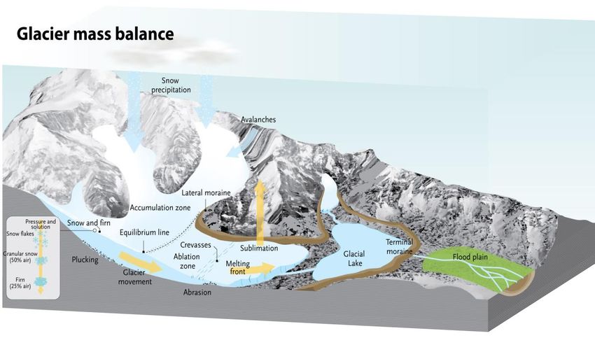
2. Glacier Change Observations

In this chapter an introduction will be given on glacier change observations. Firstly, the morphology
of glaciers will be described, which gives insight into what glacier changes may be expected in
Austria. Secondly, the general types of methods for monitoring glacier changes will be described, and
finally an overview of satellite sensors suitable for glacier studies will be given.

2.1 Glacier Morphology

The spatial distribution of ice loss within a mountain glacier is intrinsically linked to the glacier
structure. Larger glaciers are generally separated into an accumulation zone and an ablation zone by
the equilibrium line, as shown in figure 2. The accumulation zone is the high elevation area where
snow is collected over years and compressed into firn and ice. The ablation zone is the low-lying
glacier tongue where ice flows into the area and is subsequently melted or sublimated. Factors
including the mean glacier elevation, slope of the glacier tongue, debris cover, and avalanche
contributing area all influence the glacier mass balance [9]. The largest examples of this type of valley
glacier in Austria are the Hintereisferner and Gepatschferner in the Ötztal in Tirol, and the Pasterze
glacier in Carinthia.

A distinction is made between glacier retreat, where the extent of the glacier decreases, and glacier
thinning. Glacier retreat significantly alters the geometry of the glacier, and therefore also its ice
mass fluxes. Even glaciers located in the same region which are subject to the same climate and
weather conditions can react differently to climate change due to differences in their morphology
[10]. The mass balance of a glacier is impacted immediately by changes in climate but can take
decades or centuries to reach a new steady state [11].

 Figure 2: Glacier morphology and mass balance components [12]

 9

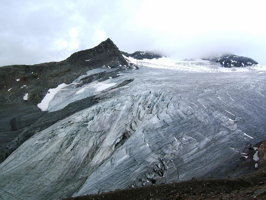
In addition to the well-defined valley glaciers described in figure 2, many smaller patches of
permanent ice exist in Austria. The smallest types of glaciers often have little to no internal ice flow,
which is why they are sometimes called ice patches instead. The glacier inventories used in this study
do not differentiate between different types of permanent ice, and their mass changes are just as
relevant, so they are included in the analysis nonetheless.

Small glaciers can be divided in types that are the remains of a larger glacier (in which case they can
be called glacierets) and types that are simply smaller areas where snow and firn has accumulated
over time [13]. The Austrian glaciers have retreated significantly since the little ice age, and as a
result the smaller types of remaining glaciers are relatively common [14].

Cirque glaciers occur in cases where the glacier tongue has receded so far that only the upmost of
the old accumulation zone remains, often in a circular shape. Smaller ice masses that occur on steep
mountain sides are often called hanging glaciers, cliff glaciers or apron glaciers. Hanging glaciers can
show mass loss through avalanches caused by structural instability, which may take place even if no
melting is taking place [15]. In general, smaller glaciers tend to react more quickly to changes in
temperature or snowfall [14].

 Figure 3: Hallstatter Glacier [16]

 10

2.2 Monitoring of Glaciers

Three general methods exist for the estimation of mass loss of glaciers: glaciological surveys,
gravimetry and altimetry. All three techniques are in some way limited in their spatial and temporal
range and resolution, as well as their accuracy.

Glaciological surveys commonly measure a number of meteorological, geometric and mass balance
characteristics such as glacier runoff, precipitation on the glacier and the surface area of the glacier
[2]. They are limited mainly due to practicality. Only a limited number of glaciers can be measured,
and of those only a limited area, so a large amount of extrapolation is required. However, they have
the advantage of multiple decade long time series for a number of relatively easily accessible
glaciers, such as the list of reference glaciers maintained by the World Glacier Monitoring Service.

Gravimetry involves mapping changes in the earth’s gravity field. These changes correspond to large
movements of mass in the earth’s system. When correcting for other significant signals (such as
glacial isostatic adjustment, hydrology, atmosphere, earthquakes and volcanic activity) changes in
gravity can be used to determine ice mass loss on a large scale. However, it cannot be used for
individual glaciers or smaller regions because it has limited spatial resolution [17].

Altimetry measurements are distinguished by their platform (airborne or spaceborne) and method
(Radar, photogrammetry or Lidar). Airborne altimetry has a higher resolution and accuracy than can
be reached by spaceborne sensors, but has practical limits in terms of price and accessibility so that
only a small number of glaciers will be measured in this way a limited number of times. Spaceborne
Lidar sensors only collect measurements on narrow paths on the ground, essentially creating profiles
of the surface. This is the main disadvantage of spaceborne Lidar measurements for glaciers: glaciers
will be measured a limited number of times (or not at all), and the measurements are only dense in
one direction. Combining different satellite Lidar sensors would increase coverage, which would be
greatly beneficial.

Many studies combine glaciology, gravimetry and altimetry results to arrive at estimates for long
term trends and large scales, e.g. [2] [7].

The general focus of remote sensing glacier mass balance studies has been the contribution of
glaciers to global sea level ice, for which the combined ice loss of a large region is most important.
However, the behaviour of individual glaciers is also of interest, since this can give more insight into
how they react to climate change, which allows for more accurate modelling and prediction of future
ice melt. In addition, glacier changes are not entire homogeneous over a mountain region, and the
behaviour of individual glaciers can be important for local hydrology, ecology and tourism. Accurate
height change measurements are important for the study of the interplay between mass balance,
morphology and climate change [18].

 11

2.3 Satellite Sensors for Detecting Glacier Change

Some of the missions commonly used for similar types of studies include: SRTM, ASTER, GRACE-FO,
ICESAT, TanDEM-X and CRYOSAT-2. Their methods and performance will be summarised here.

An overview of the sensor properties as described in this chapter is given in the table below. It should
be noted that the accuracy of these sensors is often variable, and the values shown in this table are
only a rough indication of the performance over mountainous terrain.

 Accuracy
 Timespan Resolution (approximate) Data availability
SRTM February 2000 30 m 10 m Free

ASTER February 2000 - present 30 m 30 m Free

GRACE(-FO) March 2002 - October 2017, 100's of km N/A Free
 May 2018 – present
ICESAT January 2003 - February 2010 172 m 1m Free

TanDEM-X June 2010 - present 12 m 4m Partly free, partly via proposal

Cryosat-2 April 2010 - present 400 m 40 m Free

 Table 1: Overview of satellite sensor properties

2.3.1 SRTM
The Shuttle Radar Topography Mission (SRTM) was a mission flown in February 2000 with the Space
Shuttle Endeavor to create a Digital Elevation Model (DEM) with near global coverage, using X-band
and C-band Synthetic Aperture Radar. SRTM is widely used in studies of glacier mass changes [19]
[20] [21] [22], for its large coverage, good resolution and because its age results in relatively long
timespans with new data, which results in a better image of the average annual mass change. It has a
resolution of 1 arcsecond, corresponding to 30 m. The accuracy standard of SRTM was set at 16 m
absolute vertical accuracy with a 90% confidence [23]. SRTM is freely available via the EarthExplorer
website of the U.S. Geological Survey.

Accuracy assessment of the SRTM-GL1 DEM shows a standard deviation error of 6.6 m, but there is a
heavy dependence on the slope of the terrain, pointing to a large horizontal error. Areas with a slope
higher than 20 degrees show a standard deviation error of 14.9 m [24]. As can be seen in figure 31 in
chapter 5.2, the Austrian glaciers commonly include slopes much steeper than that, so this should
always be considered when using SRTM data.

The suitability of SRTM for determining glacier heights is controversial. Some results have shown
large disagreements with other methods, likely due to the bias introduced by penetration of the
radar signal in snow and ice, and the uncertainty of applied corrections for this bias [25] [26]. The
depth of radar penetration can be in the order of meters, but depends on the physical properties of
the snow and ice, which are often largely unknown. If no correction is applied, the glacier height in
the SRTM will be underestimated, which also leads to an underestimation of the mass change.

 12

A common solution is to apply a correction based on the elevations found in the study area,
assuming that low lying areas will contain the bare ice of the ablation zone and high areas will
contain loose snow of the accumulation zone. No correction is applied for areas with elevations
below the equilibrium line, and a linearly increasing correction is applied for any areas above it [21]
[22]. However, determining the suitable magnitude of this correction can be difficult since it depends
on the local conditions at the time of data collection. The significant inconsistencies between results
as pointed out by Berthier et al. (2018) were explained by a disagreement between penetration bias
corrections [25].

Dussaillant et al. (2018) finds that SRTM C-band penetration is only an issue for about 1% of the area
of the Northern Patagonia Icefield due to the relatively wet glacier conditions at the time of SRTM
collection [27]. However, for any glaciers in the Northern Hemisphere the SRTM was collected
around the coldest time of the year, and therefore at the most susceptible to radar penetration.

A comparison of the C-band and X-band DEM’s of SRTM could give an indication of the penetration
depth of the study area [28]. This assumes that there is no penetration for the X-band, however it
has been found that X-band penetration can still reach several meters under certain snow and ice
conditions [25]. Only comparing data from the same time of year using the same radar frequency is
another approach to reduce bias [29], assuming that glacier conditions will be relatively similar.

2.3.2 ASTER
ASTER (Advanced Spaceborne Thermal Emission and Reflection Radiometer) is an imaging sensor
aboard the Terra satellite and has been active since February 2000. DEM’s can be created from
ASTER using stereo-photogrammetry. The AST14 DEM product is automatically generated this way
for any location for every 16 day ASTER repeat. This product has a 30 m resolution and a vertical
accuracy ranging between 15 and 60 m depending on the terrain [30]. The ASTER GDEM product is
generally not used for glacier mass change calculations since it is created from a composition of
ASTER images acquired over the mission’s lifetime. ASTER data products are available freely through
NASA Earthdata search.

2.3.3 GRACE
The Gravity Recovery and Climate Experiment (GRACE) mission was launched in 2002 and was the
first satellite mission dedicated to mapping changes in the earth’s gravity field. It finished its mission
in October 2017, and Its continuation GRACE-FO was launched in 2018.

Spaceborne gravimetry is mostly applicable for larger regions with significant mass loss and not for
individual glaciers or subregions due to its low resolution and the need to correct for other mass
change signals (such as glacial isostatic adjustment and hydrology), which is more challenging on a
smaller scale. The filtering methods used to process GRACE and GRACE-FO data result in a spreading
out of the mass signal over many kilometers. As a result, analysing a subset of glaciers in an area will
result in a large amount of signal from neighbouring glaciers leaking in. The spatial resolution of
GRACE data is somewhat subjective as it depends on the post-processing strategy, but is in the order
of hundreds of kilometers [17].

 13

An advantage of the gravimetric approach compared to lidar is that it measures mass changes
directly, so it does not rely on an assumption about ice density. GRACE and GRACE-FO provide a
complete global image monthly, allowing for a complete time series without irregularities for the
entire mission duration. Mass changes caused by atmospheric movement and hydrology are included
in the signal, but cloud coverage is not an issue for gravimetry.

2.3.4 ICESAT
The Ice, Cloud, and Land Elevation Satellite (ICESAT) was the predecessor of ICESAT-2 active from
January 2003 until February 2010. It carried the Geoscience Laser Altimeter System (GLAS),
measuring the surface at a 172 m along-track resolution with a 70 m footprint. ICESAT data is
available via the National Snow & Ice Data Center (NSIDC) website.

Moholdt et al (2010) found a one sigma vertical accuracy of 0.66 m at slopes under 5 degrees in
Svalbard by analysing crossover locations [31], with the accuracy depending heavily on the terrain
slope.

While ICESAT provided a good accuracy, it lacked in terms of resolution, footprint and coverage,
which can be an issue for measuring relatively small mountain glaciers. ICESAT-2 improved upon the
first mission in all these aspects, as will be described in chapter 3.

2.3.5 TerraSAR-X and TanDEM-X
TanDEM-X is a 2010 add-on to the TerraSAR-x mission that allows for the creation of DEM’s from
bistatic radar interferometry. The name TanDEM-X or TDX is also used to refer to the two satellites
combined. Height differences can be determined by either creating a DEM from a single TDX pass
and comparing it against another DEM, or by directly comparing two interferograms created at
different times. As the name implies, the sensor uses the X-band of the radar spectrum, and is
therefore less susceptible to radar penetration bias than the C-band SRTM DEM which was created
with a longer wavelength. TDX has a ground resolution of 0.4 arcseconds or approximately 12 m [32].

Globally, the TDX DEM has a vertical accuracy of 1.09 m [33]. However, like most altimeters the
accuracy decreases for mountainous terrain due to horizontal geolocation errors. Malz et al. (2018)
finds an accuracy of 3.14 m when comparing TDX to SRTM in Patagonia [21]. Sommer et al. (2020)
found a standard deviation of 4.87 m using a similar method in the Alpes [22], and Neckel et al.
(2013) determined an error of 3.70 m in the Himalaya [29]. Neckel et al. also calculated height
differences by directly comparing interferograms of TDX and SRTM, which improved the accuracy to
2.38 m. These accuracy assessments were all performed on non-glacier areas, so radar penetration
bias is not included. The TDX radar penetration bias is in the order of meters depending on glacier
conditions, but can be partially estimated based on the radar backscatter and coherence [34].

TanDEM-X 90 m DEM data is freely available online, whereas higher resolution data products are
accessible via a proposal submission.

 14

2.3.6 CRYOSAT-2
The CryoSat-2 satellite was launched in April 2010 and uses the Synthetic Aperture Radar and
Interferometric Radar Altimeter (SIRAL). Its main mission objectives are to monitor sea ice and to
detect changes on the Antarctic and Greenland ice sheets. Measurement of glacier and ice cap
thickness changes is a secondary objective of the Cryosat-2 mission [35].

CryoSat-2 uses a 2.2 cm wavelength (Ku-band), which is shorter than that of TanDEM-X and SRTM,
which reduces the radar penetration bias [19]. The sensor uses three different modes, of which the
synthetic aperture interferometric (SARIn) mode is used when the satellite crosses any area
containing mountain glaciers or the edges of ice sheets and ice caps, including the Alpes [35]. The
sampling of CryoSat-2 in SARIn mode tends to cluster towards higher elevations, meaning that valley
glaciers can be under-sampled [36] [37]. The Cryosat-2 effective resolution in SARIn mode is
approximately 400 meters with some variation depending on the terrain [38]. Accuracy analyses of
SARIn data over Antarctica and Greenland show that the accuracy decreases rapidly with increasing
terrain gradients. For slopes under 1 degree the random error when compared with ICESAT-1 data is
below 5 m, but for the more mountainous coastal area of Greenland this becomes 40 meters [36]
[39]. Cryosat-2 has also been used successfully for mass loss studies of ice caps in Patagonia, Svalbard
and Iceland [19] [40] [41].

Cryosat-2 has a good spatial coverage, temporal resolution and accuracy over flat terrains. This
makes it especially suitable for analysis of larger ice fields and ice sheets. It has been active since
2010 and has a ground track repeat time of 30 days, allowing for a long and detailed time series
analysis. However, it provides limited and relatively inaccurate data on smaller mountain glaciers
such as those found in Austria. Cryosat-2 data can be accessed freely online via the CryoSat-2 Science
Server of the European Space Agency.

 15

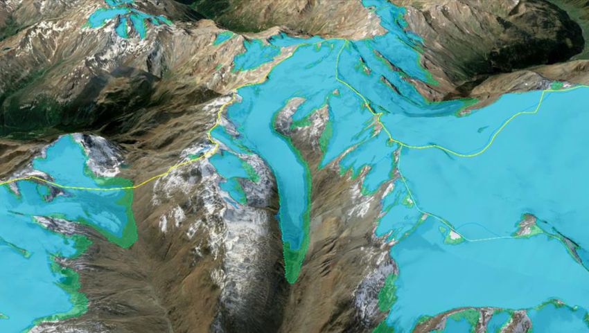
3. ICESAT-2 & GEDI Data Products

Three different altimetry data products were used for this thesis; ATL03 and ATL06 from ICESAT-2
and L2A from GEDI. This chapter gives an overview of these products and of how they are created.
Lastly, the spatial coverage of the lidar ground tracks over Austria will be described.

3.1 ICESAT-2

An overview of the mission characteristics and data products will be given here, followed by a
summarized description of the processing chain from the raw collected data to the land ice surface
heights of ATL06.

3.1.1 Mission overview
The Ice, Cloud, and land Elevation Satellite 2 (ICESAT-2) was launched in September 2018 and carries
the Advanced Topographic Laser Altimeter System (ATLAS) lidar sensor. Like its predecessor its main
purpose is to measure sea ice and ice sheet thickness, which is why it occupies a near polar orbit.
Thanks to this orbit it measures heights globally, so it can be used for many other purposes.

ICESAT-2 has two main conceptual differences compared with ICESAT. Firstly, to improve spatial
resolution ICESAT-2 splits its laser beam into six separate beams, organized in three pairs each
containing a strong and weak beam. The three pairs are separated by 3.3 kilometres, whereas the
strong and weak beams in each pair are separated by 90 meters. This also allows for the cross-track
slope to be measured. In addition, the footprint of the beams is reduced from the 70 meters of
ICESAT to 17 meters for ICESAT-2, and the along-track resolution is increased from 150 meters to 0.7
meters [42]. These improvements are ideal for the sometimes rough surfaces of glaciers, and
potentially allow for more accurate change detection.

 Figure 4: ICESAT-2 ground-track configuration. Six laser beams are used, arranged into three pairs
consisting of a weak and strong beam. The pairs are located 3.3 km apart and the beams within each
 pair are separated by 90 m. The weak beams are always pointed 2.5 km ahead of the strong beams,
 but this has no consequence on the data pattern of data collection [43].

 16

Secondly, it uses a photon-counting lidar instrument called ATLAS instead of ICESAT’s full-waveform
lidar called GLAS. This means that instead of measuring the power of the returned laser beam signal
over time, single returning photons are detected. This change means that the transmitted signal of
the laser could be lowered, which allowed the frequency of the laser beam to be increased while
keeping power requirements limited. This resulted in the much higher along-track resolution [43].
The downside of using photon-counting technology is that the returned signal needs to be
distinguished from the natural background rate of photons.

An overview of ICESAT-2/ATLAS data products is given in figure 5. The data captured by ATLAS is
released in a number of different products to allow different users to select the right location in the
processing chain that best suits their needs. For example, users researching techniques to process
raw space altimetry data can use the ATL00 product, while users only interested in vegetation height
may select ATL08 or ATL18, for which most pre-processing has already been done. The main data
products that are of interest for this research are ATL03 Geolocated Photons and ATL06 Land Ice
Height. ICESAT-2 data is free to download from the National Snow & Ice Data Center website
(nsidc.org).

 Figure 5: ATLAS product processing chain. Data is released as a number of different products to suit
 user needs. The products are grouped by level indicating the degree of processing [44].

 17

3.1.2 ATL00 Telemetered Data
Since ATLAS is a photon counting lidar, it not only detects photons from the transmitted signal, but
also a number of naturally occurring background photons. In order to reduce data size and ensure
that all data can be telemetered some processing steps are done aboard ATLAS for every mainframe,
which are along-track segments of 140 meters.

The ATLAS Flight Science Receiver Algorithms document describes the on-board algorithms that are
used to select data to be telemetered [45]. The photons are initially filtered for a wavelength of 532
nm. For every mainframe a range of elevations is determined where the surface could realistically be
located. This is done based on on-board datasets. Firstly the minimum and maximum elevation of the
approximate location of the mainframe are taken from a Digital Elevation Model. This range is
vertically extended by 250 meters and used to create a first selection of photons. A histogram is
made of this selection, and the bin with the largest amount of returns is assumed to be
approximately at the surface. A Digital Relief Map is used to determine the number of bins above and
below to be added based on the variability of the elevation in the area. As a consequence, a larger
amount of background photons are telemetered for high-relief areas.

By design, a wide margin of background photons is present to ensure that all surface photons are
preserved. Figure 6 shows an along-track profile of a single beam over the Austrian Alpes with all
telemetered photons. While the data in this figure is from the ATL03 product, it shows the typical
amount of photons telemetered in the ATL00 product.

Figure 6: A segment of unfiltered ATL03 data over Austria, showing the vertical extent of telemetered
 photons.

The rate of background photons is not constant, but depends on the solar elevation angle and the
top of atmosphere reflectance of the surface. In order to determine the background rate, an
atmospheric histogram is also made and telemetered for every mainframe.

 18

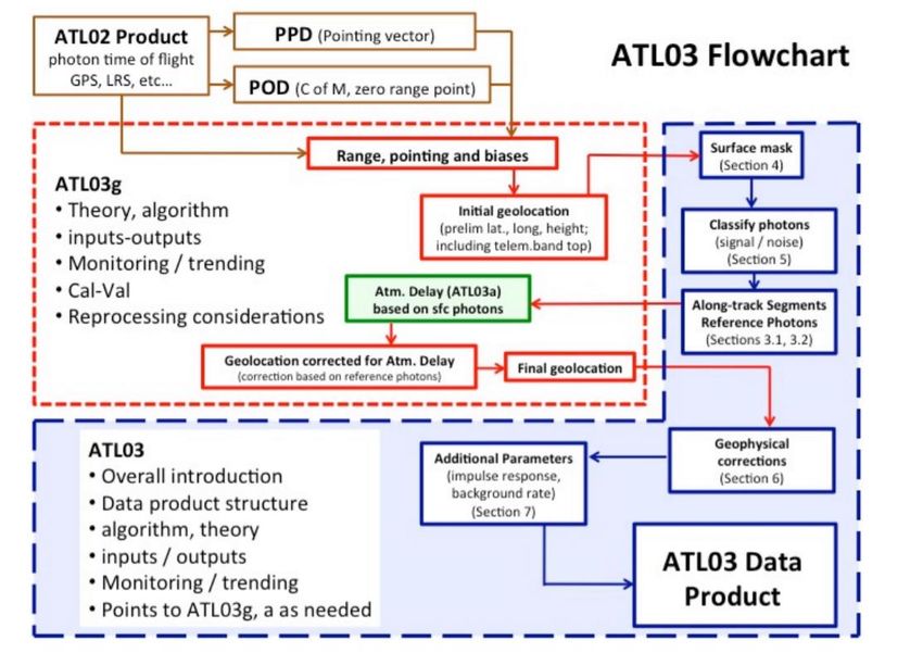
3.1.3 ATL01, ATL02, POD and PPD
After the telemetered data is received, it is time ordered and reformatted into Hierarchical Data
Format (HDF) files and released as the ATL01 reformatted telemetry data product [46]. For the ATL02
data product the time of day (TOD) of the transmitted laser pulses is corrected for biases and
converted to GPS time, and the time of flight (TOF) of all the detected photons relative to the start of
the laser pulse is determined [47]. It also provides radiometric parameters such as the transmitted
energy and the receiver sensitivity.

The algorithms for the precise location of the satellite as a function of time are described separately
in the Precise Orbit Determination (POD) algorithm theoretical basis document, [48]. The direction of
the pointing vector of ATLAS is also derived separately in the Precision Pointing Determination (PPD)
algorithm theoretical basis document, [49]. ICESAT-2 uses a combination of stellar tracking and
inertial reference units to achieve this. The TOF, POD and PPD parameters are the building blocks
that are combined to calculate the geolocation of every photon.

3.1.4. ATL03 Geolocated Photons
The ATLAS algorithms are described in more detail in the ATL03 Algorithm Theoretical Basis
Document (ATBD), [50]. The ATL03g ATBD gives a more detailed description of the geolocation
algorithm, [51]. An overview of the algorithm steps to derive the geolocation of photons is given in
figure 7, where the red bordered area shows the steps described in the ATL03g ATBD.

 Figure 7: ATL03 geolocation algorithm overview. [50]

Firstly, the TOF of the photons is used to calculate the rough range of every photon bounce point
from the instrument. The speed of light in a vacuum is used, and no corrections for atmospheric
delay are applied yet. The range bias at the instrument is constantly monitored by directing a small
portion of the transmitted laser beam directly back into the sensor. This bias is already applied here.

 19

This range is then combined with the POD and PPD parameters to derive the approximate location of
the bounce point on earth. The location is initially derived in the Earth-centred Inertial reference
frame and is then converted to the longitude, latitude and height coordinates of the WGS 84
reference system, with ellipsoidal height.

After this initial geolocation the photons are grouped by their surface type. This is done because
certain parameters in the subsequent photon classification algorithm are adjusted based on surface
type. The used surface types are: land, ocean, sea ice, land ice and inland water. The final purpose of
the surface types is to reduce the amount of data that is passed on to the surface specific level 3
algorithms.

The surface type masks are made from a list of external sources. For the glaciers in Austria, the
relevant source is the Randolph Glacier Inventory (RGI) version 5.0 [52]. More information about the
RGI is given in chapter 4.1 . To ensure that all land ice is captured completely within the surface type
mask, a 10 km buffer is added to the RGI. This also means that the surface type cannot be used to
select only glacier photons, and that photons commonly belong to multiple surface types.

 Figure 8: Surface mask for 'Land Ice' type used by ATL03 [50]

The next step is to classify the photons by their likelihood of being a surface return vs being a
background photon. As shown in figure 6, all telemetered data is present in ATL03, resulting in a thick
layer mostly consisting of background photons. In order to make a distinction between signal and
background a system of quality flags is introduced. This distinction is based on a difference in density
that is introduced by the addition of surface photons in a constant stream of background photons. In
addition, this classification is used to select reference photons for which the atmospheric path delay
is computed. The meaning of the quality flags is shown in table 2.

 20

Quality Flag Confidence Signal to Noise Ratio
0 Background -
1 Background, but added as Buffer -
2 Low SNR < 40
3 Medium 40 < SNR < 100
4 High SNR > 100

 Table 2: ATL03 quality flags

The photon classification algorithm starts by dividing the photons in along-track segments using a
predefined time difference ∆Time. For every ∆Time segment a vertical histogram is made with a bin
size of δz. If the number of photons in any of the bins exceeds the threshold value, all the photons of
that bin are flagged as surface photons. The threshold value is defined as:

 ℎ = µ _ _ + 3 _ _ (1)

Where µ _ _ is the mean background rate of photons adjusted for the bin size and _ _ is
the standard deviation of the background rate adjusted for the bin size. Both values are calculated
from the atmospheric photon histogram that is created for every along-track segment of 140 m.

In the case that no histogram bins are found to have an amount of photons larger than the threshold,
the bin size δz is increased stepwise until either the threshold is satisfied or the maximum vertical bin
size is reached. When the maximum vertical bin size is reached, the along-track width of the
histogram δt will also be increased stepwise until the maximum along-track histogram width has
been reached. If bins containing surface photons have been found using an increased δt only the
photons within the original histogram width ∆Time will be tagged as being surface photons.

In this initial approach the histograms are all created perpendicular to the earth’s reference ellipsoid.
However, in the case of a steep slope the surface photons will be spread out vertically so that the
threshold cannot be reached for any bin size. For this reason the slope is estimated for the remaining
gaps based on any surrounding segments for which surface bins are detected. A new histogram is
made that is perpendicular to this slope, and the previously described process of bin size adjustment
is repeated. In the case that the terrain is very rough and unpredictable the new histogram
orientation may still be unable to resolve, so as a last resort a number of other orientations are tried.

To further classify the surface detection the signal to noise ratio of any surface bin is calculated as
the number of photons contained in it divided by the current mean background photon ratio
µ _ _ . Table 2 shows how the SNR translates to the quality flag. Algorithms for level 3A data
products commonly require a minimum vertical span of photons, so the quality flag with value 1
indicates background photons that are added purely for this requirement.

All predetermined variables used in the algorithm described above are different based on the surface
type and whether the track belongs to a strong beam or a weak beam. Therefore, a single photon can
have different quality flags if it belongs to multiple surface types. Most importantly the minimum
vertical bin size for the land ice surface type is 0.7 m for the strong beam and 0.8 m for the weak
beam, showing that the surface is not perfectly resolved but a range of photons remains.

 21

After classification the photons are binned in predetermined 20 meter along-track segments. For
every segment a single reference photon is selected that has the highest possible quality (quality flag
4 if available) and lies as close as possible to the centre of the segment. The atmospheric path delay
correction is then computed only for the reference photon [53].

The atmospheric path delay is a function of the air density along the path through the atmosphere
taken by the signal. This density depends on the air temperature, atmospheric pressure and the
water vapour partial pressure. Only the variation in water vapour is considered, since variations in
other atmospheric components such as ozone have an insignificant effect. The ATL03 algorithm takes
the necessary atmospheric parameters from the GEOS FP-IT numerical weather model, created by
NASA’s Global Modeling and Assimilation Office. This model has a temporal resolution of three
hours, a 0.3125° longitudinal resolution and a 0.25° latitudinal resolution [54].

The resulting atmospheric path delay correction is applied to the whole segment belonging to the
reference photon. These corrections are normally in the order of several meters. The photons now
have their final geolocation expressed in longitude, latitude and height expressed in the WGS 84
reference system. However, the earth’s land surfaces are not at a constant height, but move in
relatively short timescales as they are subject to large scale forces. These include the tidal forces of
the moon and sun, the shifting weight of the ocean’s due to tides and variations in the Earth’s
rotation and centre of mass. These processes are generally not of interest for users of ATLAS data, so
they are computed for every 20 meter segment and adjusted for by default.

The ATL03 data product files also include the geoid height relative to the reference ellipsoid, taken
from the Earth Gravitational Model 2008, which is determined for every 20 meter segment but not
applied by default.

As of release version 3, ATL03 provides a single, pessimistic estimate of the one-sigma uncertainty of
the geolocation process. This value is 20 meters for the horizontal location, and 0.3 meters for
height. In future releases, the uncertainties will be provided dynamically per reference photon.
However, an estimate in the ATL03g ATBD based on the expected errors in POD, PPD and TOF
products shows that under normal conditions the vertical error will not exceed 0.1 m and the
horizontal error in both along and cross track directions will not exceed 5 m. [51], pp 41.

Figure 9 shows a short segment of the ATL03 data with the highest quality flag over the Austrian
mountains. As can be seen, there is still a number of photons for any given along-track location, and
these photons occupy a range of elevations in the order of meters. This distribution of photons can
have a number of different sources, including:

 - Natural surface roughness at a scale smaller than the resolution
 - Random errors in the geolocation
 - Random errors in ranging, including atmospheric corrections and the distribution of the
 transmitted pulse
 - Variations in height in the cross-track dimension
 - The presence of vegetation

Figure 10 shows how a narrow transmitted pulse is stretched the same way by a rough surface as by
a sloped surface with the same height variation.

 22

Figure 9: Segment of ATL03 data with quality flag 4 over a mountain top in Austria.

 Figure 10: A narrow transmitted pulse is stretched vertically by a surface's roughness and slope [55]

The relevant level 3 data product for glaciers is ATL06: Land Ice Height, which creates a single,
unambiguous surface elevation for any location, but also sacrifices along-track resolution in order to
increase accuracy. All photons with quality flag values one to four are passed on to the higher level
algorithms.

 23

3.1.5. ATL06 Land Ice Elevation
ATL06 transforms the ATL03 geolocated photons into surface heights with an along-track resolution
of 20 m. It works on the assumption that the surface can be approximated as a linear slope on a short
scale. [55]

For every 40 m segment the algorithm selects the group of ATL03 photons that could describe the
surface. For a photon collection of a segment to be considered sufficient the minimal number of
photons must be 10 and the largest along-track distance between photons has to be at least 20
meters. These criteria are first tested with all ATL03 photons with a quality flag larger than 1, which
are classified as surface. If this fails, the added buffer of photons with quality flag 1 as shown in table
2 are added.

For every valid segment, an initial linear slope is fitted with least squares to all available photons. A
rough initial vertical window is created based on the quality of the photons and their spread in the
segment. The algorithm then iteratively reduces the window size using the following steps:

 1. Create a least-squares fit based on all photons within the current window
 2. Calculate all the residuals of the photons, and determine the standard deviation of the
 residuals, corrected for the expected ratio of background photons to surface photons. Also
 calculate the expected spread of photons based on the formula described below with zero
 roughness (R=0)
 3. Define a new window height defined as the maximum of the following:
 a. 6 times the standard deviation of the residuals
 b. 6 times the expected standard deviation based on equation 1
 c. 0.75 times the last window height
 d. 3 meters
 4. Return to step 1 unless the amount of iterations exceeds 20 or the window refinement has
 not resulted in a change of photon selection

The vertical spread of photons for any location (such as shown in figure 9) is estimated by the
formula:
 1
 2
 2
 2 2 (2)
 = [ + ( ) + ( ) ]
 8 2 

Where is the expected vertical standard deviation of photons, is the standard deviation of the
transmitted pulse, W is the footprint diameter, c is the speed of light in a vacuum, is the local
surface slope angle and R is the root mean square deviation from the surface [56]. This estimation is
used in step 2 and 3 of the iterative process to ensure the window size is not reduced too drastically.

 24

Figure 11: ATL06 window height reduction [55]

After the surface window has converged some bias corrections are applied. The difference between
the mean and median photon height in the window is examined to apply a correction for the effect
of outliers. A correction is also applied for the ‘first photon effect’, which takes place when two
photons arrive at the ATLAS sensor with a very small time difference between them. The sensor is
unable to make a distinction between the two and only the first photon will be detected. Therefore,
a slight positive bias is expected when a large group of photons is considered, such as in the 40 meter
segments of the ATL06 algorithm. Lastly, the transmitted pulse of ATLAS is not perfectly symmetric,
but has a trailing edge, also resulting in an offset when considering larger groups of photons. All
these biases are estimated for every segment, and applied to the surface height by default.

ATL06 provides two different uncertainty estimate parameters. The parameter h_li_sigma
propagates the ranging error of the ATL03 photons in the least squares fit. The parameter
sigma_geo_h takes the ATL03 geolocation error and calculates the vertical error caused by this shift
assuming the determined slope is constant. As mentioned for ATL03, the geolocation and ranging
errors are not yet determined dynamically for the data product version 3. A constant and rather
pessimistic value is given instead. These values are propagated for the ATL06 uncertainties, meaning
they reach quite large values, in the order of tens of meters for sigma_geo_h.

A new quality flag is made for ATL06 which indicates if the surface point has failed any of a number
of quality tests. This includes information about the surface window detection, the signal to noise
ratio and the size of residuals. Points with a quality flag of 0 are considered to be of high quality.

Figure 12 shows a comparison of ATL03 data of quality flag 4 and ATL06 data over the Hintereisferner
glacier. The ATL06 heights indeed seem robust to outliers in ATL03. ATL03 seems to include the
presence of crevasses in the glacier, while ATL06 represents the top surface.

 25

Figure 12: (a) ATL03 with quality flag 4 and ATL06 for the left strong beam, (b) ATL03 with quality flag
4 and ATL06 for the right weak beam, (c) location of the data on the Hintereisferner outline from RGI.

 26

3.2 GEDI

An overview of the GEDI mission will be given here, followed by a description of the algorithms used
to create the L1B and L2A data products.

3.2.1 Mission Overview
The Global Ecosystem Dynamics Investigation (GEDI) is a Lidar sensor that was launched in December
2018 and attached to the International Space Station. Its main objective is to observe Earth’s forests
vertical structure and by extent their biomass [57]. GEDI uses a full waveform Lidar to capture the
height and density of vegetation. It splits three lasers into 8 ground tracks, spaced 600 meters apart
in the cross-track direction. The beams have a footprint of approximately 30 meters, and samples are
spaced 60 meters apart in the along-track direction.

 Figure 13: GEDI beam configuration [58]

GEDI data can be freely downloaded from the website of the Land Processes Distributed Active
Archive Center (lpdaacsvc.cr.usgs.gov). The data products that will be used are L1B: ‘Geolocated
waveforms’ and L2A: ‘Ground elevation, canopy top height, relative height (RH) metrics’.

3.2.2 L1B Geolocated Waveforms
GEDI’s full waveform technique means that it does not detect individual photons, but simply
monitors the combined energy of all photons received from the surface. The return of the laser beam
is easily detected over the background noise, and it is time tagged and passed on to the waveform
processing and geolocation algorithms. In addition, the transmitted waveforms are also recorded and
time tagged. The waveforms are recorded at a resolution of 1 ns, corresponding to a 0.15 m vertical
resolution on the ground.

The L1B data product contains the geolocated waveforms. Since the waveforms are not necessarily
perpendicular to the surface, the first and last bin of every waveform are geolocated, allowing the
locations of any of the middle bins to be interpolated if necessary. The geolocation algorithm is
described in [59].

 27

The first step in the geolocation algorithm is to characterize the transmitted pulse, fitting a Gaussian
curve and setting its centre as the start of the transmit time. This allows the time of the received
pulse to be taken relative to the transmitted pulse, which is used to determine the range to the
bounce point.

GEDI uses a combination of GPS and star tracking to determine its location and pointing. The location
and pointing are used with the travel times of received waveform to determine the bounce point of
the first and last waveform bin. The bounce points are converted from GEDI’s inertial reference
frame to the WGS84 system. The atmospheric path delay is then determined using the exact same
method as described for ICESAT-2, which algorithmic basis document is also named as the source for
GEDI [53].

 Figure 14: Example of GEDI (a) transmitted and (b) received waveforms

The L1B product dynamically estimates the uncertainty of its geolocation and height. The height
error estimation ranges approximately between 0.2 and 0.8 meters and the horizontal errors range
between approximately 2 and 11 meters.

Similarly to ICESAT-2, GEDI corrects for solid earth tides, ocean loading and geocenter motion by
default and supplies the geoid height relative to the reference ellipsoid.

3.2.3 L2A Ground elevation, canopy top height, relative height (RH) metrics
The L2A data product contains the elevation of detected surface returns from the geolocated
waveforms. It has the same 60 meter along track resolution as the L1B product.

GEDI was designed specifically for the determination of canopy heights relative to the terrain.
Therefore, the algorithm for the L2A product determines not only the height of the terrain at the
bounce point, but accounts for any number of surface returns above it.

The received waveform interpretation algorithm [60] starts by applying a convolution with a
Gaussian curve for smoothing. The extent of all possible returns is then determined by taking the
segment which is significantly above the background noise level. Inside of this extent, all locations
where the first derivative of the smoothed curve passes zero are tagged as ‘modes’, which are
possible surface returns. Figure 16 shows a sample of GEDI L2A data over the Hintereisferner.

 28