Policy Scenarios for the Revision of the Thematic Strategy on Air Pollution - IIASA
←
→
Page content transcription
If your browser does not render page correctly, please read the page content below
Service Contract on
                             Monitoring and Assessment
                     of Sectorial Implementation Actions
                                (ENV.C.3/SER/2011/0009)

                          Policy Scenarios
                                             for the
                              Revision of the
                 Thematic Strategy on
                                  Air Pollution

                                         TSAP Report #10
                                               Version 1.2

                                                   Editor:
                                           Markus Amann
International Institute for Applied Systems Analysis IIASA

                                              March 2013
The authors
This report has been produced by
         Markus Amann1)
         Imrich Bertok1)
         Jens Borken‐Kleefeld1)
         Janusz Cofala1)
         Jean‐Paul Hettelingh2)
         Chris Heyes1)
         Mike Holland3)
         Gregor Kiesewetter1)
         Zbigniew Klimont1)
         Peter Rafaj1)
         Pauli Paasonen1)
         Max Posch2)
         Robert Sander1)
         Wolfgang Schöpp1)
         Fabian Wagner1)
         Wilfried Winiwarter1)

Affiliations:
          1)
             International Institute for Applied Systems Analysis (IIASA), Laxenburg, Austria
          2)
             Coordination Centre for Effects (CCE) at RIVM, Bilthoven, The Netherlands
          3)
             EMRC, UK

Acknowledgements
This report was produced under the Service Contract on Monitoring and Assessment of Sectorial
Implementation Actions (ENV.C.3/SER/2011/0009) of DG‐Environment of the European Commission.
The modelling methodology that has been used for this report has been updated under the EC4MACS
(European Consortium for the Modelling of Air pollution and Climate Strategies) project with financial
contributions of the LIFE financial instrument of the European Community.
The work by Pauli Paasonen on aerosol number emissions is funded by the Department of Physics of the
University of Helsinki, Finland.

Disclaimer
The views and opinions expressed in this paper do not necessarily represent the positions of IIASA or its
collaborating and supporting organizations.
The orientation and content of this report cannot be taken as indicating the position of the European
Commission or its services.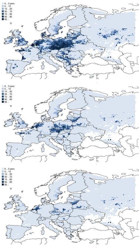
Executive Summary
This report explores how the European Union could make further progress towards the
objectives of the EU’s Environment Action Programme, i.e., to achieve ‘levels of air quality that
do not give rise to significant negative impacts on, and risks to human health and environment’.
It confirms earlier findings that there is still large scope for additional measures that could
alleviate the remaining damage. This scope prevails despite the significant air quality
improvements that emerge from current EU air quality legislation. However, such further
environmental improvements require additional efforts to reduce emissions, which are
associated with additional costs. It is estimated that in 2025 the full implementation of all
currently available technical measures would involve additional emission control costs of up to
0.3% of GDP, compared to 0.6% that are spent under current legislation.
As a rational approach, the report compares marginal costs of further emission reductions
against their marginal benefits. Restricted to monetized benefits of adult mortality from
exposure to PM2.5, marginal health benefits are found to equal marginal costs of further
measures slightly above a 75% ‘gap closure’ between the current legislation baseline and the
maximum feasible reductions. At this level, emission reduction costs (on top of current
legislation) amount to 4.5 billion €/yr, while benefits from these measures are estimated at 30.4
billion €/yr.
However, such a narrow focus on health benefits leaves out ‘low hanging fruits’ for ozone,
eutrophication and acidification that could be achieved at little extra cost. A central scenario is
analysed further that in 2025 would achieve 75% of the possible health improvements, 65% of
the possible gains for acidification, 60% of the potential for less ground‐level ozone, and 55% for
eutrophication. At costs of 5.8 billion €/yr (0.04% of GDP), these measures would cut SO2 by
77%, NOx by 65%, PM2.5 by 50%, NH3 by 27% and VOC by 54% relative to 2005. In addition, BC
emissions would be decline by 33%, particle number emissions by 73% and Hg emissions by 33%.
These measures for 2025 were scrutinized against potential regret investments that would
become obsolete in 2030 if the emission source would be phased out as part of economic
restructuring. It was found that the emission ceilings of the central scenario do not contain
significant regret investments, considering the uncertainties around the baseline projection.
Appropriate flexibility mechanisms could avoid such regret investments for specific situations
where the energy system would drastically restructure.
Numerous uncertainties affect future levels of baseline emissions and the potential and costs for
further measures. A sensitivity case demonstrates the feasibility of the central environmental
targets under the assumptions of the earlier TSAP baseline, which was more optimistic about
future economic development. However, it was found that not all of the corresponding emission
ceilings that have been cost‐optimized for the TSAP‐2013 scenario would be achievable under
the TSAP‐2012 assumptions. It has been demonstrated that alternative sets of emission ceilings
could be derived that could avoid excessive costs to individual Member States if reality
developed differently from what has been assumed in the cost‐effectiveness analysis. However,
such ‘insurance’ against alternative developments comes at a certain cost.
With the current assumptions on costs for low sulphur fuels, the additional costs of packages of
SECAs and NECAs in the 200 nm zones of the EU Member States (with the exception of a SECA in
the Mediterranean Sea) could be almost compensated by cost‐savings at land‐based sources.
Europe‐wide regulations of agricultural emission control measures such as those outlined in the
Draft Annex IX of the revised Gothenburg Protocol could be part of a cost‐effective solution for
achieving the environmental targets of the A5 scenario.

                                                                                                 Page 1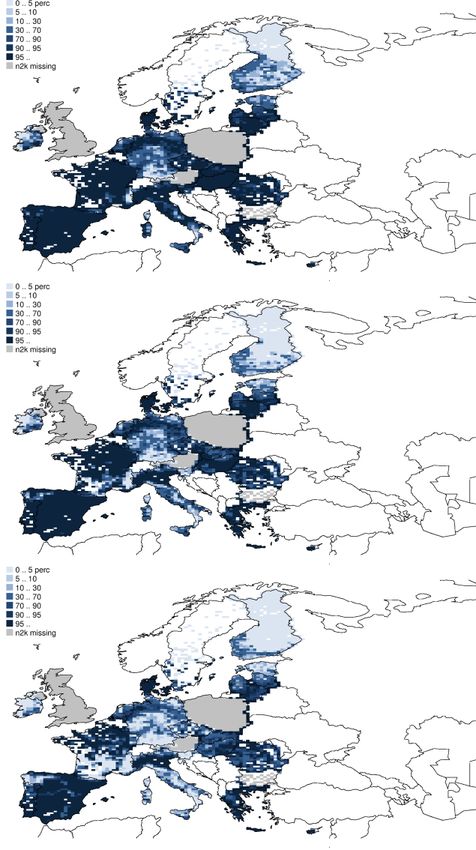
List of acronyms

BAT            Best Available Technology
BC             Black Carbon
bbl            barrel of oil
boe            barrel of oil equivalent
CAFE           Clean Air For Europe Programme of the European Commission
CAPRI          Agricultural model developed by the University of Bonn
CO2            Carbon dioxide
CCS            Carbon Capture and Storage
EC4MACS        European Consortium for Modelling Air Pollution and Climate Strategies
EU             European Union
GAINS          Greenhouse gas ‐ Air pollution Interactions and Synergies model
GDP            Gross domestic product
Hg             Mercury
IED            Industrial Emissions Directive
IIASA          International Institute for Applied Systems Analysis
IPPC           Integrated Pollution Prevention and Control
kt             kilotons = 103 tons
LCP            Large Combustion Plants
NO2            Nitrogen dioxide
NOx            Nitrogen oxides
NEC            National Emission Ceilings
NECA           NOx Emissions Control Area
NH3            Ammonia
NMVOC          Non‐methane volatile organic compounds
NOx            Nitrogen oxides
O3             Ozone
PJ             Petajoule = 1015 joule
PM10           Fine particles with an aerodynamic diameter of less than 10 µm
PM2.5          Fine particles with an aerodynamic diameter of less than 2.5 µm
PRIMES         Energy Systems Model of the National Technical University of Athens
SECA           Sulphur Emissions Control Areas
SNAP           Selected Nomenclature for Air Pollutants; Sector aggregation used in the CORINAIR emission
               inventory system
SO2            Sulphur dioxide
SULEV          Super Ultra‐Low Emission Vehicles; a terminology used for the Californian vehicle emission
               standards
TSAP           Thematic Strategy on Air Pollution
VOC            Volatile organic compounds

     Page 2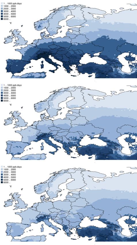
Table of contents
1 Introduction ................................................................................................................................................... 5
1.1 Objective of this report ......................................................................................................................... 5
1.2 Methodology ......................................................................................................................................... 5
1.3 Structure of the report .......................................................................................................................... 5
2 Changes since the last report......................................................................................................................... 6
2.1 Updates of GAINS databases to reflect new national information ....................................................... 6
2.2 The TSAP‐2013 Baseline ........................................................................................................................ 8
2.3 Downscaling methodology .................................................................................................................... 8
2.4 Impact assessment methodologies ....................................................................................................... 8
3 Projections of energy use and agricultural activities ................................................................................... 10
3.1 The draft TSAP‐2013 Baseline ............................................................................................................. 10
3.1.1 The draft PRIMES‐2012 Reference energy projection .................................................................... 10
3.1.2 The 2012 CAPRI scenario of agricultural activities.......................................................................... 11
3.2 The revised TSAP‐2012 Baseline ......................................................................................................... 12
3.3 Comparison of activity data ................................................................................................................ 13
4 The scope for further emission reductions .................................................................................................. 14
4.1 Assumptions on emission control scenarios ....................................................................................... 14
4.1.1 Emission control legislation considered in the ‘Current legislation’ (CLE) scenarios...................... 14
4.1.2 The ‘Maximum technically feasible reduction’ (MTFR) scenario .................................................... 15
4.2 Baseline emissions and scope for further reductions ......................................................................... 16
4.2.1 The draft TSAP‐2013 Baseline ......................................................................................................... 16
4.2.2 Comparison with the TSAP‐2012 Baseline ...................................................................................... 19
4.3 Emissions of non‐EU countries ............................................................................................................ 21
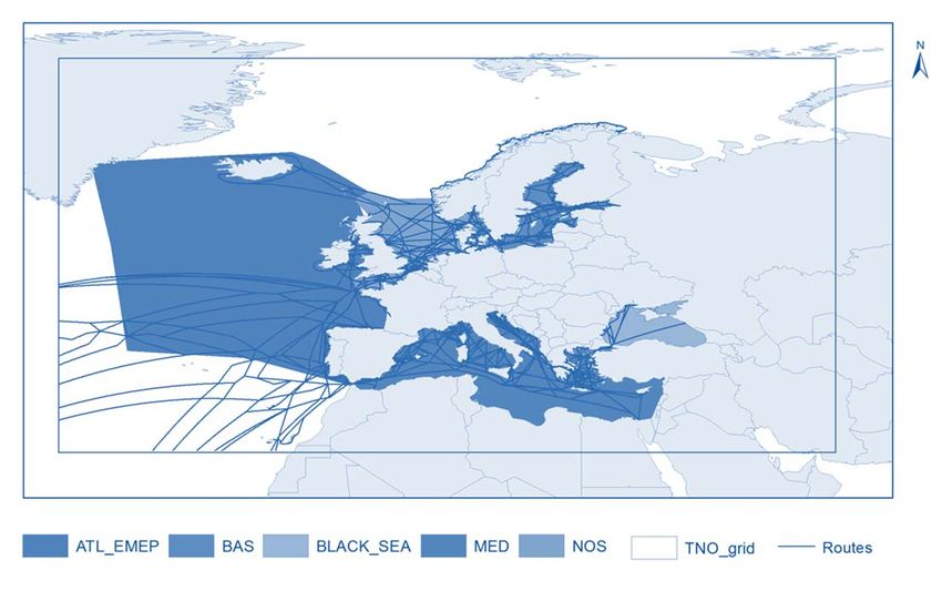
4.4 Emissions from marine shipping ......................................................................................................... 21
4.5 Air quality impacts .............................................................................................................................. 23
4.5.1 Health impacts from PM2.5 ............................................................................................................ 23
4.5.2 Health impacts from ground‐level ozone ....................................................................................... 24
4.5.3 Eutrophication ................................................................................................................................ 24
4.5.4 Acidification of forest soils.............................................................................................................. 26
4.5.5 Compliance with NO2 limit values .................................................................................................. 27
4.5.6 Compliance with PM10 limit values................................................................................................ 28
Page 3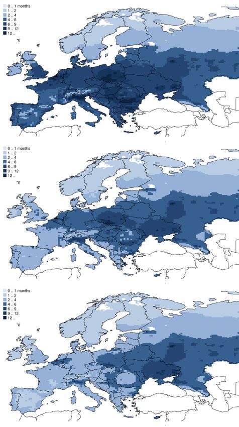
5     Costs and benefits of further emission reduction measures ....................................................................... 30

    5.1       Costs and benefits of measures to improve human health ................................................................ 31

      5.1.1       Cost‐effective emission reductions................................................................................................. 31

      5.1.2       Health benefits ............................................................................................................................... 31

    5.2       Comparison of marginal costs and benefits ........................................................................................ 32

    5.3       Additional targets for non‐health impacts .......................................................................................... 33

    5.4       Feasibility under the TSAP‐2012 assumptions .................................................................................... 34

    5.5       Comparison of emission control costs ................................................................................................ 34

    5.6       Analysis of regret investments ............................................................................................................ 35

6     Options for achieving the environmental targets ........................................................................................ 37

    6.1       The central case (Scenario A5) ............................................................................................................ 37

      6.1.1       Emissions in 2025............................................................................................................................ 37

      6.1.2       Emission reductions by source sector ............................................................................................ 43

      6.1.3       Emission control costs .................................................................................................................... 45

      6.1.4       Air quality impacts .......................................................................................................................... 46

    6.2       Achieving emissions ceilings of the A5 scenario under TSAP‐2012 assumptions ............................... 50

    6.3       Further controls of marine emissions ................................................................................................. 52

    6.4       Europe‐wide measures for agricultural emissions .............................................................................. 53

7     Sensitivity analyses ...................................................................................................................................... 56

    7.1       Impacts of different assumptions on Euro‐6 real‐world emissions .................................................... 56

      7.1.1       Assumptions for sensitivity cases ................................................................................................... 56

      7.1.2       NOx emissions ................................................................................................................................. 57

      7.1.3       Compliance with NO2 limit values .................................................................................................. 58

8     Conclusions .................................................................................................................................................. 60

More information on the Internet
More information about the GAINS methodology and interactive access to input data and results is available at
the Internet at http://gains.iiasa.ac.at/TSAP.

    Page 4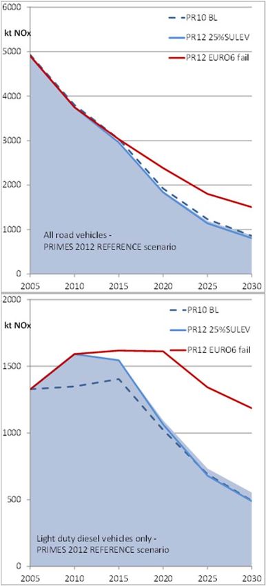
1                Introduction
The European Commission is currently reviewing        project, which was funded under the EU LIFE
the EU air policy and in particular the 2005          programme (www.ec4macs.eu).
Thematic Strategy on Air Pollution. It is envisaged
                                                      The EC4MACS model toolbox (Figure 1.1) allows
that in 2013 the Commission will present
                                                      simulation of the impacts of policy actions that
proposals for revisions of the Thematic Strategy.
                                                      influence future driving forces (e.g., energy
As analytical input to these forthcoming policy       consumption, transport demand, agricultural
proposals, IIASA developed baseline emission          activities), and of dedicated measures to reduce
projections in the TSAP Report #1 (Amann et al.       the release of emissions to the atmosphere, on
2012a), explored their environmental impacts in       total emissions, resulting air quality, and a basket
TSAP Report #6 (Amann et al. 2012b), and              of air quality and climate impact indicators.
presented an initial screening of cost‐effective      Furthermore, through the GAINS optimization tool
additional emission control measures in TSAP          (Amann 2012), the framework allows the
Report #7 (Amann et al. 2012d). This information      development of cost‐effective response strategies
offers now a solid basis for more refined policy      that meet environmental policy targets at least
analyses to identify practical packages of measures   cost.
that could achieve further air quality
improvements in cost‐effective ways.

1.1 Objective of this report
To provide an analytical basis for the Commission
proposal on the review of the Thematic Strategy,
this report explores options for further
improvements of air quality in Europe beyond
current legislation.
                                                      Figure 1.1: The EC4MACS model suite that describes the
The report reviews the potential for environmental    full range of driving forces and impacts at the local,
improvements offered by emission control              European and global scale.
measures that are not yet part of current
legislation, and compares costs and benefits of
cost‐effective packages of measures to reduce         1.3 Structure of the report
negative health and vegetation impacts.
                                                      Section 2 of this report provides a brief summary
The central analysis relies on the new draft TSAP‐    of the changes that have been introduced to the
2013 scenario that incorporates the draft PRIMES‐     modelling methodology and databases. Section 3
2012 energy projection that has been recently         introduces the new draft TSAP‐2012 Baseline
presented to Member States. Key findings are          projection, and Section 4 discusses the scope for
cross‐checked against alternative energy futures,     further air quality improvements beyond the
i.e., against the TSAP‐2012 Baseline that employed    baseline projections. Section 5 explores costs and
the PRIMES‐2010 scenario, which assumed, inter        benefits of additional measures, while Section 6
alia, significantly higher economic growth.           assesses alternative ways for implementation of
                                                      some of the optimized scenarios. Sensitivity
                                                      analyses are carried out in Section 7, and
1.2 Methodology                                       conclusions drawn in Section 8.

This report employs the model toolbox developed
under the EC4MACS (European Consortium for
Modelling of Air pollution and Climate Strategies)

                                                                                                   Page 5
2 Changes since the last report
This analysis constitutes #10 of a series of reports Better match was achieved through adjustments
that assess various aspects that are relevant for a of control strategies and emission factors.
strategic review of the current EU legislation on air
In addition, new information allowed a better
quality. All reports are accessible on the Internet1.
classification of gas use in the power sector, so
Since the last TSAP Report #6 report, (Amann et al. that GAINS distinguishes now four types of plants
2012b), the following changes have been (i.e., plants with boilers, turbines, gas combined
implemented in the GAINS database and to the cycle plants, and gas engines). These categories
GAINS methodology. differ in their emission factors and the potential
for further emission controls. In addition, emission
factors for gas fired power plants have been
2.1 Updates of GAINS databases to updated to better reflect features of individual
countries, such as age and operating regimes. Also,
reflect new national
emission factors for stationary combustion engines
information in the power sector (generators) have been
In the second half of 2012, bilateral consultations revised based on data provided by CITEPA.
were held with 15 countries (Austria, Belgium, Investment costs for refinery boilers and furnaces
Bulgaria, Denmark, Estonia, Finland, France, using heavy fuel oil have been revised to reflect
Germany, Ireland, Italy, Luxembourg, Netherlands, higher capital investments for co‐fired units due to
Sweden, Switzerland, UK). larger flue gas volume). Information was provided
After validation and consistency checks, the new by experts from the refining industry (CONCAWE).
information provided by national experts on The description of legislation on national maritime
energy statistics, emission inventories, emission activities has been refined to include the IMO
factors and the penetration of emission controls MARPOL Annex VI emission and fuel standards as
has been incorporated into the GAINS databases. well as the compromise agreement between the
As the new PRIMES‐2012 scenario was not yet EU Member States, the European Parliament and
available at the time of these consultations, the the European Commission. The latter requires
new information has been applied to the draft implementation of the general sulphur limit 0.5% S
TSAP‐2012 Baseline that relies on the PRIMES‐ already in 2020. SECA legislation has been included
2010 baseline energy projection. Thus, the draft for the Baltic and the North Sea with the English
TSAP‐2012 Baseline presented in this report is Channel.
different from the version introduced in the TSAP
report #6. The new information has also been used In addition, numerous changes for individual
for the conversion of the new PRIMES‐2012 countries were implemented. Some examples
Reference scenario into the GAINS TSAP‐2013 include:
Baseline. Belgium: inclusion of waste fuels in chemical
industry, which are not reported in the
Stationary energy use
EUROSTAT statistics; corrections of control
The, GAINS database was revised to better strategies; update of applicabilities of control
reproduce recent national emission inventories for technologies.
2005 and 2010 as reported to EMEP in 2012. This Finland: inclusion of country‐specific emission
revision took into account the results of bilateral factors for black liquor, modifications of PM
consultations as well as consultations with emission factors for boilers to align with the
industrial stakeholders (EURELECTRIC, CONCAWE). Finnish national inventory.
Germany: revision of data on (bio‐)gas
1
http://www.iiasa.ac.at/web/home/research/researchPr engines, changed structure of brown coal used
ograms/MitigationofAirPollutionandGreenhou
segases/TSAP‐review.en.html
Page 6
for power generation according to the recent categories as well as between non‐road categories
statistics (high vs. low sulphur lignite). for Austria, Finland, Germany, Ireland, Italy, the
Netherlands, Sweden, Switzerland, and the UK.
Estonia: inclusion of characteristics of oil shale
These structural changes have been propagated to
combustion technologies and shale oil
the future scenarios. The fleet composition by
refineries (unique technologies, not used in
technology (in GAINS the so‐called ‘control
other countries).
strategy’) has been cross‐checked with experts
France: revision of emission factors and from these countries and revised where
activity data for combustion and process appropriate. To explore the implications of a
sectors based on detailed inventory by slower turnover of passenger diesel car fleets, a
CITEPA. sensitivity scenario is presented in this report.
Netherlands: changed structure of liquid fuels In addition to country comments, the following
consumption for power generation in CHP changes have been implemented:
plants in refineries (less heavy fuel oil, more
The PRIMES‐2012 Reference scenario has been
other liquid fuels with lower sulphur content);
fully implemented in terms of transport activity
inclusion of emissions from processes in
and associated changes in the fleet. The previously
mineral products industry previously not
used PRIMES 2010 BASELINE scenario is now
properly covered in the GAINS database).
interpreted as a “high economic growth” variant.
Residential combustion PM emission factors for tyre and brake wear have
been revised downwards in the light of recent
Activity data for non‐commercial wood and/or evidence; likewise, NOx and PM emission factors
structure of installations, i.e., shares of stoves, for non‐road mobile machinery have been revised.
boilers, etc. in fuel (both wood and coal) use for Real‐driving NOx emissions from Euro‐6 light duty
past years and future have been provided by diesel vehicles are assumed to decrease in two
Austria, Belgium, Cyprus, Denmark, Estonia, steps, namely to about 310 mg NOx/km in a first
Finland, France, Italy, Poland, Slovak Republic, step and to 120 mg NOx/km in the second step.
Slovenia, and Sweden. Vehicles with these average emissions are
Local measurements of emission factors provided assumed to be introduced from 2014 and from
by Denmark, Finland, Italy, Slovak Republic, UK 2017 onwards in the baseline scenario.
helped to update national emission factors.
Agriculture
Austria, Denmark, Estonia, Finland, Italy, Slovak
Republic, Sweden, and the UK provided new New data on livestock and fertilizer use have been
assessments about the penetration of more obtained from several countries and used to
advanced combustion technologies in this sector, update historical data for recent years and 2010
their future evolution following existing legislation also with respect to number of animals kept on
(certification of new installations), and expected solid and liquid systems and shares of urea in total
replacement rates due to retirement of existing mineral N fertilizer use. The updated information
installations. was also applied to the new CAPRI projections
where such distinction is missing. The above was
Mobile sources done for Austria, Belgium, Denmark, France,
Ireland, Italy, Netherlands, Slovak Republic,
For transport, major improvements relate to fuel
Switzerland, UK.
allocation (diesel/gasoline) across vehicle
categories (heavy/light duty vehicles), emission In the last years, more and more countries have
factors and the penetration of Euro‐standards. This started using the Tier2 methodology of the EEA
now brings the GAINS emission estimate for the Emission Inventory Guidebook for estimating
year 2010 in very close agreement with national ammonia emissions. Beyond that, a number of
inventories. countries committed their own national studies to
analyse the local production conditions, efficiency,
Most importantly, (diesel) fuel has been re‐
and resulting losses of ammonia from agriculture.
allocated between different road vehicle
Page 7
This new information was used to update               Austria, Switzerland and Finland includes now
ammonia emission factors for Austria, Denmark,        agricultural burning. Based on this information and
France, Ireland, Netherlands, UK.                     drawing on results from remote sensing, the
                                                      GAINS database has been revised for Belgium,
Accurate estimates of ammonia emissions, as well
                                                      Bulgaria, Czech Republic, Denmark, Finland,
as other species, require analysis of the policies
                                                      France, Germany, Hungary, Italy, Netherlands,
and their implementation. The implementation of
                                                      Poland, Portugal, Romania, Slovenia, Spain,
mandatory and voluntary measures in agriculture
                                                      Sweden, Switzerland, UK.
has been always a challenge and only recently
more attention has been given to agricultural
emissions to the air.
                                                      2.2 The TSAP‐2013 Baseline
Several Member States (Austria, France, Ireland,
Italy, Netherlands) provided new information on       Compared to TSAP Reports #1 and 6, a new draft
implementation status and management practices        TSAP‐2013 Baseline has been developed. It
that resulted in the development of new emission      employs the most recent draft PRIMES‐2012
factors and assumptions on the penetration of         Reference energy and CAPRI agricultural
specific control measures.                            projections that have been presented for
                                                      comments to Member States in late 2012. Details
VOC emissions                                         of the PRIMES‐2012 scenario are provided in
                                                      Section 3.
A number of countries (Austria, Belgium, Estonia,
Italy, Netherlands, United Kingdom) provided new
information about recent developments in several
industries, which was used to update historic
                                                      2.3 Downscaling methodology
activity data in GAINS and adjust projections for     The new downscaling methodology that has been
future years.                                         developed under the EC4MACS project to estimate
New information on control strategies for solvent     the impacts of future emission scenarios on
use and liquid fuel production and distribution was   compliance with air quality limit values for PM10
provided by Austria, Belgium, Estonia, Ireland,       and NO2 has now been fully implemented in the
Italy, Netherlands, Sweden, United Kingdom.           GAINS model. The methodology is documented in
                                                      TSAP Report #9 (Kiesewetter et al. 2013).
On‐field burning of agricultural residue              After the initial assessment presented in TSAP
                                                      report #6, the AIRBASE monitoring stations have
Following discussion with national experts, SEG4,
                                                      been allocated to the air quality management
groups working on the assessment of open
                                                      zones established under the Air Quality Daughter
biomass burning (including agricultural fires) with
                                                      Directive, so that compliance statistics can now be
remote sensing techniques (i.e., GFED, FINN, and
                                                      evaluated and presented for these zones across
University of Michigan) were contacted to improve
                                                      Europe.
the representation of this activity in GAINS based
on latest available knowledge.
Most recent national reporting documented at          2.4 Impact assessment
www.ceip.at has been used to update the GAINS
                                                          methodologies
estimates; however, many countries do not report
any agricultural burning. This was also confirmed     The HRAPIE (Health risks of air pollution in Europe)
during bilateral consultation where several           project conducted by the European Centre for
national experts confirmed. At the same time,         Environment and Health of the World Health
however, nearly all experts recognized the fact       Organization       has       provided        specific
that most countries have exceptions to the rules      recommendation       of    concentration‐response
and issue occasional permits. Furthermore, the        functions for core input into the GAINS model for
emission inventory community often did not            mortality from PM2.5 and ozone to be used in
investigate the enforcement efficiency of the ban.    cost‐effectiveness analysis (WHO 2013). The
As a consequence, the most recent reporting from      recommendations consider specific conditions of

  Page 8
EU countries, in particular in relation to the range congestive heart failure, and myocardial
of PM2.5 and ozone concentrations expected to be infarction). However, these effects should be
observed in EU in 2020 and availability of baseline treated in sensitivity analyses of the cost‐benefit
health data. assessment.
For fine particulate matter, it is recommended that The above‐mentioned modifications, i.e., the new
the core cost‐effectiveness analysis includes relative risk factors, have been introduced into the
estimates of impact of long term (annual average) GAINS framework that is used for this report. The
exposure to PM2.5 on all‐cause (natural) mortality calculations employ now the most recent mortality
in adult populations (age >30), based on a linear numbers provided in the WHO ‘Health for All’
concentration‐response function, with relative risk database2.
of 1.062 (95% CI 1.040 – 1.083) per 10 µg/m3. The
impacts are to be calculated at all levels of PM2.5.
The central relative risk factor of 1.062 emerges
from the most recently completed meta‐analysis
of all cohort studies published until January 2013
by Hoek et al (Environmental Health 2013, prov.
accepted). 13 different studies conducted in adult
populations of North America and Europe
contributed to estimation of this coefficient. This
factor is slightly higher compared to the factor of
1.06 that has been used for earlier GAINS analysis
based on Pope III et al. 2002.
It is recommended to explore the implications of
alternative, more refined approaches (e.g., cause‐
specific mortality estimates, non‐linear relative risk
functions, etc.) in the context of benefit analyses.
For ozone, the core cost‐effectiveness analysis
should be based on estimates of impact of short
term (daily maximum 8‐hour mean) exposure to
ozone on all‐ages all‐cause mortality. The impacts
of ozone in concentrations above 35 ppb
(70 µg/m3), i.e., using SOMO35, should be
calculated with a linear function with a risk
coefficient of 1.0029 (95%CI 1.0014‐1.0043) per
10 µg/m3 These new coefficients are based on
data from 32 European cities included in the
APHENA study (Katsouyanni et al. 2009). Earlier
GAINS analysis employed a factor of 1.003.
It is noted that after 2005 several cohort analyses
have been published on long‐term ozone exposure
and mortality. There is evidence from the most
influential study, the American Cancer Society
(ACS) study, for an effect of long‐term exposure to
ozone on respiratory and cardiorespiratory
mortality, which for the latter is less conclusive.
Also, there is some evidence from other cohorts
for an effect on mortality among persons with
potentially predisposing conditions (chronic 2
http://www.euro.who.int/en/what‐we‐do/data‐and‐
obstructive pulmonary disease, diabetes, evidence/databases/mortality‐indicators‐by‐
67‐causes‐of‐death,‐age‐and‐sex‐hfa‐mdb.
Page 93 Projections of energy use and agricultural activities
While the earlier PRIMES‐2010 projection has
3.1 The draft TSAP‐2013 Baseline
assumed fast recovery after the economic
A draft version of a baseline projection has been downturn in 2008, the 2012 scenario considers the
developed that employs the latest projections of prolonged stagnation period that has occurred
economic growth, energy use, transport activities since then, and is less optimistic about future
and agricultural production developed by the growth rates. Thus, in the recent scenario GDP in
European Commission. This draft TSAP‐2013 2030 is 7% lower than in the earlier projection.
Baseline combines energy projections of the
Additional differences apply to assumptions on
PRIMES‐2012 Reference scenario and the
energy and climate policies. The draft PRIMES‐
corresponding projections of agricultural activities
2012 Reference projection considers all EU policies
produced by the CAPRI model.
that were adopted by the Commission under
energy, transport, overall economic and climate
trends. It assumes in particular that the national
3.1.1 The draft PRIMES‐2012 Reference targets for renewable energy for 2020 are met.
energy projection
The draft PRIMES‐2012 Reference energy
projection has been presented to Member States Energy use
in late 2012. This projection assesses the impacts
of all EU policies that have been adopted given The assumptions in the draft PRIMES‐2012
current energy, transport, overall economic and scenario on economic development, enhanced
climate trends. energy efficiency and renewable energy policies
and climate strategies lead to almost 10% lower
Key assumptions fuel consumption in 2030 compared to 2005
(Figure 3.2, Table 3.1).
One major difference to earlier scenarios emerges
for the assumed future economic development
(Figure 3.1). 90
Coal
Oil
80 Gas
Nuclear
18 Biomass
PRIMES 2012 Old MS 70 Other renewables
PRIMES 2012 New MS
16
PRIMES 2010 Old MS 60
1000 PJ/yr
PRIMES 2010 New MS
14
50
12
40
Trillion Euro/yr
10
30
8
20
6
10
4
0
2005 2010 2015 2020 2025 2030
2
0 Figure 3.2: Energy consumption by fuel of the PRIMES‐
2005 2010 2015 2020 2025 2030 2012 projection, EU‐28
Figure 3.1: Projections of GDP up to 2030; the PRIMES‐
2012 scenario (shaded area) compared to the The adopted policies for renewable energy sources
assumptions of the PRIMES‐2010 case (lines) (EU‐28, in
are expected to increase biomass use by more
€2005)
than a factor of two thirds in 2030 compared to
Page 102005, and to triple energy from other renewable The projected evolution of energy consumption by
sources (e.g., wind, solar). In contrast, coal Member State is summarized in Table 3.3.
consumption is expected to decline by 40% by Implications for future emissions and the scope for
2030, and oil and natural gas consumption is further emission reductions are explored in
calculated to be 20% lower than in 2005. Section 4.
On a sectorial basis, the rapid penetration of
energy efficiency measures maintains constant or
slightly decreasing energy consumption despite 3.1.2 The 2012 CAPRI scenario of
the assumed sharp increases in production levels agricultural activities
and economic wealth (Figure 3.3, Table 3.2). The CAPRI model has been used to project future
agricultural activities in Europe coherent with the
macro‐economic assumptions of the draft PRIMES‐
90
Power 2012 Reference scenario and considering the likely
Industry
80 Domestic
impacts of the most recent agricultural policies.
Transport The evolution of livestock is summarized in Figure
70 Feedstocks
3.4.
60
180
1000 PJ/yr
Cows and cattle Pigs Chicken
50 Sheep Horses Other
160
40
140
Livestock Units (million LSU)
30
120
20
100
10
80
0
60
2005 2010 2015 2020 2025 2030
40
Figure 3.3: Energy consumption by sector of the PRIMES‐
2012 projection, EU‐28 20
0
2005 2010 2015 2020 2025 2030
New legislation on fuel efficiency should stabilize
the growth in fuel demand for total road transport Figure 3.4: CAPRI projection of agricultural livestock in
despite the expected increases in travel distance the EU‐28 for the PRIMES‐2012 Baseline scenario
and freight volumes. (million livestock units)
Table 3.1: Baseline energy consumption by fuel in the EU‐28 (1000 PJ, excluding electricity trade)
2005 2010 2015 2020 2025 2030
Coal 12.2 10.8 11.6 10.4 9.3 7.2
Oil 28.8 26.7 25.7 24.3 23.6 23.1
Gas 17.7 17.5 17.1 16.1 15.4 14.7
Nuclear 10.3 9.9 9.9 8.3 7.9 9.2
Biomass 3.0 5.1 5.8 6.6 6.6 6.7
Other renewables 2.1 2.7 3.8 5.1 6.0 6.8
Total 74.2 72.7 73.9 70.9 68.8 67.7
Table 3.2: Baseline energy consumption by sector in the EU‐28 (1000 PJ)
2005 2010 2015 2020 2025 2030
Power sector 14.2 13.3 12.7 10.7 9.2 8.6
Households 19.4 18.1 19.8 20.2 20.0 19.8
Industry 20.0 20.5 20.4 19.5 19.4 19.3
Transport 16.4 16.2 16.2 15.6 15.2 15.2
Non‐energy 4.8 4.6 4.8 4.9 4.9 4.9
Total 74.9 72.7 73.9 70.8 68.7 67.7
Page 11Table 3.3: Baseline energy consumption by country (Petajoules)
2005 2010 2015 2020 2025 2030
Austria 1440 1449 1584 1529 1486 1446
Belgium 2673 2522 2501 2417 2131 2047
Bulgaria 852 766 774 777 794 721
Cyprus 109 115 123 109 107 108
Czech Rep. 1875 1863 1840 1820 1852 1914
Denmark 826 844 830 784 770 747
Estonia 218 218 225 219 224 190
Finland 1652 1576 1700 1695 1735 1776
France 11661 11246 11394 10614 10538 10500
Germany 14140 14301 14032 12678 11652 10959
Greece 1319 1180 1160 1181 1017 935
Hungary 1168 1089 1092 1085 1120 1172
Ireland 595 568 613 620 617 636
Italy 7149 6605 6428 6262 6086 6084
Latvia 193 202 203 201 204 206
Lithuania 360 288 292 289 323 360
Luxembourg 198 197 176 188 188 188
Malta 40 38 39 31 30 30
Netherlands 3450 3430 3624 3495 3363 3251
Poland 3927 4282 4749 5092 5116 5181
Portugal 1139 1034 1011 1006 999 992
Romania 1641 1483 1557 1620 1596 1605
Slovakia 773 761 818 862 884 906
Slovenia 306 305 324 318 325 339
Spain 5964 5388 5647 5571 5791 5893
Sweden 2204 2156 2279 2331 2317 2313
UK 8680 8424 8495 7680 7124 6796
EU‐27 74552 72332 73512 70473 68389 67295
Croatia 376 360 368 367 359 367
EU‐28 74928 72692 73880 70841 68749 67662
3.2 The revised TSAP‐2012 Baseline fuels and energy sources is anticipated to change
Figure 3.5).
As a sensitivity case, this report employs a slightly
90
revised version of the TSAP‐2012 Baseline Coal Oil
scenario, which is discussed in detail in TSAP Gas Nuclear
80
Biomass Other renewables
Reports #1 and #6 (Amann et al. 2012c, Amann et
70
al. 2012b). Since then, revisions have been
implemented to reflect new information on 60
1000 PJ/yr
emission factors and energy statistics that has
50
emerged from the bilateral consultations between
IIASA and experts from Member States. 40
The TSAP‐2012 employs the reference energy 30
projection that has been developed for the 2009
20
update of the ‘EU energy trends to 2030’ report of
DG‐Energy (CEC 2010). Dating back to 2009, this 10
scenario assumes higher economic growth than
0
the most recent projection (Figure 3.1) and does 2005 2010 2015 2020 2025 2030
not fully reflect the recent EU targets on energy
efficiency and renewable energy. Figure 3.5: Energy consumption of the PRIMES‐2010
Baseline scenario, by fuel in the EU‐28
Energy use
The ‘PRIMES‐2010’ energy scenario suggests the Most importantly, policies for renewable energy
total volume of energy consumption to remain at sources were expected to increase biomass use by
today’s level, while the structural composition of two thirds in 2030 compared to 2005, and to triple
Page 12energy from other renewable sources (e.g., wind, between the scenarios, which provide a solid basis
solar). In contrast, coal consumption was expected for an assessment of the robustness of the
to decline by 18% by 2030, and oil consumption is conclusions derived from the cost‐effectiveness
calculated to be 13% lower than in 2005. analysis of further emission control measures.
Agricultural activities
90
Coal Oil
The CAPRI projection coherent with the PRIMES‐ Gas Nuclear
80
Biomass Other renewables
2010 energy scenario predicted significant changes
70
in the livestock sector as a consequence of the EU
agricultural policy reform. In this scenario, dairy 60
cow numbers in the EU would increase, and
1000 PJ/yr
50
productivity would improve. As a consequence,
40
also the number of other cattle grow further in this
scenario, while pig and poultry numbers, which are 30
not strongly influenced by new policies, are 20
expected to continue their increase (Figure 3.6).
10
0
P‐2012
P‐2010
P‐2012
P‐2010
P‐2012
P‐2010
180
Cows and cattle Pigs Chicken
Sheep Horses Other 2005 2020 2025 2030
160
140 Figure 3.7: Energy consumption in 2005, 2020, 2025 and
2030, of the PRIMES‐2012 Reference and the PRIMES‐
Livestock units (million LSU)
120 2010 Baseline scenarios that are used in the TSAP‐2013
and TSAP‐2012 Baseline projections
100
80
180
Cows and cattle Pigs Chicken
60 Sheep Horses Other
160
40
140
20 120
Livestock units (million LSU)
0 100
2005 2010 2015 2020 2025 2030
80
Figure 3.6: CAPRI projection of agricultural livestock in 60
the EU‐28 for the PRIMES‐2010 Baseline scenario
(million livestock units) 40
20
0
3.3 Comparison of activity data
P‐2012
P‐2010
P‐2012
P‐2010
P‐2012
P‐2010
To highlight the different assumptions on activity 2005 2020 2025 2030
data of the various emission control scenarios
Figure 3.8: Animal numbers (in livestock units) in 2005,
analysed in this report, energy use by fuel type are
2020, 2025 and 2030 of the CAPRI projection of the
compared in Figure 3.7, and livestock data in TSAP‐2013 and TSAP‐2012 scenarios
Figure 3.8. Obviously, there are large differences
Page 134 The scope for further emission reductions
This section presents emission projections and alia, traffic restrictions in urban areas and thereby
estimates of emission control costs and air quality modifications of the traffic volumes assumed in
impact indicators for the current legislation the baseline projection.
baseline and the maximum technically feasible
Although some other relevant directives such as
emission control cases. As a central case, the
the Nitrates directive are part of current
analysis is conducted for the draft TSAP‐2013
legislation, there are some uncertainties as to how
Baseline scenario (based on PRIMES‐2012), and
the measures can be represented in the
results are compared against the TSAP‐2012
framework of integrated assessment modelling.
Baseline (based on PRMES‐2010).
The baseline assumes full implementation of this
In a further step, optimization analyses with the
legislation according to the foreseen schedule.
GAINS model explore for the various air quality
Derogations under the IPPC, LCP and IED directives
impact indicators the increase in costs for
granted by national authorities to individual plants
gradually closing the ‘gap’ between the current
are considered to the extent that these have been
legislation to the maximum feasible reduction
communicated by national experts to IIASA.
cases.
Box 1: Legislation considered for SO2 emissions
• Directive on Industrial Emissions for large
4.1 Assumptions on emission combustion plants (derogations and opt‐outs are
considered according to the information provided
control scenarios by national experts)
4.1.1 Emission control legislation • BAT requirements for industrial processes
considered in the ‘Current according to the provisions of the Industrial
legislation’ (CLE) scenarios Emissions directive.
• Directive on the sulphur content in liquid fuels
In addition to the energy, climate and agricultural
• Fuel Quality directive 2009/30/EC on the quality of
policies that are assumed in the different energy
petrol and diesel fuels, as well as the implications
and agricultural projections, the baseline of the mandatory requirements for renewable
projections consider a detailed inventory of fuels/energy in the transport sector
national emission control legislation (including the • MARPOL Annex VI revisions from MEPC57
transposition of EU‐wide legislation). They assume regarding sulphur content of marine fuels
that these regulations will be fully complied with in • National legislation and national practices (if
all Member States according to the foreseen time stricter)
schedule. For CO2, regulations are included in the
For NOx emissions from transport, all scenarios
PRIMES calculations as they affect the structure
presented here assume from 2017 onwards real‐
and volumes of energy consumption. For non‐CO2
life NOx emissions to be 1.5 times higher than the
greenhouse gases and air pollutants, EU and
NTE Euro‐6 test cycle limit value, in line with what
Member States have issued a wide body of
has been assumed for the TSAP‐2012 Baseline
legislation that limits emissions from specific
presented in TSAP Report #6. This results in about
sources, or have indirect impacts on emissions
120 mg NOx/km for real‐world driving conditions,
through affecting activity rates.
compared to the limit value of 80 mg/km. As
For air pollutants, the baseline assumes the portable emissions measurement systems (PEMS)
regulations described in Box 1 to Box 5. However, will only be introduced gradually, between 2014
the analysis does not consider the impacts of other and 2017 emission factors of new cars are
legislation for which the actual impacts on future assumed at 310 mg NOx/km. Also, inland vessels
activity levels cannot yet be quantified. This are excluded from Stage IIIB or higher emission
includes compliance with the air quality limit controls, and railcars and locomotives not subject
values for PM, NO2 and ozone established by the to Stage IV controls.
Air Quality directive, which could require, inter
Page 14Box 2: Legislation considered for NOx emissions Box 4: Legislation considered for NH3 emissions
• Directive on Industrial Emissions for large • IPPC directive for pigs and poultry production as
combustion plants (derogations and opt‐outs interpreted in national legislation
included according to information provided by • National legislation including elements of EU law,
national experts) i.e., Nitrates and Water Framework Directives
• BAT requirements for industrial processes • Current practice including the Code of Good
according to the provisions of the Industrial Agricultural Practice
Emissions directive
For heavy duty vehicles: Euro VI emission limits,
• For light duty vehicles: All Euro standards, becoming mandatory for all new registrations
including adopted Euro‐5 and Euro‐6, becoming from 2014 (DIR 595/2009/EC).
mandatory for all new registrations from 2011 and
2015 onwards, respectively (692/2008/EC), (see
also comments below about the assumed
Box 5: Legislation considered for VOC emissions
implementation schedule of Euro‐6).
• For heavy duty vehicles: All Euro standards, • Stage I directive (liquid fuel storage and
including adopted Euro‐V and Euro‐VI, becoming distribution)
mandatory for all new registrations from 2009 and • Directive 96/69/EC (carbon canisters)
2014 respectively (595/2009/EC). • For mopeds, motorcycles, light and heavy duty
• For motorcycles and mopeds: All Euro standards vehicles: Euro standards as for NOx, including
for motorcycles and mopeds up to Euro‐3, adopted Euro‐5 and Euro‐6 for light duty vehicles
mandatory for all new registrations from 2007 (DIR • EU emission standards for motorcycles and
2003/77/EC, DIR 2005/30/EC, DIR 2006/27/EC). mopeds up to Euro‐3
Proposals for Euro‐4/5/6 not yet legislated.
• On evaporative emissions: Euro standards up to
• For non‐road mobile machinery: All EU emission Euro‐4 (not changed for Euro‐5/6) (DIR
controls up to Stages IIIA, IIIB and IV, with 692/2008/EC)
introduction dates by 2006, 2011, and 2014
• Fuels directive (RVP of fuels) (EN 228 and EN 590)
(DIR 2004/26/EC). Stage IIIB or higher standards
do not apply to inland vessels IIIB, and railcars and • Solvents directive
locomotives are not subject to Stage IV controls. • Products directive (paints)
• MARPOL Annex VI revisions from MEPC57 • National legislation, e.g., Stage II (gasoline
regarding emission NOx limit values for ships stations)
• National legislation and national practices
(if stricter)
4.1.2 The ‘Maximum technically feasible
reduction’ (MTFR) scenario
Box 3: Legislation considered for PM10/PM2.5 emissions
The GAINS model contains an inventory of
• Directive on Industrial Emissions for large
combustion plants (derogations and opt‐outs measures that could bring emissions down beyond
included according to information provided by the baseline projections. All these measures are
national experts) technically feasible and commercially available,
• BAT requirements for industrial processes and the GAINS model estimates for each country
according to the provisions of the Industrial the scope for their application in addition to the
Emissions directive measures that are mandated by current
• For light and heavy duty vehicles: Euro standards legislation.
as for NOx
The ‘Maximum technically feasible reduction’
• For non‐road mobile machinery: All EU emission (MTFR) scenario explores to what extent emissions
controls up to Stages IIIA, IIIB and IV as for NOx.
of the various substances could be further reduced
• National legislation and national practices (if beyond what is required by current legislation,
stricter)
through full application of the available technical
measures, without changes in the energy
structures and without behavioural changes of
consumers. However, the MTFR scenario does not
assume premature scrapping of existing capital
Page 15stock; new and cleaner devices are only allowed to Sulphur dioxide
enter the market when old equipment is retired.
Similar to the earlier baseline projections
While the MTFR scenario provides an indication of developed for the TSAP revision, progressing
the scope for measures that do not require policy implementation of air quality legislation together
changes in other sectors (e.g., energy, transport, with the structural changes in the energy system
climate, agriculture), earlier analyses have will lead to a sharp decline of SO2 emissions in the
highlighted that policy changes that modify activity EU (Figure 4.1), so that in 2025 total SO2 emissions
levels could offer a significant additional potential would be almost 70% below the 2005 level. Most
for emission reductions. However, due to the of these reductions come from the power sector
complexity of the interactions with many other (Table 4.1). Full implementation of the available
aspects, the potential for such changes is not technical emission control measures could bring
quantified in this report. Thus, the analysis down SO2 emissions by up to 80% in 2025
presented here should be seen as a conservative compared to 2005.
estimate of what could be achieved by policy
interventions, as the scope is limited towards
technical emission control measures. 9
Agriculture Waste treatment
8 Non‐road mobile Road transport
7 Solvent use Fuel extraction
4.2 Baseline emissions and scope 6
Industrial processes Industrial combustion
Domestic sector Power generation
for further reductions
million tons
5
4.2.1 The draft TSAP‐2013 Baseline 4
3
The TSAP‐2013 Baseline employs the PRIMES‐2012
Reference scenario together with the most up‐to‐ 2
date projections of agricultural activities that have 1
been developed with the CAPRI model, coherent
0
with the macro‐economic assumptions and bio‐
CLE
MTFR
CLE
MTFR
fuel demand of the PRIMES‐2012 scenario.
Emission calculations consider new information 2005 2020 2025 2030
provided by national experts in the course of the
bilateral consultations with IIASA. Figure 4.1: SO2 emissions of the TSAP‐2013 Baseline;
Current legislation (CLE) and Maximum Technically
Feasible Reductions (MTFR), EU‐28
Table 4.1: SO2 emissions of the TSAP‐2013 Baseline scenario, by SNAP sector, EU‐28 (kilotons)
2005 2010 2015 2020 2025 2030
CLE MTFR CLE MTFR
Power generation 5236 2724 1503 949 847 646 623 451
Domestic sector 659 623 523 470 404 253 341 216
Industrial combust. 1022 695 684 664 645 386 655 384
Industrial processes 692 626 574 574 568 343 574 344
Fuel extraction 0 0 0 0 0 0 0 0
Solvent use 0 0 0 0 0 0 0 0
Road transport 36 7 6 5 5 5 5 5
Non‐road mobile 215 137 109 71 37 29 37 29
Waste treatment 5 5 5 6 6 5 6 5
Agriculture 7 8 8 9 9 0 9 0
Sum 7874 4824 3412 2749 2521 1666 2250 1434
Page 1612
Nitrogen oxides Agriculture Waste treatment
Non‐road mobile Road transport
10
Also for NOx emissions, implementation of current Solvent use Fuel extraction
Industrial processes Industrial combustion
legislation will lead to significant declines, and for 8 Domestic sector Power generation
2025 a 60% reduction is estimated. These changes
million tons
emerge from measures in the power sector, and 6
more importantly, from the implementation of the
Euro‐6 standards for road vehicles (Figure 4.2). Full 4
implementation of additional measures for
stationary sources could bring NOx emissions in 2
2025 68% down compared to 2005 (Table 4.2).
0
CLE
MTFR
CLE
MTFR
The sensitivity of these projections towards
uncertainties about future real‐life emissions from
2005 2020 2025 2030
Euro‐6 standards as well as the potential for
further emission cuts from ‘Super Ultra‐low
Emission Vehicles’ (SULEV) is explored in Section 7. Figure 4.2: NOx emissions of the TSAP‐2013 Baseline
Table 4.2: NOx emissions of the TSAP‐2013 Baseline scenario, by SNAP sector, EU‐28 (kilotons)
2005 2010 2015 2020 2025 2030
CLE MTFR CLE MTFR
Power generation 2610 1901 1567 1157 1031 681 872 545
Domestic sector 645 619 576 526 499 413 467 387
Industrial combust. 1310 907 930 914 930 505 961 518
Industrial processes 233 182 169 171 169 135 170 136
Fuel extraction 0 0 0 0 0 0 0 0
Solvent use 0 0 0 0 0 0 0 0
Road transport 4905 3751 2956 1866 1193 1193 871 871
Non‐road mobile 1630 1400 1156 912 747 747 662 662
Waste treatment 9 8 7 8 8 3 8 3
Agriculture 17 17 19 21 21 1 21 1
Sum 11358 8786 7380 5575 4597 3679 4032 3124
up to 60% compared to 2005 (Figure 4.3, Table
Fine particulate matter
4.3).
Progressing introduction of diesel particle filters 1.8
Agriculture Waste treatment
will reduce PM2.5 emissions from mobile sources 1.6 Non‐road mobile Road transport
by about two thirds up to 2025; the remaining Solvent use Fuel extraction
1.4
emissions from this sector will mainly originate Industrial processes Industrial combustion
from non‐exhaust sources. While this trend is 1.2 Domestic sector Power generation
million tons
relatively certain, total PM2.5 emissions in Europe 1.0
will critically depend on the development for small 0.8
stationary sources, i.e., solid fuel use for heating in
0.6
the domestic sector. The anticipated decline in
0.4
solid fuel use for heating together with the
introduction of newer stoves would reduce 0.2
emissions from this sector by ~17% in 2025. 0.0
CLE
CLE
MTFR
MTFR
However, more stringent product standards could
cut emissions by up to two thirds.
2005 2020 2025 2030
Overall, total PM2.5 emissions in the EU‐28 are
expected to decline by 25% in the CLE case, while Figure 4.3: PM2.5 emissions of the TSAP‐2013 Baseline;
additional technical measures could cut them by Current legislation (CLE) and Maximum Technically
Feasible Reductions (MTFR), EU‐28
Page 17You can also read