Modelling Cyclists' Multi-Exposure to Air and Noise Pollution with Low-Cost Sensors-The Case of Paris
←
→
Page content transcription
If your browser does not render page correctly, please read the page content below
atmosphere
Article
Modelling Cyclists’ Multi-Exposure to Air and Noise
Pollution with Low-Cost Sensors—The Case of Paris
Jérémy Gelb and Philippe Apparicio *
 Institut National de la Recherche Scientifique, Centre Urbanisation Culture Société,
 Montréal, QC H2X 1E3, Canada; jeremy.gelb@ucs.inrs.ca
 * Correspondence: philippe.apparicio@ucs.inrs.ca

 Received: 5 March 2020; Accepted: 19 April 2020; Published: 22 April 2020

 Abstract: Cyclists are particularly exposed to air and noise pollution because of their higher ventilation
 rate and their proximity to traffic. However, few studies have investigated their multi-exposure
 and have taken into account its real complexity in building statistical models (nonlinearity, pseudo
 replication, autocorrelation, etc.). We propose here to model cyclists’ exposure to air and noise
 pollution simultaneously in Paris (France). Specifically, the purpose of this study is to develop a
 methodology based on an extensive mobile data collection using low-cost sensors to determine which
 factors of the urban micro-scale environment contribute to cyclists’ multi-exposure and to what extent.
 To this end, we developed a conceptual framework to define cyclists’ multi-exposure and applied
 it to a multivariate generalized additive model with mixed effects and temporal autocorrelation.
 The results show that it is possible to reduce cyclists’ multi-exposure by adapting the planning
 and development practices of cycling infrastructure, and that this reduction can be substantial for
 noise exposure.

 Keywords: cyclist; exposure; multi-exposure; noise; air pollution; NO2 ; Bayesian modelling; spatial
 analysis; Paris

1. Introduction
      Environmental noise and air pollution are two growing issues in cities. Their impacts on health
and population well-being are now widely acknowledged. In its latest report on environmental noise
in Europe, the World Health Organization (WHO) recognized it as one of the main environmental risks
in cities. Two types of health impacts are distinguished: the auditory effects (hearing loss and tinnitus)
and non-auditory effects linked to annoyance and stress generated by exposure to noise (physiological
distress, disturbance of the organism’s homeostasis, increasing allostatic load, sleep loss, concentration
difficulties, etc.) [1–5]. The latter are important if the exposure is chronic and prolonged.
      For example, the WHO guideline development group identified two priority health outcome
lines of evidence for the road traffic noise. The first threshold value of 53.3 Lden corresponds to an
absolute risk of 10% for the prevalence of a highly annoyed population. The second one of 59.3 dB
Lden corresponds to an increase of 5% of the relative risk for the incidence of ischemic heart disease [3].
      The case of air pollution is more complex because air pollutants are numerous. Research
distinguishes gaseous pollutants and vapors (e.g., NO2 , O3 , CO2 , CO, COVs, etc.) from particulate
matter (fine: PM2.5 and coarse: PM10 ). The health impacts of these pollutants are numerous: nausea,
breathing difficulties, skin and respiratory tract irritations, development of certain types of cancer,
birth defects, delayed development in children, reduced immune system activity, etc. [6]. The WHO
identifies nitrogen dioxide (NO2 ), particulate matter (fine: PM2.5 and coarse: PM10 ), ozone (O3 ), and
sulphur dioxide (SO2 ) as the pollutants with the strongest impact on health. For NO2 (measured in

Atmosphere 2020, 11, 422; doi:10.3390/atmos11040422                            www.mdpi.com/journal/atmosphere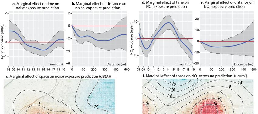
Atmosphere 2020, 11, 422 2 of 21
Atmosphere 2020, 11, x FOR PEER REVIEW 2 of 22
this study), the WHO advises not exceeding a mean value of 200 µg/m3 in an hour, as exposure above
not exceeding a mean value of 200 µg/m3 in an hour, as exposure above this level causes significant
this level causes
inflammation significant
of airways [7]. inflammation of airways [7].
1.1. Cyclists’ Exposure and Transport Justice
1.1. Cyclists’ Exposure and Transport Justice
Cyclists are particularly exposed to these pollutions. Indeed, they do not have a cabin or an
Cyclists are particularly exposed to these pollutions. Indeed, they do not have a cabin or an air
air conditioning system to protect them. A considerable body of literature has compared the levels
conditioning system to protect them. A considerable body of literature has compared the levels of
of exposure to air pollution according to the mode of transportation. Studies have concluded that
exposure to air pollution according to the mode of transportation. Studies have concluded that the
the differences
differences in terms
in terms of exposure
of exposure are inconsistent
are inconsistent [8]. However,
[8]. However, when thewhen the ventilation
ventilation rate is taken rateinto
is
taken into
account, it isaccount,
clear thatit is clear inhale
cyclists that cyclists inhale
more air more air
pollutants pollutants
than other road than other
users. In aroad users.
recent In a
literature
recent literature review, Cepeda et al. [9] have found that car users inhaled an
review, Cepeda et al. [9] have found that car users inhaled an average of only 16% of the total dose inhaled average of only 16%
of the total dose inhaled by cyclists for similar trips. Less information is available
by cyclists for similar trips. Less information is available for exposure to noise, but Okokon et al. [10] for exposure to
noise,found
have but Okokon
that, onet al. [10] cyclists
average, have found that, on to
are exposed average,
6 more cyclists are exposed
dB(A) than car usersto in6Helsinki
more dB(A) than
(Finland),
car users in Helsinki (Finland), and 4.0 in Thessaloniki (Greece), on average
and 4.0 in Thessaloniki (Greece), on average for similar trips, and Apparicio et al. [11] have found for similar trips, anda
Apparicio et al. [11] have found a difference
difference of 1.92 (LAeq,1min) in Montreal (Canada). of 1.92 (L Aeq,1min ) in Montreal (Canada).
Thesecond
The secondmain maincausecauseofofcyclists’
cyclists’ overexposure
overexposure is their
is their direct
direct proximity
proximity to atomajor
a major source
source ofand
of air air
and noise pollution, i.e., road traffic. This proximity is reinforced by planning
noise pollution, i.e., road traffic. This proximity is reinforced by planning policies encouraging road policies encouraging
road sharing.
sharing. In Paris,In this
Paris,
is this is striking
striking when onewhen one observes
observes the development
the development of the network
of the bicycle bicycle network [12].
[12]. In 2001,
In 2001,
the the city permitted
city permitted cyclists tocyclists
use bustolanes
use bus
andlanes andmany
in 2010, in 2010, many streets
one-way one-way streets
were weretoopened
opened cycliststo in
cyclists
both in both(Figure
directions directions (Figure
1). These two1).breaks
Theserepresent
two breaksmajor represent major
increases increases
in available in available
cycling cycling
infrastructures,
but this raises the
infrastructures, butquestion
this raises of the
the quality
question ofof
these infrastructures
the quality of these and the closeness
infrastructures andto the
traffic that they
closeness to
entail.
traffic that they entail.
Figure1.1.The
Figure Thedevelopment
development of
of aa cycling network in
cycling network in Paris
Paris between
between1995
1995and
and2017.
2017.
Cyclists’overexposure
Cyclists’ overexposure supports
supports thethe statements
statements of Gössling
of Gössling [13]transportation
[13] on on transportation
justice.justice. The
The bicycle
bicycle
is is a durable
a durable mode mode of transport
of transport and helps
and helps to reduce
to reduce congestion,
congestion, environmental
environmental noise,
noise, emission
emission of
of greenhouse gas, and health costs. Yet only a minor portion of the space dedicated
greenhouse gas, and health costs. Yet only a minor portion of the space dedicated to transport is used for to transport is
used forinfrastructure,
cycling cycling infrastructure,
and cyclistsandarecyclists are overexposed
overexposed to urban nuisances.
to urban nuisances.
Unfortunately,the
Unfortunately, theproblem
problemofofcyclists’
cyclists’exposure
exposureisisrarely
rarelyconsidered
consideredininthe thecurrent
currentplanning
planning of
of cycling infrastructure. The London Quietways, which provide cyclists with routes
cycling infrastructure. The London Quietways, which provide cyclists with routes that are quiet and far that are quiet
and far
from from[14],
traffic traffic [14], constitute
constitute an inspiring
an inspiring exampleexample which deserves
which deserves special special
mention.mention.
Yet, new Yet, new
studies
studies that
suggest suggest thatinduced
the risk the risk by
induced by air pollution
air pollution could be highercould than
be higher
that ofthan
roadthat of roadAs
accidents. accidents. As
an example,
Künzli et al. [15], using cohort data, have attributed twice the number of deaths to air pollutionair
an example, Künzli et al. [15], using cohort data, have attributed twice the number of deaths to in
pollution into
comparison comparison to road
road accidents accidents
in Europe. in Europe.
More Moreinspecifically,
specifically, in Paris,
Paris, Praznoczy [16]Praznoczy
has found[16]thathas
the
foundassociated
risks that the risks
withassociated
exposure to with
air exposure
pollution toareairconsiderably
pollution arehigher
considerably higher
than those fromthan
roadthose from
accidents.
road accidents.
Nonetheless, theyNonetheless,
conclude thatthey conclude
all these risks that
remainall these risks
small in remain small
comparison with in
thecomparison with
health benefits ofthe
the
health benefits of the physical activity of bicycling, and this is supported by Cepeda et al. [9] and De
Hartog et al. [17]. Unfortunately, to our knowledge, this type of study does not consider exposure to
noise. The current situation is summarized in Figure 2.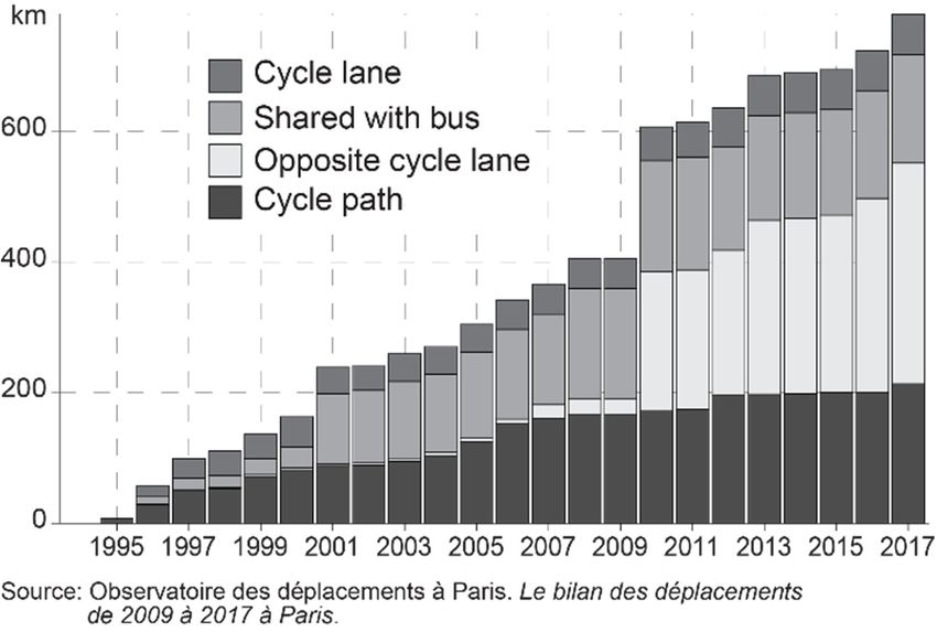
Atmosphere 2020, 11, x FOR PEER REVIEW 3 of 22
physical activity of bicycling, and this is supported by Cepeda et al. [9] and De Hartog et al. [17].
Atmosphere 2020, 11, 422 3 of 21
Unfortunately, to our knowledge, this type of study does not consider exposure to noise. The current
situation is summarized in Figure 2.
Figure 2. The
Figure2. The situation of bicycles
situation of bicycles in
in cities.
cities.
Cities are potentially characterized by high levels of exposure to air and noise pollution which,
Cities are potentially characterized by high levels of exposure to air and noise pollution which,
combined with the current bicycle renaissance and the lack of cycling infrastructure, lead to a situation
combined with the current bicycle renaissance and the lack of cycling infrastructure, lead to a situation
where cyclists
where cyclists are
are overexposed.
overexposed. When When considering
considering thethe collective
collective benefits
benefits of
of urban
urban cycling
cycling (a
(a durable
durable
mode of transportation, and a reduction in health costs and congestion), this
mode of transportation, and a reduction in health costs and congestion), this reveals an injustice reveals an injusticein
in transport.
transport. The combination
The combination of thisof this injustice,
injustice, the renaissance,
the cycling cycling renaissance, and the requirement
and the requirement for
for sustainable
sustainable transportation
transportation in our societyintoday
our society
suggeststoday suggests
a need a need
to rethink ourtopractices
rethink our practices
in cycling in cycling
infrastructure
infrastructure
planning. planning.
Thisnecessitates
This necessitates including
including the
the question
question of of cyclists’
cyclists’ exposure
exposure to to air
air and
and noise
noise pollution
pollution in
inplanning
planning
and working
and working to to understand
understand howhow we we can
can reduce
reduce these
these exposures.
exposures. ManyMany studies
studies have
have already
already tried
tried to
to
identify the factors contributing to cyclists’ exposure to air or noise pollution [18–20],
identify the factors contributing to cyclists’ exposure to air or noise pollution [18–20], but there are but there are
significantlimitations
significant limitationstototheir
theirscope
scope and
and generalization
generalization potential:
potential: fewfew consider
consider noise;
noise; the amount
the amount of
of data
data
is is limited;
limited; there needs
there needs to be replication
to be replication on specific
on specific axes; thereaxes; there
is no is no unbundling
unbundling of background
of background pollution;
pollution;methods
statistical statistical methods
omit omit pseudo-replication,
pseudo-replication, etc. etc.
1.2. The
1.2. TheDevelopment
DevelopmentofofLow-Cost
Low-CostSensors:
Sensors:New
New Paradigm
Paradigm and
and Opportunities
Opportunities
Duringthe
During thelast
lastdecade,
decade,the thedevelopment
developmentofofnew newtechnologies
technologies andand low-cost
low-cost sensors
sensors to to measure
measure air
air and noise pollution has presented opportunities to study these pollutants.
and noise pollution has presented opportunities to study these pollutants. The low-cost sensors The low-cost sensors(in
(in contrast
contrast withwith traditional
traditional monitoring
monitoring network)
network) havedrawn
have drawnattention
attentionfromfrom research
research and institutional
institutional
fields, and
fields, and in
in 2013,
2013, the
the EPA proposed a classification with five five tiers
tiers of
of sensors
sensors to toevaluate
evaluatetheirtheirpotential
potential
use and
use and reliability
reliability [21].
[21]. The
The first
first and second tiers are the most most limited
limited sensors,
sensors, mainly
mainly builtbuilt for
for citizen
citizen
useand
use andcommunity
communitygroups groupsforfor personal
personal andand education
education purposes.
purposes. TheThethirdthird
and and
fourthfourth
tiers tiers
groupgroupmore
accurate devices
more accurate used used
devices to provide
to provide complementary
complementary data (with
data (withhigher
higherspace-time
space-timeresolution)
resolution) to the the
traditional
traditionalmonitoring
monitoringnetworks
networksatata alower
lowercost. Finally,
cost. Finally,thethe
fifth-tier group
fifth-tier group reference
reference sensors thatthat
sensors areare
the
most reliable
the most and and
reliable sophisticated
sophisticatedbut less accessible.
but less The The
accessible. frontiers between
frontiers these
between categories
these categoriesare fuzzy, but
are fuzzy,
the
butlow-cost designation
the low-cost applies
designation to theto
applies first
thethree tiers. Snyder
first three et al. [22]
tiers. Snyder see[22]
et al. in this
see indevelopment
this developmentthe rise
of a new paradigm in the measure of atmospheric pollution (this holds true for
the rise of a new paradigm in the measure of atmospheric pollution (this holds true for noise pollution) noise pollution) and
distinguish four four
and distinguish potential uses uses
potential for these low-cost
for these low-costsensors:
sensors:(1) (1)
supplementing
supplementing routine
routineambient
ambient air
monitoring networks, (2) expanding the conversation with communities,
air monitoring networks, (2) expanding the conversation with communities, (3) enhancing source (3) enhancing source
compliance
compliance monitoring,
monitoring, and and (4) monitoring personal
(4) monitoring personal exposure.
exposure. Morawska
Morawska etet al. [23] realized
al. [23] realized aa
comprehensive review of scientific and grey literature using these low-cost sensors.
comprehensive review of scientific and grey literature using these low-cost sensors. They concluded They concluded that
manufacturers
that manufacturers do not do evaluate
not evaluate these sensors’
these sensors’reliability
reliabilityandand accuracy
accuracy withwithenough
enoughcare. care.AsAsa
a consequence, many research teams started to do this work and some of them report satisfactory
agreement levels with reference sensors when the data are pre- and post-processed. As an example,
the EPA [24] started a program to evaluate 30 sensors without a calibration process. Low-cost sensors
will never replace reference devices, but they offer the opportunity to collect complementary data at
much finer space and time scale because of their affordability, ease of use, and small size [25].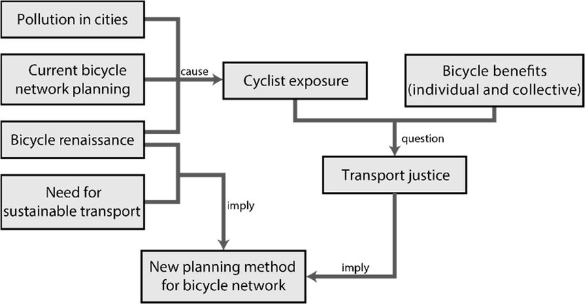
Atmosphere 2020, 11, x FOR PEER REVIEW                                                                          4 of 22

consequence, many research teams started to do this work and some of them report satisfactory
agreement levels with reference sensors when the data are pre- and post-processed. As an example, the
 Atmosphere 2020, 11, 422                                                                                           4 of 21
EPA [24] started a program to evaluate 30 sensors without a calibration process. Low-cost sensors will
never replace reference devices, but they offer the opportunity to collect complementary data at much
finer space   and timeisscale
      This evolution             because
                            a driving      of their
                                        force  in theaffordability,
                                                      research fieldease  of use, and
                                                                      on cyclists’    small to
                                                                                   exposure  size
                                                                                                air[25].
                                                                                                    and noise pollution.
     This   evolution    is a driving  force  in  the research field  on cyclists’ exposure
 Thus, new tools have been made accessible to researchers to address new research goals      to air and noise  pollution.
                                                                                                         like estimating
Thus,  new tools
 the difference   inhave    been for
                      exposure    made    accessible
                                      similar          to researchers
                                                trips according  to thetotransport
                                                                          address new
                                                                                    moderesearch   goals like estimating
                                                                                          [9,26], measuring     the short
the
 term health impact of cyclists’ exposure to air pollution [27], or modelling and measuring
    difference    in  exposure    for similar   trips according   to the transport   mode  [9,26],  predictingthe    short
                                                                                                                 cyclists’
term health impact of cyclists’ exposure to air pollution [27], or modelling and predicting cyclists’
 exposure in urban environments [18–20,28,29].
exposure in urban environments [18–20,28,29].
      Our study continues this research trend and investigates more specifically the case of Paris
     Our study continues this research trend and investigates more specifically the case of Paris (France).
 (France). In September 2017, data were collected on cyclists’ exposure to noise and nitrogen dioxide
In September 2017, data were collected on cyclists’ exposure to noise and nitrogen dioxide (NO2) by using
 (NO2 ) by using low-cost sensors. The main goal of the paper is to develop a methodology based on
low-cost sensors. The main goal of the paper is to develop a methodology based on an extensive mobile
 an extensive mobile data collection using low-cost sensors to determine which factors of the urban
data collection using low-cost sensors to determine which factors of the urban micro-scale environment
 micro-scale environment contribute to reduce cyclists’ multi-exposure and to what extent.
contribute to reduce cyclists’ multi-exposure and to what extent.
2. Conceptual Framework for Modelling Cyclists’ Multi-Exposure
2. Conceptual Framework for Modelling Cyclists’ Multi-Exposure
     To answer this research question, we propose the conceptual framework illustrated in Figure 3.
     To answer this research question, we propose the conceptual framework illustrated in Figure 3.

                                           Figure 3. Conceptual framework.
                                           Figure 3. Conceptual framework.
       Cyclists are simultaneously exposed to noise and air pollution, measured here as the concentration
      Cyclists are3 ) simultaneously    exposed to noise and air pollution, measured here as the concentration
 of NO2 (µg/m          and noise level (dB(A)). These two exposures depend on the characteristics of the
of NO2 (µg/m ) and noise level (dB(A)). These two exposures depend on the characteristics of the micro-
                3
 micro-scale-environments through which they travel and the background pollution. The latter follows
scale-environments through which they travel and the background pollution. The latter follows temporal
 temporal and spatial patterns. Weather has a direct impact on noise propagation and on NO2 chemical
and spatial patterns. Weather has a direct impact on noise propagation and on NO2 chemical interactions
 interactions and dispersion. Finally, the sensors used have a systematic variability in their measurement
and dispersion. Finally, the sensors used have a systematic variability in their measurement that has to
 that has to be controlled. Micro-scale-environment depicts a distinction of the more classical concept of
be controlled. Micro-scale-environment depicts a distinction of the more classical concept of micro-
 micro-environment
environment              in exposure
                in exposure    studies.studies.    It describes
                                         It describes            “an individual
                                                         “an individual   volumevolume      or an aggregate
                                                                                    or an aggregate           of locations,
                                                                                                     of locations, or even
 or even   activities   within  a location   [ . . .  ] hav[ing]  an  homogeneous       concentration
activities within a location […] hav[ing] an homogeneous concentration of the pollutant being evaluated” of the pollutant
 beingsuch
[30],    evaluated”
             as home,[30],   such as home,
                         workplace,   in-publicworkplace,
                                                     transport,in-public  transport,
                                                                 cycling etc.  As we cycling    etc. As
                                                                                        need a more      we need a more
                                                                                                      disaggregated    and
 disaggregated    and    geographical    perspective,     we  define  in this study   the micro-scale-environment
geographical perspective, we define in this study the micro-scale-environment as a chunk of space and                  as a
 chunk    of space  and   time  with a  homogeneous
time with a homogeneous concentration of pollutants.        concentration    of pollutants.
       Somestudies
      Some    studies have
                        have already
                              already investigated
                                       investigated the  the characteristics
                                                              characteristics of
                                                                               of the
                                                                                  the urban
                                                                                       urban environment
                                                                                             environment which
                                                                                                             which might
                                                                                                                     might
 have   an  impact   on  NO    concentration      or   noise level. These   works    are inspired
have an impact on NO2 concentration or noise level. These works are inspired by the classical Land
                             2                                                                     by the  classical Land
                                                                                                                       Use
 Use Regression (LUR), usually applied to data collected by static monitoring stations [31]. The factors
 most often considered are as follows:
       First, road traffic might be measured as real time traffic recorded specifically during the time
 span of the study [32,33], estimations of daily traffic volume [34–36], or the type of roads taken by
 the cyclist [19,28,29]. In all cases, road traffic is associated with cyclists’ greater exposure to air and
 noise pollution.
       Second, vegetation is integrated in studies as the number of trees around the samples [19,36],
 the presence of a park [20,35–37], or its density [34]. The results remain inconsistent and the role of
Atmosphere 2020, 11, 422 5 of 21
vegetation in the absorption and deposit of air and noise pollution seems to be small in comparison
with the “park effect” induced by the increased distance from pollution sources. In some cases, the
vegetation could even retain and trap air pollution (notably in urban canyons) preventing its vertical
dispersion [38].
Third, land use, i.e., the density of residential, industrial, and commercial areas, open spaces, and
the diversity of land use are indicators generally associated with higher or lower concentration of noise
and air pollution. Indeed, neighborhoods with a higher concentration of activities and population
accumulate many pollution sources [33,35,36] and, thus, higher levels of pollution are more likely to be
observed there.
Fourth, urban morphology, i.e., the build density, street canyons, wind permeability, or the density
of intersections are factors describing the geometry of the city and might play an important role in air
pollution trapping (canyon effect) and noise propagation [39–41].
3. Material and Methods
3.1. Case Study
Paris is an interesting case study for many reasons. First of all, the city has experienced a typical
evolution of bicycle use since the 20th century. The bicycle had fallen into disuse at the end of the
Second World War and was largely replaced by the car due to the latter becoming more widely available
and the disappearance of cycling sidewalks [42]. The bicycle lost its status as a means of transport and
was confined to sports and leisure uses. It was only in the 1980s that the bicycle made its comeback
in cities as a means of transportation, promoted by the ecological movement and the rising cost of
other means of transport. Some authors name this new period the “bicycle renaissance” [43]. In Paris,
one can note a new increase in bicycle use at the beginning of the 2000s, after a period of stagnation
since 1970. Between 2001 and 2010, the number of daily trips made by bicycle doubled and reached
650,000 trips in central districts (within the city) [44].
Second, Paris is a city with relatively high levels of air and noise pollution. AirParif and BruitParif
are two associations charged by the French government with monitoring air and noise pollution,
respectively, in the region of Île de France. In its 2017 annual report, AirParif indicates that, over 6 days,
the O3 and particulate matter concentrations exceeded the fixed threshold (for a total of 12 days).
The association estimates that 1.3 million residents in the region are exposed to NO2 concentration
levels higher than the standard for annual exposure and that 10 million are living in places where
the French quality standard for annual exposure to PM2.5 (10 µg/m3 ) is exceeded. The proximity to
road traffic appears to be the main source of pollution in the report [45]. The maps of annual NO2
concentrations (available in the document [45]) depict a clear gradient from central to outlying areas.
This phenomenon is explained by the higher density of activities, population, trips, and equipment
and a more densely built environment, less favorable to air pollution dispersion.
In 2017, BruitParif [46] estimated that only 15% of the region’s population living in dense urban
areas was exposed to annual daily mean levels of noise below 53 dB(A) (the WHO guideline) and
11% was exposed to levels higher than 68 dB(A) (the intervention threshold defined by the European
Union). Overall, 65,607 years of healthy life expectancy are lost annually in the region because of noise
exposure. Again, maps are available in the report [46] and transport (air, rail, and road transport)
appears to be the main source of this problem.
Therefore, in this context where the number of cyclists is increasing and the levels of exposure to
air and noise pollution are potentially high, a study on cyclists’ multi-exposure is clearly justified.
3.2. Primary Data Collection and Structuration
Primary data was collected in Paris over four days in September 2017 (4 September to 7 September).
Three participants (two graduate students and one professor) cycled approximately 100 km everyAtmosphere 2020, 11, 422 6 of 21
day between 08:00 a.m. and 6 p.m. This study has been approved by the Institutional Review Board
(Ethical Review Board of Institut national de la recherche scientifique) (Project No CER-15-391).
We realized a mobile data collection using portable low-cost sensors to measure the exposure
on three participants. This research falls within the new paradigm of data collection on individual
exposure. Indeed, classical monitoring networks have been found to be not very representative of
individual exposure [47,48]. This can be explained by the low density of their spatial coverage that
fails to measure the micro-variations of pollution in urban areas [49–51]. Moreover, these stations
are generally not located directly on streets, but some meters above the ground or on the top of
buildings, which contributes to an underestimation of people’s direct exposure at road level [47,52,53].
MacNaughton et al. [34] reports values for NO2 (ppb) of 24.2 ppb measured by mobile sensors (sampled
concentration) versus 15.9 ppb by static stations (background pollution) on a designated bike lane.
Different authors likewise observed higher variations for other pollutants [20,54,55].
The use of low-cost sensors and a mobile approach has several drawbacks. First, because of its
ephemeral nature, the mobile data collection is not suited for an assessment of seasonal variations
of pollution. This could be achieved by repeated and periodic data collection but with a significant
increase of the costs. This type of question must preferably be investigated with data collected from
traditional monitoring networks. Second, this approach produces less reliable measurements and
might not provide an accurate estimation of typical values of pollution concentrations on specific streets.
To overcome these limitations, Van den Bossche et al. [47] and Hatzopoulou et al. [56] propose an
intensive approach based on repetitive sampling of the same segments. The repetition of measurement
is a way to compensate for the considerable variability of the data and the lower accuracy of the
sensors. However, this method limits the spatial coverage of the study area and, thus, the diversity of
sampled environments, which is one of the main appeals of the use of low-cost sensors combined with
mobile data collection. Therefore, we propose an extensive approach (in opposition to an intensive
approach), aiming to maximize the spatial coverage and the diversity of environments travelled. The
goal is not to estimate precisely the expected values of exposure to pollution on a specific segment
(which is difficult with low-cost sensors), but rather to understand the impacts of urban environmental
characteristics in their (almost) full range of values on individual exposure. A similar approach has
already been applied successfully in Ho Chi Minh City (Vietnam) [57], Portland (Oregon, USA) [35],
Ghent (Belgium) [40], Flanders (Belgium) [58] (even if the expression “extensive data collection” was
not used). The replicability of the study is not affected by this design. Indeed, the trips are recorded and
could be replicated. Obviously, the exact conditions of traffic and meteorology cannot be reproduced,
but this is also true for the intensive design.
The trips were defined before the data collection with GoogleMaps and stored with MyMaps.
During the data collection, the participants had to follow the routes on their smart phone fixed on the
handlebar and to modify them in case of perturbation (closed street, road work, stairs, etc.). Following
the extensive design approach, the trips were chosen to maximize the spatial coverage and the diversity
of urban environments, and to reduce repetitive samples on the same segments.
To measure the nitrogen dioxide (NO2 ) concentration (µg/m3 ), temperature (◦ C), and humidity (%),
participants were equipped with an Aeroqual Series 500 Portable Air Quality monitor (Aeroqual Limited,
Auckland, New Zealand) and its two sensors (one for NO2 concentration and one for temperature
and humidity). This device has a temporal resolution of 1 min. According to the Aeroqual supplier’s
product information, the NO2 sensor has the following characteristics: range (0–1 ppm), minimum
detection (0.005 ppm), accuracy of factory calibration (Atmosphere 2020, 11, 422 7 of 21
strong linear relationship with reference analyzer [60]. No O3 sensor was available during this data
collection, but we propose another approach based on statistical methods to control its contribution to
the measurements (see Sections 3.3 and 5.1). Aeroqual Series 500 monitors have largely been used in
numerous studies on individual exposure or air pollution mapping, e.g., [11,19,61–63].
To measure noise level (LAeq, 1min , dB(A)), a Brüel and Kjaer Personal Noise Dose Meter (Type 4448,
class 2, conform to IEC 61252:2002 and ANSI S1.25:1991 standards) was fixed on the participant’s left
shoulder (as recommended by the manufacturer) facing the road with their wind-shield. This device
has a temporal resolution of 1 min and has the following characteristics: exchange rate (3 dB), sound
level range (certified 65–140 dB, reliable down to 58 dB), accuracy (±2 dB). This device does not record
the frequency spectra. As recommended by the manufacturer, the Personal Noise Dose Meters were
calibrated once a day using the Sound Calibrator Type 4231 (calibration accuracy ±0.2 dB). Triathlon
GPS watches (Garmin 910 XT) were used to record the GPS track of the trips with a temporal resolution
of 1 s. Finally, action cameras (Garmin Virb XE) fixed to the handlebar were used to record videos of
the trips.
More recent sensors of noise and air pollution however offer a lower temporal resolution, but
at higher variability cost in the collected data. A temporal resolution of 1 min is sufficiently detailed
considering that with a mean speed of 15 km/h, a cyclist can ride only 250 m.
The GPS tracks were map-matched to the Open Street Map (OSM) road network using the
algorithm OSRM [64]. This data structuration step was validated manually by using videos of the trips.
The traces were cut as 1-min segments (temporal resolution of the sensors) and all the measurements
were assigned to these segments by using timestamp (the clocks of each device were synchronized
every morning during the data collection). The OSM street network dataset was selected rather than
the official city network because, the OSM network nomenclature is common to each city in the world
and thus will allow easier comparisons between papers using this dataset in this field study [57].
Only 5% of the sampled segments were not categorized or not present in the database and were thus
classified as “unclassified roads”. Apart from missing data, OSM is criticized for inaccuracy in the road
typology, notably for roads smaller than primary roads [65]. According to the same work, the quality
of the OSM data increases with the density of contributors, and they are numerous in big cities like
Paris. A more recent study concludes that “the Paris OSM road network has both a high completeness
and spatial accuracy [ . . . ] and is found to be suitable for applications requiring spatial accuracy up to
5–6 m.” [66]. This level of accuracy is appropriate for our study. The data was not pre-processed before
data analysis. Only the observations with missing values or measurements exceeding the measurement
ranges were removed.
3.3. Data Analysis—Building a Model to Estimate the Impact of Micro-Scale Environment
Let us recall here that the main goal of this study is to identify the factors of the micro-scale-
environment that contribute to cyclists’ multi-exposure and to evaluate the extent of these contributions.
The most used method to achieve this goal is regression analysis, with the exposure measurements as
dependent variables. However, the use of low-cost sensors combined with the mobile extensive data
collection design raises many methodological challenges in the analysis of the data.
First, we must deal with the problem of pseudo-replication. Indeed, two factors violate the
condition of independence of observations: the day of data collection and the sensor. Day to day,
because of specific weather and/or traffic conditions, exposure values might vary systematically (part of
background pollution). In the same manner, two observations coming from the same sensor are more
likely to be similar than two observations coming from different sensors (sensor effect). Hence, the
day of data collection and the sensors are incorporated in the models as random effects because they
impose a hierarchical structure on the dataset (grouping effect), and thus allows us filter out these
effects from the data.
Still with regard to pseudo-replication, the temporal autocorrelation has to be controlled. Our
data can be seen as a temporal series, so two consecutive observations are more likely to be similarAtmosphere 2020, 11, 422 8 of 21
than two observations selected randomly. This is rarely done in this field study, but it is necessary to
obtain unbiased coefficients in the model.
Secondly, the cyclists’ exposure measurement combines both the background pollution
(structural spatial-temporal variations) and the immediate pollution specific to the micro-scale
environment (which is the primary interest in this study). Thus, to estimate the role of the micro-scale
environment, it is essential to distinguish them. To do so, some studies propose using external data
coming from static stations to adjust the exposure data by subtracting the background pollution [40],
or by adding it as a covariate [20,34] in the analysis. Considering the fact that temporal and spatial
patterns of background pollution are integral parts of the collected data, we propose instead to model
them directly as nonlinear terms [67]. These terms make it possible to capture the systematic variation
through space and time of our exposure data and to model the effects of the micro-scale environment,
without using Supplementary Data. This method has already been proven to be useful in modelling
cyclists’ exposure to noise [57]. Nonlinear terms (e.g., splines) are regularly employed to model
exposure to air pollution [40,41]. For space, a bivariate spline can be constructed from the coordinates
of the sampling segments. In the model, it reflects the systematic spatial variation of noise and NO2 ,
everything else being equal. Thus, it can be interpreted as the spatial pattern of the background
pollution. In the same way, a univariate spline for time can be built from the timestamp of the sampling
segment and can be interpreted as the temporal pattern of the background pollution.
Finally, we have to model two dependent variables simultaneously: noise and NO2 exposures.
Considering the fact these two pollutions share some of their sources, it is likely that they share some
variance. Thus, we propose to model them simultaneously with a multivariate regression model [68].
Theoretically, this permits us to be closer to the multi-exposure concept. Statistically this model allows
to consider a potential correlation between the two dependent variables. The proposed model is
detailed bellow:
yz ∼ D(µz , σz ) (1)
l
X n
X k
X
µz[i] = αz + Xz[i] ∗ βzl[i] + αzsens[ij] + αzday[id] + fzp X[i] + ∅p εzi−p + εz
p=1 p=1 p=1
αz capt ∼ normal 0, σz capt
αz jour ∼ normal 0, σz jour
X
εz ∼ normal 0, ε
with i an observation (1-min segment),
D a specific distribution (Gaussian or student in this article),
z a dependent variable (NO2 concentration or noise level in this article),
α the general intercept,
l the number of fixed linear parameters in the model,
j a sensor and d a day of the week,
α_sens a vector of intercepts for each sensor, normally distributed and centered on 0,
α_day a vector of intercepts for each day, normally distributed and centered on 0,
n the number of nonlinear parameters in the model,
f a nonlinear function,
k the maximal lag to consider for the temporal autocorrelation parameter (MA),
The noise vector εi for each observation i is jointly normal (and centered on 0), so that the outcomes
for a given observation are correlated. The variances of dependent variables are assumed to be constant.
The model above is implemented in a Bayesian framework in R [69] with the package brms [70]
based on STAN [71]. The used priors are described in Supplementary Material (S1). We fitted theAtmosphere 2020, 11, 422 9 of 21
model using four chains, each with 10,000 iterations where the first 1000 were used as a warmup for
sampling realized with a No-U-Turn Sampler (NUTS).
The predictors are described in Table 1. Following the literature review presented above, many
terms describing the 1-min segment characteristics (slope, speed of the cyclists, and number of
intersections encountered), the road traffic (type of road, type of cycling infrastructure, low-speed
zone, and distance to the closest main road), land use (activity density in a 50 m buffer), and vegetation
(canopy density in a 50 m buffer) were introduced as independent variables. Two predictors describing
the urban form were also used: the percentage of visible sky from the ground (street canyon proxy),
the fetch index (indicator of potential local wind exposure), and its interaction with wind. Finally, two
covariates describing the weather conditions were added to the model: the temperature (measured by
the portable air pollution sensors) and the wind speed (available for each hour from Paris weather
stations). Humidity was discarded because of its strong correlation with temperature. Details of the
calculations and the data source of each index are available in Supplementary Material (S2).
Table 1. Independent variables included in the regression model.
Dimension Variable Type
Slope (%) Linear effect
Cyclist’s speed (km/h) Linear effect
Number of intersections encountered Linear effect
Type of road (proportion of 1 min) Linear effect
Low-speed zone 30 (0–1) Linear effect
Distance from main road when on cycling infrastructure (m) Nonlinear effect
Micro-environment Industrial activity land use density (%) in a 50 m buffer Linear effect
Vegetation density (%) in a 50 m buffer Linear effect
Sky view factor index (%) Linear effect
Fetch index (%) Linear effect
Fetch index * wind speed Linear effect
Temperature (◦ C) Linear effect
Wind speed (km/h) Linear effect
Background- Coordinates (X,Y) Nonlinear effect
pollution Number of minutes since 07:00 AM Nonlinear effect
Day of the data collection Random intercept
Control factors Sensor Random intercept
Temporal autocorrelation MA2 term
4. Results
4.1. Descriptive Analysis
Before presenting the results of the analysis, some descriptive statistics should be reported. A
total of 3822 observations of 1-min segments were collected for a total of 64 h and 964 km traveled.
Figure 4 is a map of the trips accomplished. This represents an extensive coverage, we calculated that
if we divide the intra-muros area of Paris in squares of 250 m length, then we have sampled, at least
once, 52% of them.
Table 2 displays descriptive statistics of NO2 and noise exposure, however, these values must be
interpreted with caution. They are raw data coming from low-cost sensors and could overestimate
real exposure, especially for NO2 because of cross sensitivity of the sensor to O3 (see Section 3.2)
and the strong day to day variation. Indeed, we observed a difference of 35 µg/m3 between higher
(4 September) and lower (3 September) days for NO2 mean exposure. For time of day, over the
same period, the NO2 concentration recorded by AirParif had a mean of 37.8 µg/m3 with 10% of the
records below 10 µg/m3 and 90% of the records higher than 77 µg/m3 . A direct comparison of these
values is hazardous considering that the locations of the AirParif fixed stations are chosen to reflect
regional air concentration, while mobile individual exposure is measured directly in streets. AlthoughAtmosphere 2020, 11, 422 10 of 21
Atmosphere 2020, 11, x FOR PEER REVIEW 10 of 22
various studies found considerable gaps between regional concentrations and individual exposure
a map during
obtained of the trips accomplished.
a mobile This represents
data collection an it
[20,34,35,72], extensive coverage,
is still likely wesensors
that our calculated that if we the
overestimate divide
the intra-muros
cyclists’ exposure. area of Paris in squares of 250 m length, then we have sampled, at least once, 52% of
them.
Figure 4. Study
Figure areaarea
4. Study andand
sample routes.
sample routes.
NO2 is characterized by a stronger temporal autocorrelation than noise, meaning that consecutive
Table 2 displays descriptive statistics of NO2 and noise exposure, however, these values must be
values of NO2 concentration are more similar than values of noise level. This is explained by the
interpreted with caution. They are raw data coming from low-cost sensors and could overestimate real
fact that noise
exposure, is more impacted
especially for NO2 because by short oftime
crossevents like aoftruck
sensitivity passing,
the sensor to honking, or the 3.2)
O3 (see Section crossing
and the
of strong
a residential street. NO
day to day variation. 2 is less influenced by these events because of its slower dispersion
Indeed, we observed a difference of 35 µg/m3 between higher (4 September) and its
accumulation
and lower (3inSeptember)
air. In contrast,
days for the NOspatial autocorrelation is stronger for noise, meaning that noise
2 mean exposure. For time of day, over the same period, the NO2
exposure is morerecorded
concentration characterized by spatial
by AirParif had structures
a mean of than NO2 .3 with 10% of the records below 10 µg/m3
37.8 µg/m
Not surprisingly, the correlation between
and 90% of the records higher than 77 µg/m . A2 direct comparison NO
3 concentration and of noise level
these (at the
values 1-min
is hazardous
resolution
consideringlevel)
thatisthe
weak (Pearson:
locations 0.11) and
of the AirParif thisstations
fixed corroborates
are chosenprevious studies
to reflect for air
regional theconcentration,
same air
pollutant [19] or PM [73]. Davies et al. [74] have reported a moderate
while mobile individual exposure is measured directly in streets. Although various studies found
2.5 correlation (0.5) of exposure to
NO and noise
considerable
2 but their data were collected in less diversified environments
gaps between regional concentrations and individual exposure obtained during a mobile and aggregated in 5-min
observations (compared
data collection to 1 min
[20,34,35,72], it isinstill
ourlikely
study).
thatDekoninck
our sensorsetoverestimate
al. [40] suggestthe in their analysis
cyclists’ exposure. that air
pollutionNOcorrelates with noise
2 is characterized by when considering
a stronger temporalonly low frequency
autocorrelation thannoise (caused
noise, by engine).
meaning This
that consecutive
implies
valuestoofdiscard all the higher
NO2 concentration arefrequency
more similar noise produced
than values of bynoise
honks, breaks,
level. and
This is other events
explained by theinfact
thethat
urban
noiseenvironment
is more impacted to which the cyclists
by short are also
time events likeexposed. In our honking,
a truck passing, case, the correlation between
or the crossing noise
of a residential
andstreet.
NO2NO 2 is less
could alsoinfluenced
be reducedby bythese events becauseerror
the measurement of itsofslower dispersion and its accumulation in air.
NO2 sensors.
In Table
contrast,
3 showsthe the
spatial
totalautocorrelation
time spent on each is stronger
type of road for during
noise, the
meaning that noiseThis
data collection. exposure is more
information
characterized
comes from the OSM by spatial
roadstructures
network (key NO2.
thanHighway), and a formal description of each type is available
online inNot surprisingly,
the OSM documentationthe correlation [76]. between NO2 concentration and noise level (at the 1-min resolution
level) is weak (Pearson: 0.11) and this corroborates previous studies for the same air pollutant [19] orAtmosphere 2020, 11, 422 11 of 21
Table 2. Descriptive statistics for dependent variables.
Statistic NO2 (µg/m3 ) LAeq, 1 min (dB(A))
Mean a 163.1 72.4
Standard deviation a 37.2 4.5
Percentiles
5 107.2 65.0
10 118.8 66.5
25 137.2 69.1
50 161.4 71.6
75 185.4 74.0
90 209.5 76.0
95 225.6 77.3
99 76.5 78.9
ACF with
K=1 0.70 0.61
K=2 0.54 0.36
Moran I 0.18 (d = 300) 0.31 (d = 200)
Note: to calculate Moran’s I statistic, we used a binary matrix and defined as neighbors of the segment i all the
segments in a buffer of length d around i with d ranging from 50 to 500 m with a step of 50 m. Only the highest
values are here reported. a Mean and SD of dB values are computed using the seewave package [75]. These values
are raw data and must be interpreted with care, especially the NO2 values which probably overestimate the real
individual exposure.
Table 3. Time spent on each type of road and cycling infrastructure.
Total Time
Minutes %
Road type
Primary road 873 22.8
Secondary road 697 18.2
Tertiary road 377 9.9
Residential street 569 14.9
Pedestrian path 105 2.7
Service 208 5.4
Cycleway 802 21.0
Unclassified 191 5.0
On street cycling infrastructure
Bicycle lane 224 5.9
Opposite lane 106 2.8
Shared bus lane 325 8.5
4.2. Model Adjustment
To build the multivariate regression model, we started with two models in which NO2 and noise
exposures were modelled as bivariate Gaussian distribution and bivariate student distribution to
model formally the correlation between residuals. However, we observed that NO2 and noise did
not follow the same type of distribution. A Gaussian distribution was more suited for noise and a
student distribution for NO2 to approximate their respective original distributions. With two different
distributions, it is no longer possible to model formally the residual correlation between the two
variables, but the latter was weak in the previous models (0.05 for the bivariate student model and
0.04 for the bivariate Gaussian model). Therefore, we decided to keep the model with two different
distributions. The graphical posterior predictive checks, which assess the quality adjustment between
the original data and the predictions of the model, are available in the Supplementary Material S4.
They show that the model is well fitted and managed to reproduce the original distribution of the
variables. Note that the values are reported as follows: mean (0.05–0.95 credibility interval).
All models’ parameters converged (Rhat = 1.0) and all the trace plots display important mixing
(four chains with random start values, with 10,000 iterations, posterior distribution plots are available
in Supplementary Material S3). For the NO2 equation, Bayes R2 is 0.31 (0.29–0.33) when keeping onlyAtmosphere 2020, 11, 422 12 of 21
the fixed effects, and 0.54 (0.53–0.56) with the random effects. Respectively, for noise equation, Bayes
R2 are 0.45 (0.43–0.46) and 0.46 (0.44–0.47). Again, the temporal autocorrelation is stronger for NO2
exposure (MA [1] = 0.57 (0.54–0.60)) than noise exposure (MA [1] = 0.48 (0.45–0.51)), but this effect
has been well controlled by the mode because no more spatial or temporal autocorrelations were
remaining in model residuals (dB(A) ACF at lag 1 = −0.00, at lag 2 = 0.01, NO2 ACF at lag 1 = −0.04,
at lag 2 = 0.06).
4.3. Controlling for the Background Pollution
To control the background pollution, we introduced different terms in the model. First, we added
random intercepts varying by day. The noise exposure varied weakly within days of the data collection
(variation lower than 0.5 dB(A), Table 4). For the NO2 concentration, we noted a lower concentration on
Tuesday (on average −29.5 µg/m3 ) and higher concentrations on Thursday (on average +15.8 µg/m3 ).
They represent 18% and 10% of the global average we reported above, respectively. This clearly
indicates that NO2 exposure is more dependent on data collection days rather than noise exposure.
This stresses the necessity to include this effect in the model.
Table 4. Model’s fixed and random effects.
NO2 (µg/m3 ) LAeq (dB(A))
Estimate S.E. 0.05 CI 0.95 CI Estimate S.E. 0.05 CI 0.95 CI
Fixed terms
Intercept 128.65 28.44 72.58 184.56 70.49 2.35 65.83 74.92
Temperature 1.72 0.78 0.22 3.25 0.07 0.09 −0.10 0.25
Wind speed −0.99 0.54 −2.06 0.08 −0.02 0.07 −0.16 0.13
Fetch index −0.07 0.06 −0.18 0.05 0.00 0.01 −0.02 0.02
Sky view factor index −0.06 0.04 −0.15 0.03 0.02 0.01 0.01 0.03
Primary road Ref. Ref.
Secondary road 1.88 1.58 −1.16 5.01 −0.98 0.21 −1.40 −0.56
Tertiary road −1.24 1.92 −5.02 2.52 −1.88 0.27 −2.40 −1.36
Residential street −1.05 1.82 −4.66 2.52 −4.08 0.26 −4.58 −3.57
Pedestrian street −5.68 3.02 −11.57 0.27 −2.72 0.43 −3.57 −1.89
Service road 3.67 2.30 −0.87 8.16 −1.44 0.32 −2.07 −0.80
Cycleway 0.86 1.59 −2.25 3.93 −1.45 0.23 −1.90 −0.99
Unclassified 1.84 2.23 −2.53 6.19 −2.72 0.31 −3.33 −2.10
Cycle lane −0.82 1.98 −4.68 3.04 0.40 0.28 −0.15 0.94
Opposite cycle lane −0.43 2.83 −5.99 5.14 −0.63 0.40 −1.42 0.15
Shared road −5.75 9.67 −24.53 13.14 0.09 1.88 −3.58 3.78
Shared with bus lane 0.97 1.68 −2.30 4.22 0.52 0.23 0.06 0.97
Low-speed zone 30 −1.93 1.39 −4.63 0.78 −0.58 0.20 −0.97 −0.19
Industrial activity land use 0.03 0.03 −0.03 0.09 0.01 0.00 0.00 0.02
Vegetation density 0.14 0.05 0.05 0.23 −0.02 0.01 −0.03 −0.00
Number of intersections 0.20 0.11 −0.02 0.42 0.03 0.02 −0.00 0.06
Segment slope 0.36 0.22 −0.07 0.80 0.04 0.03 −0.03 0.10
Random intercepts
Day of the week
Monday 2.47 14.41 −19.72 24.09 −0.67 0.60 −1.56 0.10
Tuesday −29.50 14.40 −51.63 −7.70 0.27 0.59 −0.55 1.10
Wednesday 11.13 14.40 −10.89 32.92 0.16 0.58 −0.62 1.01
Thursday 15.80 14.44 −6.29 37.71 0.24 0.59 −0.56 1.13
Participant
ID1 11.83 17.89 −14.62 38.32 0.52 1.19 −1.03 2.06
ID2 10.70 17.89 −15.78 37.26 0.19 1.19 −1.35 1.71
ID3 −22.50 17.90 −49.09 4.09 −0.69 1.19 −2.28 0.81
Temporal autocorrelation
MA [1] 0.57 0.02 0.54 0.60 0.48 0.02 0.45 0.51
MA [2] 0.18 0.01 0.15 0.21 0.14 0.02 0.11 0.17
Second, we added nonlinear terms to control hourly systematic variation of noise and air pollution
(Figure 5a,d). We expected these trends to follow road traffic patterns. For both noise and NO2Atmosphere 2020, 11, 422 13 of 21
concentration, the presence of an effect is evident. In both cases, the horizontal line represents the
centered daily mean and allows us to observe when the exposure values are higher and lower during
the day. For NO2 , one can distinguish three main phases. The first between 8 a.m. and 10 a.m. is
characterized by a decreasing level of exposure, followed by an important rise, reaching its peak at
1:30 p.m., and finally a decrease until 7 p.m. The effect size is in the order of 20 µg/m3 between the
period with the higher and the lower concentration levels. The pattern of noise exposure is totally
different. It starts with higher levels of noise at 8 a.m. and then diminishes until 2 p.m. at its lowest
level. A new increase starts at 4 p.m. and seems to end at 7 p.m. These variations follow a typical
road traffic pattern with first rush hours in the morning, and a second one at the end of the afternoon.
Again, the size of the effect is far from negligible, with a difference of almost 2 dB(A) between the
noisiest
Atmosphereand
2020,quietest
11, x FORperiods.
PEER REVIEW 13 of 22
Figure 5. Marginal
Figure Marginal effects ofof model’s
model’s nonlinear
nonlinear terms.
terms. Note:
Note: These mapsmaps show
show thethe splines
splineson onthe
the
geographic coordinates introduced in in the
themodel.
model. They
They do
donot
notrepresent
representaaconcentration
concentrationmap mapfor
forthe
theNO
NO22
or noise. These spatial and temporal trends are valid only for the data collection period; they cannot
trends are valid only for the data collection period; they cannot be be
generalized over the whole year.
year. (a)
(a) Marginal
Marginal effect
effectof
oftime
timeononnoise
noiseexposure
exposureprediction;
prediction;(b) (b)Marginal
Marginal
effect of distance on
on noise
noise exposure
exposure prediction;
prediction;(c)
(c)Marginal
Marginaleffect
effectofofspace
spaceon
onnoise
noiseexposure
exposureprediction
prediction
(dB(A)) (d) Marginal effect
effect of
of time
timeon
onNO exposureprediction;
NO22exposure prediction;(e)
(e)Marginal
Marginaleffect
effectofofdistance
distanceononNONO22
exposure 3).3
exposure prediction;
prediction;(f)
(f)Marginal
Marginaleffect
effectof
ofspace
spaceononNONO22exposure
exposureprediction
prediction(µg/m
(µg/m ).
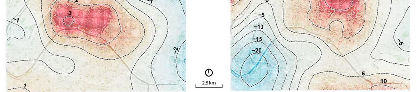
Finally, nonlinear
Second, we added spatial terms
nonlinear termswereto introduced
control hourly to control for the
systematic systematic
variation spatial
of noise andbackground
air pollution
variation of the two pollutions. They are mapped in Figure 5c,f. These
(Figure 5a,d). We expected these trends to follow road traffic patterns. For both noise maps represent the continuous
and NO2
functions (splines)
concentration, the adjusted
presence by of the
an model.
effect isWe thus display
evident. In boththem withthe
cases, a higher resolution
horizontal (100 m) than
line represents the
the sampling
centered dailyresolution
mean andbecause
allows us of to
this continuous
observe when nature. Both effects
the exposure valuesare
aresignificant,
higher and withlowerdifferences
during the
greater
day. Forthan
NO2,5onedB(A) between places
can distinguish with phases.
three main the highest andbetween
The first lowest levels of noise
8 a.m. and 10 a.m. exposure, and a
is characterized
difference of more
by a decreasing levelthan
of exposure, 3
30 µg/m followed
for NO2by exposure.
an importantThe rise,
central areas,its
reaching north
peakofat the
1:30Seine
p.m., River, are
and finally
a decrease until
characterized by7 systematically
p.m. The effecthigher
size is levels
in the order
of noiseof 20 NO23 between
andµg/m exposurethein period
comparisonwith the higher and
to peripheral
the lower
areas. Theconcentration
spatial trendlevels.
of NOThe pattern
2 shares someof noise exposure
similarities withis the
totally different.
annual It starts with higher
NO2 concentration map
levels of noise
proposed at 8 a.m.in
by AirParif and then
2017 diminishes
[45]. For noise,until
the2 resemblance
p.m. at its lowest level.
is less A new increase
pronounced, startson
however, at 4both
p.m.
and seems to end at 7 p.m. These variations follow a typical road traffic pattern with first rush hours in
the morning, and a second one at the end of the afternoon. Again, the size of the effect is far from
negligible, with a difference of almost 2 dB(A) between the noisiest and quietest periods.
Finally, nonlinear spatial terms were introduced to control for the systematic spatial background
variation of the two pollutions. They are mapped in Figures 5c and 5f. These maps represent theYou can also read