Fishermen Follow Fine-Scale Physical Ocean Features for Finance - NVS
←
→
Page content transcription
If your browser does not render page correctly, please read the page content below
ORIGINAL RESEARCH
                                                                                                                                          published: 19 February 2018
                                                                                                                                       doi: 10.3389/fmars.2018.00046

                                             Fishermen Follow Fine-Scale
                                             Physical Ocean Features for Finance
                                             James R. Watson 1,2*, Emma C. Fuller 3 , Frederic S. Castruccio 4 and Jameal F. Samhouri 5
                                             1
                                              College of Earth, Ocean and Atmospheric Sciences, Oregon State University, Corvallis, OR, United States, 2 Stockholm
                                             Resilience Centre, Stockholm University, Stockholm, Sweden, 3 Department of Ecology and Evolutionary Biology, Princeton
                                             University, Princeton, NJ, United States, 4 Climate and Global Dynamics Group, National Center for Atmospheric Research,
                                             Boulder, CO, United States, 5 Northwest Fisheries Science Center, National Oceanic and Atmospheric Administration,
                                             Seattle, WA, United States

                                             The seascapes on which many millions of people make their living and secure food have
                                             complex and dynamic spatial features—the figurative hills and valleys—that influence
                                             where and how people work at sea. Here, we quantify the physical mosaic of the surface
                                             ocean by identifying Lagrangian Coherent Structures for a whole seascape—the U.S.
                                             California Current Large Marine Ecosystem—and assess their impact on the spatial
                                             distribution of fishing. We observe that there is a mixed response: some fisheries track
                                             these physical features, and others avoid them. These spatial behaviors map to economic
                                             impacts, in particular we find that tuna fishermen can expect to make three times more
                                             revenue per trip if fishing occurs on strong Lagrangian Coherent Structures. However,
                                             we find no relationship for salmon and pink shrimp fishing trips. These results highlight a
                           Edited by:
         E. Christien Michael Parsons,       connection between the biophysical state of the oceans, the spatial patterns of human
             George Mason University,        activity, and ultimately the economic welfare of coastal communities.
                         United States
                                             Keywords: spatial behavior, seascape, biophysical, fronts, fishing, lagrangian coherent structures, social-
                         Reviewed by:
                                             ecological systems, livelihoods
                    Andrew M. Fischer,
     University of Tasmania, Australia
           Edward Jeremy Hind-Ozan,
    Cardiff University, United Kingdom       INTRODUCTION
                *Correspondence:
                  James R. Watson
                                             When quantifying the dynamics of coupled natural-human systems it is vital to consider the ways
      jrwatson@coas.oregonstate.edu          in which human activity occurs and where it is focused (Levin et al., 2013). For example, the spatial
                                             distribution of agriculture, urban expansion, and maritime shipping have respectively affected fire
                   Specialty section:        regimes in African savannas (Archibald et al., 2012), whole terrestrial food-webs (Faeth et al., 2005),
         This article was submitted to       and large-scale patterns of phytoplankton diversity (Hallegraeff, 1998). So too in fisheries, where
            Marine Conservation and          the spatial distribution of fishing effort is both fundamental to the organization of marine food-
                         Sustainability,     webs (Essington et al., 2006) and to our calculations of sustainable fisheries production (Murawski
               a section of the journal      et al., 2005). Indeed, almost all fisheries management actions are designed to influence the (spatial)
          Frontiers in Marine Science
                                             behavior of fishermen (Branch et al., 2006; Hilborn, 2007), yet the issue of where they decide to
         Received: 26 October 2017           fish and why, remains a key obstacle to achieving sustainable fisheries (Fulton et al., 2011; Hobday
         Accepted: 31 January 2018           et al., 2011). This uncertainty is not for want of effort. Many disciplines have examined fishing
        Published: 19 February 2018
                                             location choice, from economics (Gordon, 1954; Holland and Sutinen, 2000) to anthropology
                            Citation:        (Orbach, 1977) to ecology (Hilborn and Ledbetter, 1979). From this work it is clear that fishermen
 Watson JR, Fuller EC, Castruccio FS
                                             behavior is at least partially explained by a desire to maximize individual well-being (via profits),
  and Samhouri JF (2018) Fishermen
   Follow Fine-Scale Physical Ocean
                                             but that this consideration alone is not the whole story. In the absence of a full understanding
                Features for Finance.        of the factors driving fishermen’s spatial behavior, their actions will continue to surprise fisheries
                Front. Mar. Sci. 5:46.       managers, potentially undermining management systems and jeopardizing the sustainability of
    doi: 10.3389/fmars.2018.00046            fisheries (Fulton et al., 2011).

Frontiers in Marine Science | www.frontiersin.org                                  1                                              February 2018 | Volume 5 | Article 46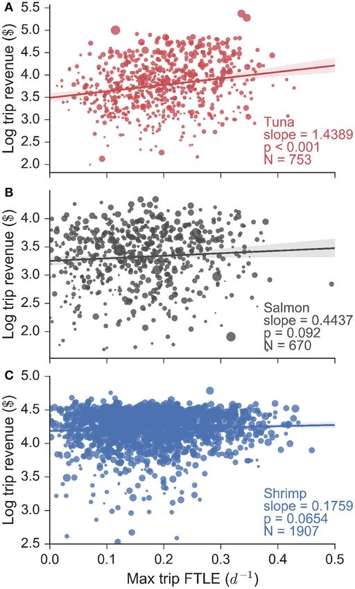
Watson et al. Fishing on Fronts
The choice of where to fish is in part determined by gradients and repulsion, typically calculated for the surface ocean, which
in ocean properties such as temperature, salinity, and pollution, identify frontal structures in advected tracers (d’Ovidio et al.,
that persist over timescales equivalent to or greater than those 2004; Lehahn et al., 2007). They have also been shown to
of a fishing trip (Lehodey et al., 1997). These often sharp correspond to biological activity. For example, it has been shown
gradients are created by fronts of various kinds, including that the spatial distribution of planktonic organisms (Harrison
buoyancy currents, tidal mixing, shelf-slope/shelf-break flow, et al., 2013), foraging frigate birds (Olascoaga et al., 2008),
upwelling and boundary currents, and marginal ice zone fronts. elephant seals (Della Penna et al., 2015), and baleen whales (Kai
Most fronts are characterized by a surface convergence, which et al., 2009), correspond with the location of LCSs. However,
contributes to the aggregation of nutrients and increases in while there exists evidence that fishing effort is colocated with
primary production (Kahru et al., 2012). As a consequence, LCSs (Prants et al., 2012), it remains unknown whether this is
ocean fronts collectively define a dynamic mosaic of transient a systematic relationship across different marine systems and
micro-habitats that numerous organisms use (MacKenzie et al., across fisheries, and also whether any relationship between LCSs
2004), and are known to be “hot spots" of marine life (Bost and fishing influences catch rates and the revenue generated by
et al., 2009; Godø et al., 2012; Scales et al., 2014; Woodson fishing.
and Litvin, 2015). Fronts are observable in satellite derived To understand whether fishermen track LCSs and whether
maps of sea surface temperature, primary production and ocean doing so has economic impacts, we compiled data on the
color. However, cloud cover, flow discontinuities and noise, location of over 1,000 fishing vessels every hour in the U.S.
and low spatial resolution of satellite data present challenges California Current Large Marine Ecosystem (CCLME) for the
for identifying the location of fronts (Ullman and Cornillon, period 2009–2013 produced from a Vessel Monitoring System
2000). To overcome these challenges, recent work has focused (VMS), and collated corresponding fisheries catch and price data.
on the spatiotemporal extent of fronts identified by Lagrangian We focused on the spatial dynamics of vessels operating in three
Coherent Structures (LCSs; frontal areas of convergence in commercially important fisheries: the albacore tuna (Thunnus
the surface ocean, see Figure 1 and Supplementary Movie; alalunga) troll, chinook and coho salmon (Oncorhynchus
Harrison and Glatzmaier, 2012). These are areas of attraction tshawytscha and Oncorhynchus kisutch respectively) troll and
pink shrimp (Pandalus jordani) trawl fisheries, which account
for roughly 35, 45, and 50 million US dollars in annual
revenue respectively (values from www.oceaneconomics.org/).
Complementing this, we gathered oceanographic information
for the same time period, from a 4-dimensional variational
(4D-Var) data-assimilation Regional Ocean Modeling System
(ROMS) solution to the US west coast (Moore et al., 2011a).
This ROMS model operates at a higher spatial and temporal
resolution than satellite altimetry data, which is commonly
used to answer similar questions, and assimilates as much
data as possible to make the best possible reconstruction
of past oceanic conditions for the U.S. West Coast. We
used the ROMS velocity fields to identify LCSs, and with
these data, we assessed whether fishing events from the tuna,
salmon and shrimp fisheries are associated with attracting
LCSs, and whether this impacts the revenue generated by
fishing.
METHODS
To assess the relationship between the spatial distribution of
fishing effort and the location of LCSs, we synthesized fisheries
landings data. Using these data we then defined fisheries for the
CCLME. Then, using spatially explicit vessel monitoring data
for the tuna, salmon and pink shrimp fisheries, we identified
fishing locations. In parallel to these analyses of fisheries data,
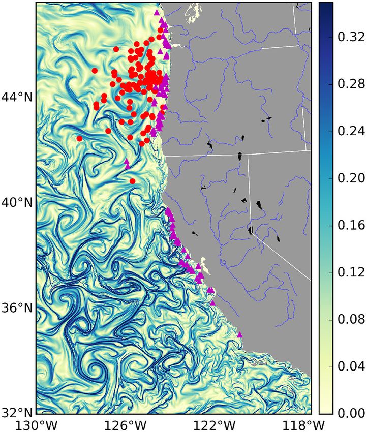
FIGURE 1 | Finite-time Lyapunov Exponent values (d−1 ) from the U.S. West
Coast on January 1st 2009. Strong frontal activity or—Lagrangian Coherent oceanographic data produced from a regional ocean model
Structures—are generally considered values > 0.1 d−1 . Overlaid are mock were used to identify LCSs in the CCLME for the same time-
locations of several fishing events for different fisheries: the tuna fishery in red period as covered by the fisheries data. Combining the two, we
and the salmon fishery in purple. Due to privacy restrictions we will not show assessed whether vessels, operating in different fisheries, appear
actual fishing locations, instead these are random points sampled from within
the 95% kernel density contour of each fishery.
to search for and catch fish preferentially on LCSs. The following
subsections expand on each of these steps.
Frontiers in Marine Science | www.frontiersin.org 2 February 2018 | Volume 5 | Article 46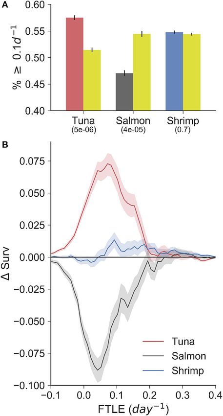
Watson et al.                                                                                                                     Fishing on Fronts

Identifying Fisheries from Landings Data                                   Linking Fishery Definitions to Vessel-Monitoring
Fisheries catch and price data were obtained from fish-tickets             System Data
compiled through the Pacific Fisheries Information Network                 In total, the fisheries trip data contained numerous fisheries. We
(PacFIN), and describe the time, location, catch and revenue of            subsetted these data and focused our analysis on the albacore
340,466 trips, spanning 5,980 vessels for the time period 2009–            tuna, salmon and pink shrimp métiers. Pacific albacore tuna
2013. Using these data, we identified fisheries as groups of similar       is a migratory species, caught relatively far from shore (see
trips based on what was caught. These trip-groups are otherwise            Figure 1: red dots) by towing artificial lures with barbless hooks
called métiers (mostly in Europe; Deporte et al., 2012). At its            or “trolling.” Of the three species we have studied, albacore tuna
heart, a métier analysis groups trips based on the gear used,              is the most likely to have a behavioral relationship with LCSs.
and the revenue and species composition of landings (Davie                 Indeed there is strong anecdotal evidence that tuna fishermen
and Lordan, 2011; Boonstra and Hentati-Sundberg, 2016). This               look for frontal features when trolling for tuna (gained from
methodology requires choices in the way similarity among trips             personal communications with tuna fishermen). The salmon
are measured, a clustering algorithm for grouping similar trips            fishery consists mainly of chinook and coho salmon, which
together, and scalability so that it can be applied to the 340,466         similarly to albacore tuna are caught by trolling, but are found
trips we had data for.                                                     mainly in areas closer to shore. Pink shrimp are associated
    The first step was to calculate the similarity of every pair of        with soft-sediment benthos, and are harvested by trawling nets
trips, measured using the Hellinger distance D (Legendre and               along the sea-floor. As a consequence, of the three focal species,
Legendre 2012). The Hellinger distance was calculated from the             they are the least likely to be affected by surface LCSs, which
species composition of two fishing trips A and B as follows:               will only impact the sea floor through the sinking of organic
                                                                           particles from phytoplankton blooms, which occurs over time-
                                  v
                                  u S                                      scales longer than considered here. Hence, we included shrimp
                                  uX                                       precisely because LCSs are expected to have no relationship.
                          DAB   = t (ai − bi )2 ,               (1)
                                                                               The locations of tuna, salmon and shrimp vessels were
                                       i=1
                                                                           obtained from a Vessel Monitoring System (VMS) dataset
                                                                           provided by the National Marine Fisheries Service’s Office of Law
where ai is the fraction of revenue derived from species i on trip         Enforcement (OLE). VMS is required for all vessels commercially
A, bi is the fraction of revenue derived from species i on trip            fishing federally managed groundfish in the past 5 years. Many
B, and S is the total number of species collected in both trips.           of these “groundfish” vessels operate in other fisheries and
Hence, as the difference in revenue attributable to each of the S          as a consequence the VMS data contained numerous tuna,
species increases, trips A and B become increasingly dissimilar.           salmon and shrimp trips. Vessel locations have an accuracy of
Applied to every pair of fishing trips results in a trip distance          approximately 500 meters and in total, we amassed 22 million
matrix.                                                                    GPS pings, hourly over the period 2009-2013, for 1,183 vessels.
    The next step was to transform the Hellinger distance matrix           However, no contextual data is provided with the VMS data, for
into a similarity matrix. This was done by subtracting each                example when a vessel is in port, when it is fishing, or what kind
element of the distance matrix from the maximum value of                   of vessel it is. As a consequence, the first challenge with these
the whole matrix. From this similarity matrix, we identified               data is to link them to the fisheries definitions obtained from the
métiers as groups of trips with similar target assemblages                 trip landings data, and then identify different spatial behaviors—
using the infoMap community detection algorithm (Rosvall and               searching for and catching fish vs. transiting—from the location
Bergstrom, 2008). This algorithm examines networks (which the              time-series.
similarity matrix represents, where nodes are trips and edges are              The first step to analyzing the VMS data was to identify trips.
trip similarity) for subgraphs more interconnected to one another          This was done in two steps. First, we assigned any VMS location
than the network in which it is embedded.                                  less than 1.5km from the shore and stationary for greater than
    Our dataset contained 340,466 unique trips, and due to                 3 hours as “in-port”. Distances to land were calculated using
computational limits, we were not able to implement the infoMap            NOAA’s GSHHG high-resolution geography dataset (Wessel and
algorithm using a single matrix containing all pairwise trip               Smith, 1996). This resulted in a subset of the VMS data that
similarities. To overcome this computational challenge, and                included only “at-sea” locations. Then, trip-times (time-out and
obtain manageable matrix sizes, we first performed the métier              time-in) from the fisheries landing ticket data were matched
analysis on one year’s worth of landings data, for example 2010.           with the at-sea VMS data points. This matching allowed us to
Then for each trip in other years (e.g., 2009, 2011, 2012, and             assign a unique index for sets of VMS data-points associated with
2013), we identified which 2010 trip was “nearest” to it, in terms         a distinct fishing trip. Furthermore, once the fisheries analysis
of species composition, using a k-nearest neighbors algorithm.             of the landing ticket data was performed, we were also able to
Each trip in 2009, 2011, 2012, and 2013 then inherited the métier          assign a fishery to each trip in the at-sea VMS data. Doing so
of its nearest 2010 trip. In this way, we managed to assign                identified what species was being harvested on each trip in the
all trips from the whole dataset to specific métiers. We tested            VMS database.
this method using different “base” years (i.e., different to 2010              The last step was to link a NOAA Fisheries West Coast
in the above example), and found our results robust to this                Groundfish Observer Program data to the at-sea VMS data,
decision.                                                                  for the purpose of validating the spatial behavior segmentation

Frontiers in Marine Science | www.frontiersin.org                      3                                       February 2018 | Volume 5 | Article 46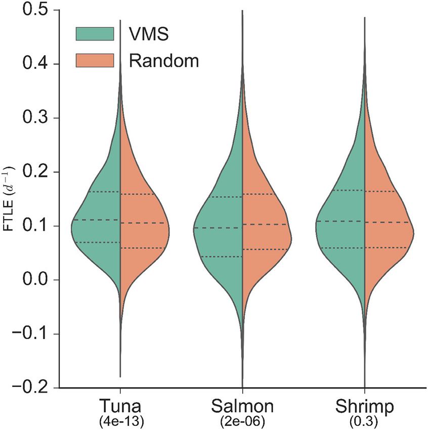
Watson et al.                                                                                                                                     Fishing on Fronts

(i.e., identifying when a vessel was fishing or not). This involved       Lee, 2012), and although supervised classification methods are
matching vessel identifiers and time-points in each database.             available (Joo et al., 2015), and access to the NOAA observer
These observer data included descriptions of the vessel, the              data meant we had the means to construct and test them, there
location, and time-in and -out of a fishing set (i.e., the time           are several caveats to the observer data (see paragraph below),
when fishing happened) for 8,932 trips spanning 334 vessels over          and ultimately we would only be able to develop supervised
the period 2009–2013. We identified which at-sea VMS data                 methods for a small subset of fisheries due to data restrictions.
points lay within these set-in/set-out time-spans, and used this          Furthermore, these supervised classification methods would
information in validating the behavioral segmentation algorithm           perform poorly for those fisheries to which they could not be
described below. Importantly, the NOAA observer data only                 trained (i.e., the tuna and salmon fisheries). As a consequence,
covered a fraction of the trips in the at-sea VMS data, for example       we used a simple unsupervised approach based solely on speed
13% of shrimp trips.                                                      that could be applied across fisheries. We used the NOAA
                                                                          observer data post-hoc to calculate the precision of our method,
                                                                          and we found it to perform well for all fisheries for which
Vessel Monitoring System Data Behavioral                                  we could validate, averaging 83% (see Table 1; precision was
Segmentation                                                              calculated from the frequency of true-positives—locations that
The at-sea VMS data remained a collection of lat/lon time-                both the NOAA observer data and our algorithm identified as
series, grouped by trip and fishery. In order to identify when and        fishing.). Importantly, we accounted for the precision of our
where fishing occurred from these time-series, we developed an            classification method using bootstrap methods in all subsequent
unsupervised behavioral segmentation algorithm, which works as            statistical analyses, meaning our results are robust to the
follows. Vessel speed was calculated as the distance traveled per         choice of using a simple unsupervised behavioral segmentation
unit time between sequential location pings for all trips, making         method.
sure to also calculate the spatial mid-point between consecutive              Another challenge that we came across, that affected our
lat/lon points. Furthermore, for each trip, checks were made for          decision to use an unsupervised classification scheme, was
extreme and unrealistic speeds. Then, for each vessel we subsetted        systematic error in the start and end times of fishing in the
trips by fishery, and calculated empirical speed distributions.           NOAA observer data. For example, in Figure S2 we show a
To these empirical distributions we fitted Gaussian Mixture               mock fishing trajectory where colored dots identify a fishing
Models (GMM), varying in the number of components (i.e.,                  vessel’s location, and the color the speed. We cannot show the
modes) modeled. The “best” model was selected using Bayesian              tracks of a real fishing trajectory, but this mock-up copies exactly
Information Criterion. The last step was to identify the 50th             a problem seen throughout our data. Specifically, the NOAA
percentile value of the first Gaussian component of the best              observer set-in and set-out dates identify VMS locations that
model. This speed value was used as a cut-off: any locations              are not likely fishing events. In the top-panel of Figure S2, the
with speeds less than or equal to this value were assumed to              dots surrounded by a grey-circle identify those VMS locations
be fishing-intended or fishing activity. This speed identifies the        identified as fishing by the observer data. It is obvious that
where the first component (i.e., fishing) becomes less likely             the observer data suggest this vessel is fishing, while steaming
than the second component (i.e., steaming). As an example,                fast away from the true fishing location (the knot of points in
Figure S1 shows the empirical speed distributions, the best               blue). In contrast, our speed algorithm identifies what by eye
GMMs, and the cut-off speeds for a vessel that participated in            are likely the true fishing locations (gray circles in the bottom
a tuna, salmon and shrimp trip. All locations with speeds less            panel of Figure S2). This potential error in the NOAA observer
than or equal to the cut-off, for that specific type of trip and          data contributed to our decision not to develop a supervised
for that vessel, were assumed to be fishing or fishing-intended           classification scheme.
events.
    Vessel-speed criteria are commonly use to infer whether a
VMS record corresponds to fishing activity (Murawski et al.,              TABLE 1 | The precision of the VMS segmentation algorithm, applied to different
2005; Eastwood et al., 2007; Lee et al., 2010; Gerritsen and              métiers that we had NOAA observer data for.
Lordan, 2011). For example, vessel speeds are commonly used to
                                                                          Common Name                                          N                          Precision
determine when trawling is in progress, with 8 knots considered
to represent the upper limit of trawling speed for North Sea              Sablefish (longline)                                756                           0.659
beam trawlers (Dinmore et al., 2003). Some authors who have               Sablefish (pot)                                     277                           0.884
used a similar approach have reported a significant number                Dungeness crab (pot)                                 78                           0.962
of false-positive results (where vessels were traveling at fishing        Dover sole (trawl)                                 5626                           0.828
speeds, but were not actually engaged in fishing). However,               California halibut (trawl)                           62                           0.516
false-negative results tend to be rare. Indeed, previous work has         Pacific pink shrimp (trawl)                        1651                           0.732
included directionality in addition to speed, as determinants of
fishing, but they only resulted in a very small improvement               Precision is the fraction of VMS-fishing behaviors that were actually fishing events (i.e.,
                                                                          true positives). The reasonable level of precision of our algorithm, across this broad range
on speed alone (Mills et al., 2007). Further, unsupervised
                                                                          of metíers, meant we were confident of its use for the tuna and salmon (for which we had
behavioral segmentation algorithms like ours are commonly used            no observer data) and shrimp metíers. The average precision of the algorithm (83%) was
(Murawski et al., 2005; Gerritsen et al., 2012; Jennings and              used in the subsequent analyses.

Frontiers in Marine Science | www.frontiersin.org                     4                                                     February 2018 | Volume 5 | Article 46
Watson et al. Fishing on Fronts Oceanographic Data provided online here http://oceanmodeling.ucsc.edu/. Examples The spatial distribution of attracting LCSs for the whole U.S. of the SST and surface velocity fields produced by the ROMS California Current Large Marine Ecosystem, for the period 4D-Var data assimilation system are shown in Figure S5, which 2009-2013, was estimated using modeled surface ocean currents should be compared to empirical observations for the same produced from a 4-dimensional variational (4D-Var) data day shown in Figure S3 (surface temperature) and Figure S4 assimilation Regional Ocean Modeling System (ROMS) solution (surface chlorophyll) for a qualitative verification of its ability to (Haidvogel et al., 2000, 2008; Shchepetkin and McWilliams, reproduce past ocean conditions. 2003, 2005). The ROMS model and domain is described in detail elsewhere (Moore et al., 2011a) so only a brief Lagrangian Coherent Structures description is given here. The domain spans the region 134◦ W Using the ROMS modeled surface velocities, we identified the to 116◦ W and 31◦ N to 48◦ N, extending from midway down location of LCSs through time (Castruccio et al., 2013). These the Baja Peninsula to Vancouver Island at 1/10 degree (roughly flow features are material curves that map filamentation and 10 km) resolution, with 42 terrain-following levels resolving transport boundaries (Harrison et al., 2013). Fluid particles vertical structure in ocean properties. We chose to use surface straddling a LCS will either diverge (repelling LCS) or converge currents from the high-resolution ROMS reanalysis to identify (attracting LCS) in forward time (Haller and Yuan, 2000). LCSs and corresponding fronts, instead of geostrophic velocity LCSs thus delineate the boundary between dynamically distinct fields derived from satellite altimetry used in several previous regions of the flow field, effectively allowing us to visualize studies of LCSs. We made this choice for several reasons: the skeleton of turbulent transport (e.g., Haller, 2002; d’Ovidio (i) the altimetry-based approach cannot be applied reliably et al., 2004; Shadden et al., 2005). Whereas the resolution of in coastal regions, where the geostrophic balance no longer the ROMS velocities may appear relatively coarse compared holds because of strong lateral and bottom boundaries and to the spatial scales of fishing, the topological structure nearshore forcing; (ii) geostrophic surface currents derived of surface ocean LCSs has been shown to be robust to from satellite altimetry are only available at coarser spatial noise and low spatial resolution velocity fields (Harrison and resolution (at 1/4o or roughly 25 km in our domain); (iii) Glatzmaier, 2012). The spatial organization of LCSs has a altimetry accuracy decreases near the coast, where much fishing large impact on the coastal environment not only because occurs, due to measurements being affected by the presence they influence the dispersion of tracers in the water but of land in the satellite footprint (i.e.,
Watson et al.                                                                                                                       Fishing on Fronts

equal to the grid spacing. The final separation δt is computed              random-FTLE points greater than or less than 0.1 d−1 , which
as the maximum separation after a particle advection time of 10             is a threshold value that corresponds to frontogenesis timescales
days, which is the typical mesoscale eddy-turnover time in the              faster than 1 month—a time span that has been shown to be
region. Large FTLE values identify regions where the stretching             ecologically significant, attracting numerous taxa (d’Ovidio et al.,
induced by mesoscale and submesoscale activity is strong and are            2004; Olascoaga et al., 2008; Kai et al., 2009).
typically organized in convoluted lines encircling submesoscale                 We repeated this statistical comparison of VMS-FTLE and
filaments. A line of local maxima of FTLE (more precisely, a                random-FTLE distributions, using a different random test. Here,
ridge) can be used to predict the location of tracer fronts induced         instead of choosing random points from within the 95% contour
by horizontal advection and stirring; in other words, the location          of each fishery, we chose them randomly from within the whole
of LCSs. A snap-shot of the spatial distribution of backward                U.S. CCLME domain. Like the fishery-specific random test, we
FTLE values and the complementing probability distribution                  performed Kolmogorov-Smirnov tests and G-tests of goodness-
are shown in Figure 1 and Figure S6 respectively. Further, an               of-fit.
animation showing the dynamic nature of FTLE fields is provided                 In addition to testing whether fishing was randomly associated
in the Supplementary Movie. These maps and the animation                    with high FTLE values and LCSs, or not, we also explored
highlight the complex spatial patterns exhibited by LCSs (large             whether fishing on high FTLE values impacts the revenue
FTLE values), and the probability distribution shows that FTLE              generated by a trip. To do so, we performed linear univariate
values are roughly log-normally distributed, with a mode around             regression analysis and fit linear mixed models with the
0.1d−1 . The LCS’s ability to outline observed tracer patterns in           maximum VMS-FTLE value per trip as the explanatory variable,
geophysical flows is well illustrated by Figure S5 where LCSs               and trip-revenue as the dependent variable. In the case of the
align with frontal structures and filamentation in temperature.             linear mixed models, vessel length was additionally included as a
                                                                            fixed effect, and vessel-ID as a random effect. In order to estimate
                                                                            the significance of the regression parameters, we bootstrapped
Statistical Analysis of Fishing and                                         these analyses by taking only 83% of values, reflecting the
Lagrangian Coherent Structures                                              expected behavioral segmentation precision, and repeating the
The behaviorally segmented VMS data consists of a list of                   regression analyses 1,000 times. This bootstrap approach allowed
locations where fishing or fishing-intended activities occurred             us to estimate a distribution and p-value for each regression
over the period 2009-2013. In total, these data included 3233               parameter (i.e., the slope).
tuna, 2201 salmon and 7762 shrimp fishing locations. We then
linearly interpolated in space and time the FTLE data, produced
from the ROMS modeled velocity data, to these locations. The                RESULTS
result is a unique FTLE value per fishing location. The next step
was to generate a null dataset with which to compare VMS-                   The VMS-FTLE and random-FTLE distributions for the tuna,
FTLE values. Following the approach of (Cotté et al., 2011), for            salmon and shrimp fisheries are shown in Figure 2. Values range
every fishing location estimated from the VMS data, a random                from past −0.1 day−1 to 0.5 day−1 , with median values for
location was chosen from within the 95% kernel polygon of                   each fishery all around 0.1 day−1 . From these violin plots it
the fishing location’s parent fishery (see Figure S7 for maps               is possible to identify systematic qualitative differences between
showing the spatial distribution of fishing effort for each fishery).       the VMS-FTLE and random-FTLE values. For example, for the
The kernel density estimation was performed on each fishery’s               tuna fishery the VMS-FTLE median, 25th and 75th percentiles
fishing locations only, and results often identified numerous               are all greater than the corresponding random-FTLE values.
distinct polygons. In this case, random points were created by              The Kolmogorov-Smirnov tests identified that the tuna and
first choosing a polygon probabilistically, in proportion to its            salmon VMS-FTLE distributions are significantly different from
area, and then a choosing a location randomly from within                   random, but that there is no significant difference between the
that polygon. FTLE values were then linearly interpolated in                shrimp VMS-FTLE and random-FTLE distributions (Figure 2;
space and time to each random point. The result is a set of                 Kolmogorov-Smirnov p-values are given below the fishery
random points in the “preferred fishing region” of each fishery.            names). In addition, we found that for the tuna, salmon and
These random-FTLE distributions were then compared with the                 shrimp fisheries respectively, 57, 47.5, and 55% of fishing events
corresponding VMS-FTLE distributions.                                       happen on FTLE values ≥ 0.1day−1 , relative to 52, 50.5, and
    In order to explore differences between the VMS and random-             54% of random events (see Figure 3A). The G-test p-values
FTLE distributions, we performed Kolmogorov-Smirnov tests                   reflect those from the Kolmogorov-Smirnov tests, that is the
and G-tests of goodness-of-fit. The Kolmogorov-Smirnov test                 fraction of fishing events occurring on FTLE values ≥ 0.1day−1
quantifies the significance of the largest difference between two           in the tuna and salmon fisheries are significantly different from
cumulative density functions, whereas the G-test quantifies the             random, whereas in contrast, there is no significant difference
significance of the difference in the frequency of particular               for shrimp fishing. The differences between the VMS- and
events. Both Kolmogorov-Smirnov and G-tests were repeated                   random FTLE values, for the tuna fishery, are 2–3 times less
1,000 times, subsampling 83% of the VMS- and random-FTLE                    than those observed for foraging baleen whales (Cotté et al.,
distributions to reflect the behavioral segmentation precision.             2011) (the fraction of baleen whales found on FTLE values
For the G-test, we calculated the frequency of VMS- and                     greater than 0.1day− 1 was roughly 10–15% greater than would

Frontiers in Marine Science | www.frontiersin.org                       6                                        February 2018 | Volume 5 | Article 46
Watson et al. Fishing on Fronts
FIGURE 2 | Distributions of backward finite-time Lyapunov exponent values
from VMS (left of axis/green) and random (right of axis/orange; sampled from
within the 95% density contour of each fishery) locations. Median values are
identified by the dashed lines, and upper and lower quartiles are identified by
the dotted lines. Kolmogorov-Smirnov p-values are indicated below fishery
names, indicating the significance of the difference between the VMS- and
random-distributions (i.e., only the shrimp fishery VMS-FTLE distribution is not
significantly different from random).
be expected at random). This suggests that tuna fishermen are
not tracking these surface frontal features as closely as baleen
whales.
To highlight the way in which these distributions differ from FIGURE 3 | (A) Bar-plot showing the fraction of fishing (red-tuna,
gray-salmon, blue-shrimp) and random (gold; sampled from within the 95%
random, we calculated the difference in VMS- and random- density contour of each fishery) points with a FTLE value greater than or equal
FTLE survival functions, 1surv, bootstrapping values with an to 0.1d−1 . G-test p-values are shown below each fishery label. (B) The
83% sample size to create confidence intervals that reflect the difference in VMS- and random-FTLE survival functions (1Surv) for the three
behavioral segmentation precision (in the case for shrimp, for fisheries with 95% confidence intervals. These curves highlight that tuna
fishermen search for and catch fish in areas of the ocean with FTLE values
which we had fishing observations, we used 75% precision: see
greater than would be expected by chance. In contrast, salmon fishermen are
Table 1). Survival functions identify the fraction of points with found preferentially in areas with low FTLE values.
a certain FTLE value or greater (formally, they are 1 minus a
cumulative density function), and the difference between the
VMS- and random-survival functions identifies the magnitude
and type of non-random association fishermen have with LCSs. resolution of the ROMS model, from which the FTLE data were
For example, from the 1surv curves shown in Figure 3B, it is calculated, is not sufficient to resolve the physical features that
evident that tuna fishing events always occur on FTLE values salmon fishermen use to locate salmon. This is an important
greater than would be expected from random, that is the red caveat to this work, and is expanded upon in the discussion.
curve is always positive over the entire range of FTLE values. This Third, salmon fishing may occur in places where LCSs were
strongly suggest that tuna fishermen preferentially search for and recently. We do not account for the possible time-lag between
catch tuna on LCSs, as quantified by FTLEs. fishing and the presence of an LCS, but we can hypothesize
In contrast to tuna fishing, salmon fishing always occurs that a time-lag would only happen if salmon track some
on FTLE values less than would be expected from random, trailing effect of LCSs. This is clearly possible, as the ecosystem
that is 1surv values are negative. This can be interpreted effects of fluid convergence, caused by LCSs, will be integrated
in three ways. First, salmon fishermen may search for and over space and time. In contrast to both tuna and salmon
catch fish in specific areas of the coast that have reduced fishing, there is less difference between the shrimp VMS- and
frontal activity relative to nearby waters. Second, the spatial random-survival functions. In general, the shrimp 1surv curve
Frontiers in Marine Science | www.frontiersin.org 7 February 2018 | Volume 5 | Article 46Watson et al. Fishing on Fronts
hugs the zero-line (the point at which there is no significant
difference to random). Hence, when combined with non-
significant p-values from the Kolmogorov-Smirnov and G-tests,
this information confirms our expectation that shrimp fishing
has no spatial correspondence with LCSs and surface frontal
features.
The results of the whole-domain random test contrast strongly
with those produced from the fishery-specific random test
(compare Figure 3 and Figure S8). Here, all fisheries—tuna,
salmon and shrimp—show negative 1surv curves. This identifies
that each of these fisheries operates in areas of the California
Current with low FTLE values relative to the rest of the domain. It
is an interesting oceanographic question to ask why this happens,
but because our focus is on the spatial relationship between
individual fishing events and specific FTLE features, and not
with LME-scale biophysical patterns, we do not answer it in
this paper. One point to note is that the qualitative differences
between the 1surv curves of each fishery are consistent across
the fishery-specific and whole-domain tests. That is, the tuna
curve is the least negative, the shrimp curve is an intermediate
case and the salmon curve is the most negative. This qualitative
consistency reflects the results of the fishery specific tests (i.e., that
tuna fishermen track FTLE values that are relatively high when
compared to shrimp and salmon fishermen).
These FTLE statistics reveal that tuna fishermen preferentially
search for and catch fish in areas of high oceanic filamentation,
in other words areas of the ocean with strong fronts. In contrast
salmon fishing occurs in areas of low filamentation, and shrimp
fishing occurs independently of the FTLE context. Do these
behaviors translate into economic terms for fishermen? In order
to answer this question we assessed the relationship between
total revenue gained per trip (in log10 $) and the maximum
FTLE value experienced whilst fishing, for every trip for each
fishery (Figure 4). Our data consisted of 753 tuna, 670 salmon
and 1907 shrimp trips (made by 94, 69, and 56 unique vessels
FIGURE 4 | Logarithmic trip revenue (log$) as a function of the maximum
respectively), and we found that for tuna fishing, there is finite-time Lyapunov exponent (FTLE) experienced while fishing on a particular
a significant positive linear relationship between logarithmic trip, for all (A) tuna, (B) salmon, and (C) shrimp fisheries. Marker size is
trip revenue and the maximum FTLE value experienced while proportional to vessel length. We find a significant linear relationship for tuna
fishing. The slope of this linear relationship is 1.44 log$ per fishing trips, indicating that tuna fishermen make more money the more they
fish on fronts. This is confirmed using a linear mixture model that accounts for
unit FTLE (with a standard error of 0.12 log$ per unit FTLE, the effect of vessel size. Both the salmon and shrimp trips show flat and
calculated from bootstrapping the regression and subsampling non-significant relationships.
the data by 83% to account for the segmentation precision).
This univariate analysis implies that a tuna vessel that searches
for and catches fish on a front with FTLE value 0.1 d−1 can
be expected to make roughly $3,500 on a single trip, while a Vessel size plays a role in determining trip revenue (Figure 4:
vessel that catches fish on a front with FTLE value 0.4 d−1 marker size is proportional to vessel length), because larger
is expected to make $10,000 on a single trip, roughly three vessels have more storage space and hence a greater capacity
times the revenue. Flat and non-significant relationships were for bringing fish to harbor. Using generalized linear mixed
observed for salmon and shrimp trips indicating that trip revenue models (bootstrapping results using subsamples similar to the
in these fisheries are not affected by the FTLE conditions univariate analysis) we indeed found that vessel size and tuna
experienced while fishing. These results are mirrored when revenues are strongly and positively correlated (slope = 1.805,
trip revenue is substituted by trip landings (in units of mass: p-value < 0.001). However, we still also found a positive
Figure S9), but they are not found when the expected FTLE and significant (albeit secondary) effect of FTLE values on
experienced whilst fishing is used in place of the maximum trip revenue (slope = 0.582, p-value < 0.001). In contrast,
(Figure S10; this highlights that the maximum FTLE experienced vessel size and FTLE values were not important determinants
while fishing on a given trip is a better measure of catch of salmon (slopes = 0.588, 0.344; all p-values > 0.05) or shrimp
success). (slopes = −0.001, 0.369; all p-values > 0.05) trip revenues.
Frontiers in Marine Science | www.frontiersin.org 8 February 2018 | Volume 5 | Article 46Watson et al. Fishing on Fronts
DISCUSSION that persist over timescales of roughly less than a month. If we
were to have used higher spatial resolution data, we would have
Our results have identified a connection between fine-scale assessed the impact of even finer spatial scale and potentially
physical ocean features and the spatial patterns of human more ephemeral physical ocean features on fishing. Importantly,
activity, and ultimately the economic welfare of fishermen. at some fine scale there will cease to be any relationship. This
Specifically, our results infer that fishermen targeting albacore is the spatial and temporal scale at which fishermen no longer
tuna track LCSs, as identified by large backward Finite-time are able to sense and react to the seascape. It is an interesting
Lyapunov exponents. This is reflected in the location of tuna question to ask at what scale this is, and it likely relates to the
fishing events, which are consistently found on LCSs, more so technology that fishermen employ to search for fish. Because it is
than would be expected at random, and also in the revenue related to technology, this minimum spatiotemporal scale is likely
gained by tuna fishermen. That there is significant positive decreasing, as vessels improve in speed and sensory ability.
correspondence between the spatial distribution of fine-scale In contrast to examining finer scale behaviors, one could
(and ephemeral) physical features of the ocean and the income coarse-grain the (ROMS) data, and assess the relationship
of fishermen is surprising, for there are many possible reasons between fishing and aggregate measures of the seascape. These
why one fisherman might make more money than another coarse graining experiments have been used to examine the
(Fulton et al., 2011). For example, the institutional context, skill relationship between pelagic predators and relatively large areas
and experience, gear and weather all play a role in how much of the ocean, characterized by different biophysical properties
money a fishermen might make on any given trip (Hilborn, (Scales et al., 2017). Coarse graining experiments like these move
1985; Bjarnason and Thorlindsson, 1993; Allison and Ellis, 2001). the focus away from the behavior of individual fishermen and
Thus, the clear signal of the physical ocean environment—the fishing vessels, and instead ask questions about where groups
seascape—in the revenue garnered by tuna fishermen highlights of vessels (fleets) operate. This is a vital consideration because
the potential for strong natural-human coupling in the California while management typically focuses on directing the behavior of
Current system. individual humans, their performance is often measured at the
In contrast to tuna fishing events, we observed a negative fleet level (Hilborn, 2007), and fleets themselves vary in their
relationship between salmon fishing and FTLE values, and no composition and in where their aggregate effort is directed (e.g.,
relationship for shrimp fishing. The absence of any relationship Figure S7;Boonstra and Hentati-Sundberg, 2016).
for shrimp fishing was expected, as shrimp fishing targets the An important aspect of fisheries management that this
benthos (Eales and Wilen, 1986), and as a consequence the study relates to is the impact of LCS-focused foraging on the
surface physical structures described by FTLE values would organization and dynamics of the underlying marine food-web
not be expected to have an impact. However, the negative (Woodson and Litvin, 2015). Spatially focused foraging and
relationship seen in salmon fishing raises an important caveat consumption has been shown to impact fish stocks through
of this work. It is impossible to tell whether this observation a phenomenon known as “local depletion” (Bertrand et al.,
arises from an actual avoidance behavior of salmon fishermen, 2012), and in ecology these non-linearities in predator-prey
or whether this simply arises due to the inability for the ROMS interactions change the long-run mortality rate of prey, and
model to resolve ocean processes close to shore, which is where the population growth rate of predators (Fryxell et al., 2007).
salmon fishing typically occurs (see Figure 1). Although at the This is important because the ecosystem models that we
time of this work, the ROMS model data has a finer spatial currently employ to quantify and predict the dynamics of marine
resolution than satellite data, which is typically used to assess ecosystems (e.g., Watson et al., 2015), possibly in the context of
the impact of LCSs on predator foraging (e.g., Kai et al., 2009; evaluating the potential response of management changes, use
Cotté et al., 2011; Della Penna et al., 2015), it is still too coarse to very simple linear mathematical functions to represent predator-
resolve coastal zone processes, which likely include even finer- prey encounter rates (e.g., the numerator in a Type II feeding
scale physical ocean features than the LCS assessed here. For function). These linear functions assume that prey are uniformly
example, the FTLE value of 0.1d−1 that we used has been adopted distributed over a given area, and predators move randomly over
in previous works studying the relationship between marine this area (Barbier and Watson, 2016). We know that in reality
top-predators and LCSs (e.g., Cotté et al., 2011). But these studies that this is not so, and our analysis confirms this. It is fair to say
all focused on ocean regions far from shore (at least several tens that all models are abstractions of reality; however, it is important
of kilometers). Most likely, a different FTLE value will identify to know the effect of these simplifying assumptions on the
dominant frontal features in coastal zones. Hence, while 0.1d−1 predictive skill of our ecosystem models. Our analysis suggests
is appropriate for tuna fishing which occurs relatively far from that more sophisticated predator-prey encounter functions that
shore, for studying the spatial behavior of vessels operating closer account for spatially focused foraging, and other important
to shore, a different value should be identified using new higher factors such as cooperation and advanced fishing technologies,
resolution oceanographic information. are likely to provide new insights into fisheries dynamics (Fulton
Indeed, the spatial scale at which fisherman behavior is et al., 2011; Barbier and Watson, 2016).
assessed is a critical choice on the part of the investigator (Levin, One major policy tool that will benefit from improved
1992). Our choice to use the ROMS modeled data (produced understanding of the fine-scale spatial behavior of fishermen is
at a spatial resolution of roughly 10km) allowed us to assess marine spatial planning. Marine spatial planning takes many
the impact of physical ocean features at this same spatial scale, forms, for example Marine Protected Areas (MPAs) which have
Frontiers in Marine Science | www.frontiersin.org 9 February 2018 | Volume 5 | Article 46Watson et al. Fishing on Fronts
been widely adopted around the world (Edgar et al., 2014), and impending shifts in species ranges expected with climate change
define areas of the ocean that are off-limits to fishing. Obviously, (Pinsky et al., 2013). Furthermore, incorporating fine spatial-
because vessels operating in different fisheries search for and scale information into management policies is essential if we
catch fish in different places, MPAs will have a varying impact are to continue to improve the efficiency of fisheries (Hobday
on people’s income, depending on which fisheries they work in. et al., 2011). Increased fisheries efficiency would lead to fishermen
Knowing in which oceanic regions and at what times of the year spending less time at sea, and as a consequence reduced risk
different fisheries operate is key to designing MPAs efficiently of harm. Of course, in the interest of long-term sustainability
(Le Pape et al., 2014). Further, there are more sophisticated this increase in efficiency should be matched by changes in
approaches to marine spatial planning, for example temporary governance institutions that prevent over harvest. Ultimately,
closures (Brown et al., 2015), and policies directed at specific given the coupled nature of social-ecological systems, integrating
spatial behaviors, for example bycatch move-on rules (Dunn high resolution data on physical, chemical, ecological and social
et al., 2014). Like MPAs, improved understanding of the spatial factors will improve both how and to what extent we use living
behavior of fishermen, at fine spatial and temporal resolution, will natural resources (Wilen, 2004), leading to improved chances of
be critical to advancing these arguably more sophisticated forms prosperity now and in the future.
of marine spatial planning.
Marine spatial planning extends to other ocean-industries, not AUTHOR CONTRIBUTIONS
just fishing. Indeed, much applied research is currently focused
on “cross-sector” marine spatial planning, which aims to develop JW, EF, FC, and JS all contributed data, designed the scientific
policies that optimize the (sustainable) use of the oceans by all approach, analyzed the data and wrote the manuscript.
sectors, for example fishing, aquaculture, shipping, tourism and
oil and mineral extraction (Lester et al., 2013; Klinger et al.,
2017). Like in the case of marine spatial planning geared solely FUNDING
for fisheries (e.g., MPAs), cross sector spatial policies will depend
JW and EF acknowledge the support of the NSF Dynamics of
on a detailed quantification of spatial behavior. Importantly,
Coupled Natural-Human Systems grant GEO-1211972 and NSF
this advanced understanding will not only improve our ability
GRFP: DGE-1148900 respectively.
to design cross-sector policies for optimal/sustainable use of
multiple ocean resources, but it will help us anticipate how people
(like fishermen) will respond to these new policies (Klein et al., ACKNOWLEDGMENTS
2017). This is key to developing cross-sector policies that will
provide opportunities for (economic) growth in the long-run, as We would like to thank Frank Davenport, Claudie Beaulieu
the social and ecological organization of marine systems change for their help in preparing this manuscript. We would
(Klinger et al., 2018). especially like to thank Brad Stenberg and the Pacific Fisheries
A final consideration for integrating detailed understanding Information Network (PacFIN), the Pacific States Marine
of fishing spatial behavior into marine management is that Fisheries Commission, Kelly Spalding and the VMS Program
fishermen typically work in numerous fisheries over a given at the National Marine Fisheries Service’s Office of Law
year (Kasperski and Holland, 2013; Fuller et al., 2017). As a Enforcement, the NWFSC Observer Program, and Chris
consequence, fishermen will move across, exploit and make Edwards at UC Santa Cruz for providing the ROMS data. We
money from different parts of a seascape at different parts of also thank the Washington, Oregon and California Departments
the year. Hence, they will have many relationships with different of Fish and Wildlife for sharing their data.
parts of the seascape. For example, a fisherman on the U.S. west
coast that works in the albacore tuna fishery may also work in SUPPLEMENTARY MATERIAL
the dungeness crab fishery. As a consequence, high FTLE ocean
features will be important to this fisherman during the tuna The Supplementary Material for this article can be found
season, but not when they operate in the crab fishery. This is online at: https://www.frontiersin.org/articles/10.3389/fmars.
similar to agriculturalists that grow different crops in different 2018.00046/full#supplementary-material
parts of a landscape at different parts of the year. Indeed, just like Figure S1 | The probability density function of speed from (A) tuna, (B) salmon,
in agricultural management (Iverson et al., 2014), spatial marine and (C) shrimp trips. Empirical distributions are shown in gray, the “best” fitted
policies will be improved if they acknowledge that fishermen’s Gaussian Mixture Models in orange, and the cut-off speeds that are used to
segment fishing and non-fishing behaviors is identified by the blue dashed line.
diverse harvest portfolios connect different parts of seascapes
(Hobday et al., 2011). Figure S2 | A mock-example of one trip. We are not allowed to show real fishing
trajectories due to privacy constraints, so instead we created this mock-up based
In summary, coastal management and marine spatial planning
on a real example. Fishing vessel locations are identified by the colored dots (each
that recognizes and accounts for feedbacks between fishermen separated by 5 min.) and speed (m/s) is identified by color. For this particular trip
behavior and the dynamic and structured nature of seascapes is there are two searching/fishing events, identified by the clusters of slow-speed
likely to meet with greater compliance and provide for stronger points. One problem we identified was that the NOAA observer data can
resilience in the face of cumulative anthropogenic impacts. sometimes be obviously erroneous. This is explained in the (Top), where the VMS
locations circled in gray identify when the NOAA observer recorded that fishing is
Indeed, flexibility and resilience—the ability to cope with change happening. For the top-most fishing event, there is clearly an overshoot. In
(Folke, 2006)—are key properties of coastal human communities contrast, our behavioral segmentation approach (Bottom) based on vessel speed
that managers are looking to bolster, especially in the context of is much more conservative.
Frontiers in Marine Science | www.frontiersin.org 10 February 2018 | Volume 5 | Article 46Watson et al. Fishing on Fronts
Figure S3 | Observed sea surface temperature provided by the Operational Sea Figure S8 | Statistical analysis produced from the “whole-domain” random rest.
Surface Temperature and Sea Ice Analysis (OSTIA, Donlon et al., 2012). OSTIA (A) Bar-plot showing the fraction of fishing (red-tuna, blue-shrimp, gray-salmon)
uses satellite data provided by the GHRSST project, together with in-situ and random (gold) events with a FTLE value greater than or equal to 0.1d1 . G-test
observations to determine the sea surface temperature. The analysis is produced p-values are shown below each fishery label. (B) The difference in VMS- and
daily at a resolution of 1/20o (approximately 5 km). random-FTLE survival functions (1 Surv) for the three fisheries with 95%
confidence intervals.
Figure S4 | Observed chlorophyll concentration (Maritorena et al., 2010) for May
23rd 2010, made using Level 3, daily, binned imagery from SeaWiFS, Figure S9 | Logarithmic trip landing (log10 lbs) as a function of the max finite-time
MODIS-Aqua, and Meris. Lyapunov exponent experienced while fishing on a given trip, for all (A) tuna, (B)
salmon, and (C) shrimp trips. We find a significant linear relationship for tuna
Figure S5 | ROMS 4D-Var posterior estimate of Sea surface temperature (color
fishing trips, indicating that tuna fishermen make more money the more they fish
shading) and surface velocity (vector) for May 23rd 2010. Attracting Lagrangian
on strong filaments. Both the salmon and shrimp trips show now (significant)
Coherent Structures (LCSs) are ridges of the Finite-time Lyapunov Exponent
relationships. Marker-size is proportional to vessel length.
(FTLE) field, and are identified by the white lines.
Figure S10 | Logarithmic trip revenue (log$) as a function of the expected
Figure S6 | Probability density function of finite-time Lyapunov values on Jan 1st
finite-time Lyapunov exponent (FTLE) experienced while fishing on a particular trip,
2009, for the ROMS US west coast modeled domain.
for all (A) tuna, (B) salmon, and (C) shrimp fisheries. Marker size is proportional to
Figure S7 | Fishing intensity (log10 fishing days) for the tuna, salmon and shrimp vessel length. We find no significant linear relationships for any of the fisheries
métiers, calculated from the VMS data over the period 2009–2013. studies.
REFERENCES d’Ovidio, F., Fernández, V., Hernández-García, E., and López, C. (2004). Mixing
structures in the mediterranean sea from finite-size lyapunov exponents.
Allison, E. H., and Ellis, F. (2001). The livelihoods approach and Geophys. Res. Lett. 31:L17203. doi: 10.1029/2004GL020328
management of small-scale fisheries. Marine Policy 25, 377–388. Dunn, D. C., Boustany, A. M., Roberts, J. J., Brazer, E., Sanderson, M., Gardner,
doi: 10.1016/S0308-597X(01)00023-9 B., et al. (2014). Empirical move-on rules to inform fishing strategies: a new
Archibald, S., Staver, A. C., and Levin, S. A. (2012). Evolution of human- england case study. Fish Fish. 15, 359–375. doi: 10.1111/faf.12019
driven fire regimes in africa. Proc. Natl. Acad. Sci. U.S.A. 109, 847–852. Eales, J., and Wilen, J. E. (1986). An examination of fishing location
doi: 10.1073/pnas.1118648109 choice in the pink shrimp fishery. Marine Resour. Econom. 2, 331–351.
Barbier, M., and Watson, J. R. (2016). The spatial dynamics of predators and the doi: 10.1086/mre.2.4.42628909
benefits and costs of sharing information. PLoS Comput. Biol. 12:e1005147. Eastwood, P., Mills, C., Aldridge, J., Houghton, C., and Rogers, S. (2007). Human
doi: 10.1371/journal.pcbi.1005147 activities in uk offshore waters: an assessment of direct, physical pressure on the
Bertrand, S., Joo, R., Arbulu Smet, C., Tremblay, Y., Barbraud, C., and seabed. ICES J. Marine Sci. 64, 453–463. doi: 10.1093/icesjms/fsm001
Weimerskirch, H. (2012). Local depletion by a fishery can affect seabird Edgar, G. J., Stuart-Smith, R. D., Willis, T. J., Kininmonth, S., Baker, S. C., Banks, S.,
foraging. J. Appl. Ecol. 49, 1168–1177. doi: 10.1111/j.1365-2664.2012.02190.x et al. (2014). Global conservation outcomes depend on marine protected areas
Bjarnason, T., and Thorlindsson, T. (1993). In defense of a folk model: The with five key features. Nature 506, 216–220. doi: 10.1038/nature13022
?skipper effect? in the icelandic cod fishery. Am. Anthropol. 95, 371–394. Essington, T. E., Beaudreau, A. H., and Wiedenmann, J. (2006). Fishing
doi: 10.1525/aa.1993.95.2.02a00060 through marine food webs. Proc. Natl. Acad. Sci. U.S.A. 103, 3171–3175.
Boonstra, W. J., and Hentati-Sundberg, J. (2016). Classifying fishers’ behaviour. an doi: 10.1073/pnas.0510964103
invitation to fishing styles. Fish Fish. 17, 78–100. doi: 10.1111/faf.12092 Faeth, S. H., Warren, P. S., Shochat, E., and Marussich, W. A. (2005). Trophic
Bost, C.-A., Cotté, C., Bailleul, F., Cherel, Y., Charrassin, J.-B., Guinet, C., dynamics in urban communities. Bioscience 55, 399–407. doi: 10.1641/0006-
et al. (2009). The importance of oceanographic fronts to marine birds 3568(2005)055[0399:TDIUC]2.0.CO;2
and mammals of the southern oceans. J. Marine Syst. 78, 363–376. Folke, C. (2006). Resilience: the emergence of a perspective for social–
doi: 10.1016/j.jmarsys.2008.11.022 ecological systems analyses. Global Environ. Change 16, 253–267.
Branch, T. A., Hilborn, R., Haynie, A. C., Fay, G., Flynn, L., Griffiths, J., et al. (2006). doi: 10.1016/j.gloenvcha.2006.04.002
Fleet dynamics and fishermen behavior: lessons for fisheries managers. Can. J. Fryxell, J. M., Mosser, A., Sinclair, A. R., and Packer, C. (2007). Group
Fish. Aquat. Sci. 63, 1647–1668. doi: 10.1139/f06-072 formation stabilizes predator–prey dynamics. Nature 449, 1041–1043.
Brown, C. J., Abdullah, S., and Mumby, P. J. (2015). Minimizing the short-term doi: 10.1038/nature06177
impacts of marine reserves on fisheries while meeting long-term goals for Fuller, E. C., Samhouri, J. F., Stoll, J. S., Levin, S. A., and Watson, J. R. (2017).
recovery. Conserv. Lett. 8, 180–189. doi: 10.1111/conl.12124 Characterizing fisheries connectivity in marine social ecological systems. ICES
Castruccio, F. S., Curchitser, E. N., and Kleypas, J. A. (2013). A model for J. Marine Sci. 74, 2087–2096. doi: 10.1093/icesjms/fsx128
quantifying oceanic transport and mesoscale variability in the coral triangle Fulton, E. A., Smith, A. D., Smith, D. C., and van Putten, I. E. (2011). Human
of the indonesian/philippines archipelago. J. Geophys. Res. Oceans 118, behaviour: the key source of uncertainty in fisheries management. Fish Fish. 12,
6123–6144. doi: 10.1002/2013JC009196 2–17. doi: 10.1111/j.1467-2979.2010.00371.x
Cotté, C., d’Ovidio, F., Chaigneau, A., Lévy, M., Taupier-Letage, I., Mate, B., et al. Gerritsen, H., and Lordan, C. (2011). Integrating vessel monitoring systems (vms)
(2011). Scale-dependent interactions of mediterranean whales with marine data with daily catch data from logbooks to explore the spatial distribution
dynamics. Limnol. Oceanogr. 56, 219–232. doi: 10.4319/lo.2011.56.1.0219 of catch and effort at high resolution. ICES J. Marine Sci. 68, 245–252.
Davie, S., and Lordan, C. (2011). Definition, dynamics and stability doi: 10.1093/icesjms/fsq137
of métiers in the irish otter trawl fleet. Fish. Res. 111, 145–158. Gerritsen, H., Lordan, C., Minto, C., and Kraak, S. (2012). Spatial patterns
doi: 10.1016/j.fishres.2011.07.005 in the retained catch composition of irish demersal otter trawlers: High-
Della Penna, A., De Monte, S., Kestenare, E., Guinet, C., and d’Ovidio, F. (2015). resolution fisheries data as a management tool. Fish. Res. 129, 127–136.
Quasi-planktonic behavior of foraging top marine predators. Sci. Reports doi: 10.1016/j.fishres.2012.06.019
5:18063. doi: 10.1038/srep18063 Godø, O. R., Samuelsen, A., Macaulay, G. J., Patel, R., Hjøllo, S. S., Horne, J., et al.
Deporte, N., Ulrich, C., Mahévas, S., Demanèche, S., and Bastardie, F. (2012). (2012). Mesoscale eddies are oases for higher trophic marine life. PLoS ONE
Regional métier definition: a comparative investigation of statistical methods 7:e30161. doi: 10.1371/journal.pone.0030161
using a workflow applied to international otter trawl fisheries in the north sea. Gordon, H. S. (1954). The economic theory of a common-property resource: the
ICES J. Marine Sci. 69, 331–342. doi: 10.1093/icesjms/fsr197 fishery. J. Polit. Econ. 62:124142. doi: 10.1086/257497
Frontiers in Marine Science | www.frontiersin.org 11 February 2018 | Volume 5 | Article 46You can also read